The Spatial–Spectral–Environmental Extraction Endmember Algorithm and Application in the MODIS Fractional Snow Cover Retrieval

Abstract

Endmember extraction is a primary and indispensable component of the spectral mixing analysis model applicated to quantitatively retrieve fractional snow cover (FSC) from satellite observation. In this study, a new endmember extraction algorithm, the spatial–spectral–environmental (SSE) endmember extraction algorithm, is developed, in which spatial, spectral and environmental information are integrated together to automatically extract different types of endmembers from moderate resolution imaging spectroradiometer (MODIS) images. Then, combining the linear spectral mixture analysis model (LSMA), the SSE endmember extraction algorithm is practically applied to retrieve FSC from standard MODIS surface reflectance products in China. The new algorithm of MODIS FSC retrieval is named as SSEmod. The accuracy of SSEmod is quantitatively validated with 16 higher spatial-resolution FSC maps derived from Landsat 8 binary snow cover maps. Averaged over all regions, the average root-mean-square-error (RMSE) and mean absolute error (MAE) are 0.136 and 0.092, respectively. Simultaneously, we also compared the SSEmod with MODImLAB, MODSCAG and MOD10A1. In all regions, the average RMSE of SSEmod is improved by 2.3%, 2.6% and 5.3% compared to MODImLAB for 0.157, MODSCAG for 0.157 and MOD10A1 for 0.189. Therefore, our SSE endmember extraction algorithm is reliable for the MODIS FSC retrieval and may be also promising to apply other similar satellites in view of its accuracy and efficiency.

1. Introduction

Snow cover plays a crucial role in regulating energy budgets, hydrologic cycles, and climate change. The snowmelt runoff offers an essential supply for fresh-water resources at mid-latitude regions [1,2,3]. Furthermore, snow cover is also a vital input parameter for hydrologic and climate models [4,5,6]. The monitoring and research of snow cover over long time-series are pivotal to provide a scientific understanding of its role in the earth system and human society. The high–accuracy snow cover data can effectively improve the simulation accuracy of climate and hydrological models [7,8,9]. Therefore, it is of great significance to develop a more accurate algorithm for snow cover evaluation.

The traditional snow cover mapping method cannot more accurately estimate the snow cover. As an alternative to the binary snow cover mapping method, the fractional snow cover mapping method has a reliable and robust snow cover estimation performance. The binary snow cover mapping method, based on the spectral reflectance characteristics of snow, i.e., high reflectance in the visible band (0.4–0.7 μm) and low reflectance in the short-wave infrared band (1.55–1.75 μm), has been used to produce the global-scale moderate resolution imaging spectroradiometer (MODIS) snow cover products. However, each pixel, composed of different land cover types, was detected as snow-covered and snow-free through the binary snow cover mapping algorithm. Obviously, employing this method to estimate the snow cover is still problematic, especially in alpine or forest areas [10,11,12]. Fractional snow cover mapping has been recognized as an effective alternative method to evaluate snow cover areas. It describes the snow cover area using the fractions of snow and snow-free cover areas in each pixel, which can significantly improve the accuracy of snow cover extent evaluations [13,14].

There are three main kinds of state-of-the-art methods to be used for retrieving fractional snow cover (FSC) from the MODIS images: the semi-empirical linear regression model [15], the machine learning model [16,17], and the linear spectral mixture analysis (LSMA) model [18,19,20]. The semi-empirical linear model is based on the linear statistical relationship between the normalized difference snow index (NDSI) and FSC, which has been adopted in the MODIS global snow cover products [21]. The method has manifest physical significance and can be easily implemented. However, the accuracy of the semi-empirical linear model is affected by the land cover types, snow depth, cloud, and thin-patches of snow cover. It is problematic to evaluate the snow cover fraction using the linear model in forest and mountainous areas, especially in forest areas [22,23,24]. Machine learning can handle high-dimensional, multi-variate data and extract implicit relationships within extensive spatial data in a complex and dynamic environment [25]. The outstanding advantages of the machine learning technique can discover the nonlinear relationship between spatial-spectral-environmental information and FSC automatically. Artificial neural networks (ANNs) have been successfully used for estimating the MODIS FSC, and its performance is very similar to the standard MODIS snow fraction product [26]. Machine learning generally adopts a supervised learning method to train the optimal model. Therefore, it is difficult to obtain the truth value of FSC from MODIS images. In addition, model training also consumes a lot of computing resources. Endmember extraction and abundance estimation are indispensable for the LSMA model. The endmembers are usually extracted from the image by the endmember extraction algorithm or selected from the spectral reference libraries. Endmember extraction algorithms mainly include geometric algorithms and statistical algorithms [27]. However, these algorithms are suitable only for the hyperspectral images and cannot be directly applied to the endmember extraction of MODIS images. The traditional fully constrained least square is widely used for abundance estimation. Recently, some optimization algorithms for abundance estimation, such as extended linear mixing model and spectral bundles, have robust performance compared to traditional methods for FSC retrieval [28]. However, the computational complexity of the algorithm also increases exponentially, which is not suitable for the large-area or global-scale of FSC retrieval. Compared with the machine learning and semi-empirical linear model, the LSMA model does not need to acquire reference FSC as prior knowledge before FSC retrieval. Besides, the LSMA model can also obtain high-accuracy snow cover fractions in the forest and alpine areas [19,29,30].

The LSMA approach has been widely used to retrieve FSC from satellite observed images in different regions. The LSMA model was first used to estimate the snow cover fractions in each pixel of airborne visible infrared imaging spectrometer (AVIRIS) data. The endmember spectra are defined by manually choosing representative pixels in the image [18]. Vikhamar and Solberg et al. used a forest-cover map as prior knowledge to develop a new method for subpixel mapping of snow cover in forest areas, which can significantly improve the accuracy of snow cover mapping in current regions [31]. A technique named MODIS snow covered area and grain sizes (MODSCAG) based on a multi-endmembers spectral mixture analysis model (MESMA) has been applied to MODIS surface reflectance products to solve snow-covered areas, snow grain size, and albedo. In MODSCAG, snow endmembers use different snow grain sizes of snow reflectance calculated by the radiative transfer model. Other endmembers select from the spectral reference libraries built with the reflectance of different materials measured in the field and laboratory [19,32]. Sirguey et al. developed a novel method, named MODImLAB, to monitor the seasonal snow cover and obtain reliable accuracy. In MODImLAB, the best endmembers are found by a trial-and-error strategy from spectral libraries created with the reflectance of different materials selected from the image or measured in the ground [33]. Although the MODSCAG and MODImLAB can accurately estimate the snow cover, they cannot automatically extract endmembers from the image. A model named TMSCAG was developed based on MODSCAG and had excellent performance for Landsat snow cover evaluation [34]. Applying a neighborhood canopy adjustment approach, this algorithm can significantly improve the accuracy of assessment of snow-covered areas in the forest with the forest canopy. However, a weakness of this method is that it is unable to correct all pixels effectively. The canopy-adjusted accuracy depends on precise and consistent prior knowledge, such as forest canopy information [35,36]. Additionally, based on MESMA, the automatic get-endmember method of the MODIS subpixel snow-cover algorithm (MODAGE) has also been used to evaluate snow-covered fractions from MODIS surface reflectance images successfully. This method introduces a multi-index in terms of the normalized differential vegetation index (NDVI), normalized differential snow index (NDSI), and reflectance of the second channel of MOD09GA to extract the different endmembers from each image automatically [20,37,38]. Plentiful areas-of-interest with varying fractions of snow were selected from surface reflectance images to establish thresholds of multi-index for extraction endmembers from initial definite endmembers, and the number of endmembers are constant. As mentioned above, these methods are unable to automatically extract endmembers from different images. The set of endmembers selected from spectral reference libraries is applied to the spectral mixture analysis model, which will reduce the accuracy of subpixel mapping because the spectral information has significant diversity in different images.

These approaches for FSC retrieval, as mentioned above, continue to pose an enormous challenge in distinguishing different spectral information that has little contrast in large-scale satellite observed images. Additionally, environmental information, such as cloud cover, land cover type, and snow condition, profoundly impact the surface reflectance of images on the pixel level. 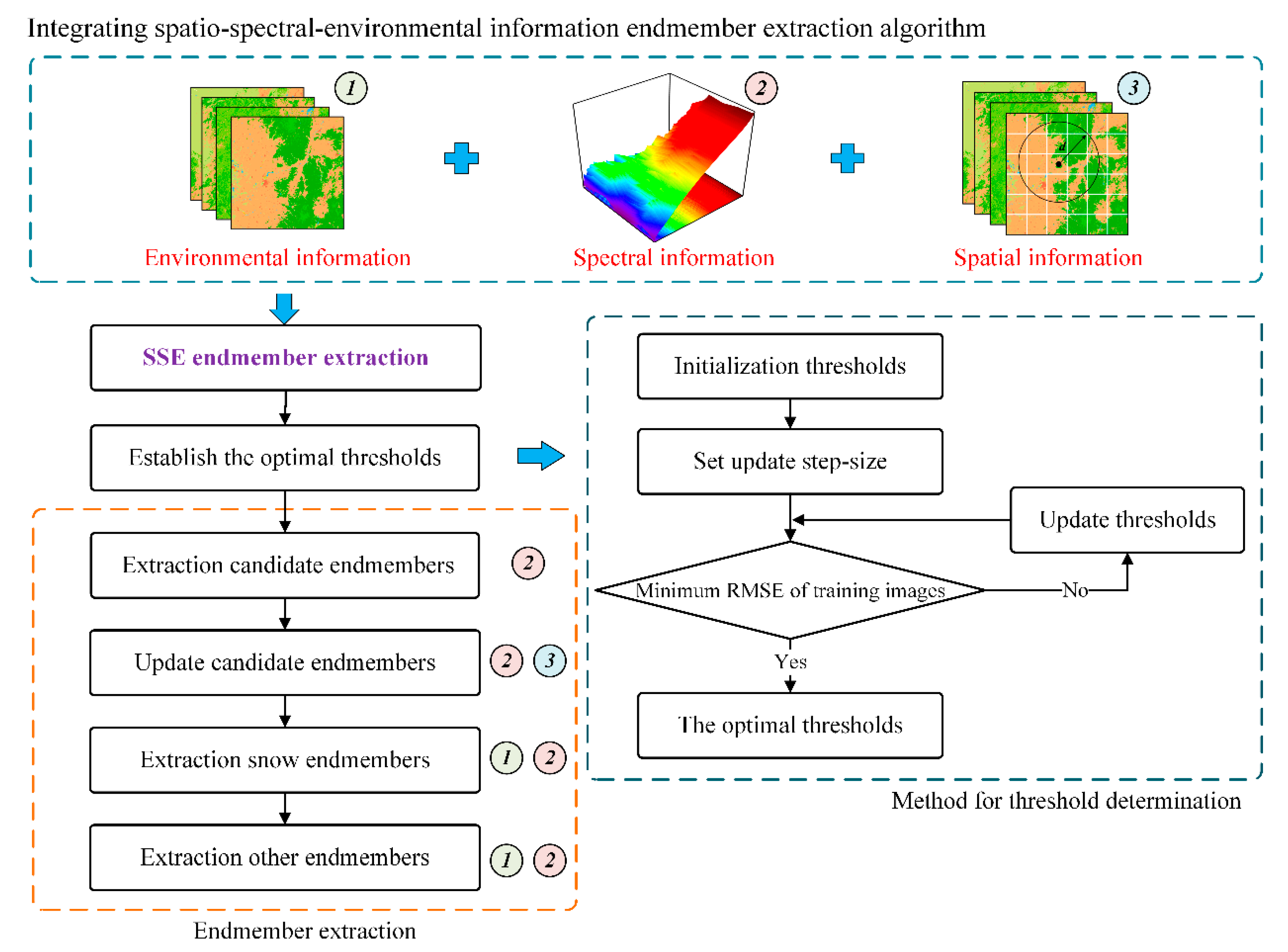The different materials have very small spectral discrepancies due to the influence of mixed pixels, making it difficult to accurately extract endmembers from images [39,40]. Furthermore, the same surface feature has different spectral curves on different images, whereas, the various surface objects have similar spectral curves on different images. Although different land-surface objects have very similar spectral information, their environmental information is very different, so the environmental information can be used as the prior knowledge of endmember extraction to initially determine the number of endmembers extracted from the image. Automatic extraction of endmembers from various images can reduce uncertainty caused by the heterogenicity of environmental information on different images.

In this study, we developed a new endmember extraction algorithm based on integrating the spatial-spectral-environmental (SSE) information, which can automatically extract endmembers from images. Then, combining the LSMA model, the SSE endmember extraction algorithm was applied to the MODIS FSC retrieval of China. The reference FSC generated by Landsat 8 binary snow cover maps with 30 m spatial resolution were used to quantitatively evaluate the accuracy of SSEmod. Meanwhile, the accuracy of SSEmod was compared with MODImLAB and MODSCAG for FSC retrieval. MODImLAB and MODSCAG are currently the most reliable algorithms for MODIS FSC retrieval based on LSMA model. MOD10A1 uses the semi-empirical linear model to calculate the MODIS FSC.

2. Materials

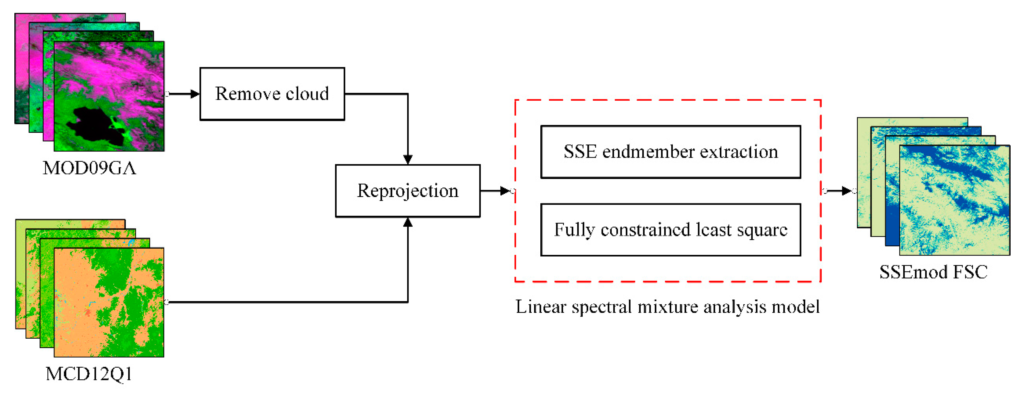
In this paper, we mainly utilize the MODIS surface reflectance product (MOD09GA Collection 6), Landsat 8 surface reflectance product, MODIS land cover product (MCD12Q1 Collection 6), and MODIS snow cover product (MOD10A1 Collection 6). MOD09GA is mainly used as the input data of SSEmod, MODImLAB, and MODSCAG. Landsat 8 mainly generates reference FSC. MCD12Q1, as vital environmental information, provides prior knowledge for the SSE endmember extraction algorithm.

2.1. MOD09GA

MOD09GA collection 6 was provided by NASA’s earth observing system data and information system (EOSDIS). MOD09GA daily products have accomplished atmospheric correction caused by the effects of atmospheric scattering and absorption [2].

MOD09GA images were selected according to Landsat 8 surface reflectance data with the same observation time and location, and re-projected with the same projection system as Landsat 8 images. Then, cloud cover pixels were removed through the quality assessment (QA) band of MODIS surface reflectance data. Finally, we implemented the SSE endmember extraction algorithm to extract endmembers of MOD09GA after removing cloud contamination.

2.2. Landsat 8 Surface Reflectance Data

Landsat 8 surface reflectance products are provided by the United States Geological Survey and have been completed atmospheric correction [41]. The Landsat 8 surface reflectance data were mainly used to produce reference FSC for validating the accuracy of SSEmod FSC.

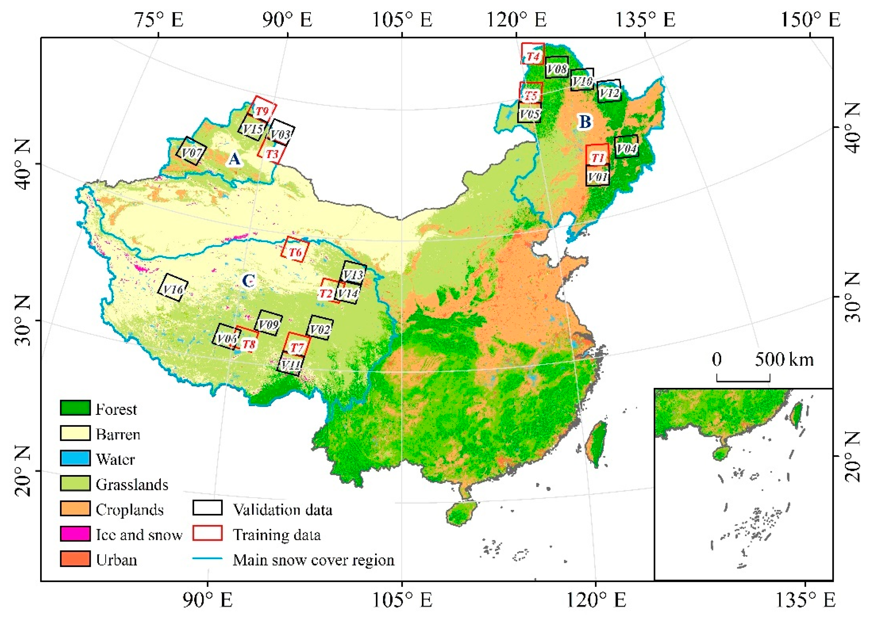
A total of 25 images were selected in three main snow cover regions of China (5 for northwestern China, 9 for northeastern China, and 11 for Qinghai–Tibet Plateau). The screening conditions were less than 1% in northwestern China and northeastern China, and less than 6% in the Qinghai–Tibet Plateau. Low cloud cover images are rare in the Qinghai–Tibet Plateau, which is affected by the high altitude of thin clouds and cirrus clouds. Screened images were divided into training datasets and validation datasets. Among them, 9 images were used to obtain the thresholds of the SSE endmembers extraction method, and 16 images were utilized to validate the accuracy of SSEmod FSC (Figure 1). Image pre-processing included: removal of cloud-contaminated pixels, terrain correction, and reference FSC retrieval. Firstly, the Quality Assessment (QA) band derived from the cloud and cloud shadow detection algorithm (CFMask) was used to remove cloud contaminative pixels from Landsat 8 surface reflectance images. C-correction is introduced to reduce the impact of topography on solar radiation, which is the most effective illumination correction for Landsat imagery [42]. We utilized different binary snow cover mapping methods for non-forest areas and forest areas. The SNOMAP algorithm, based on the spectral reflection characteristics of snow, has been widely used to produce standard MODIS global snow cover products. The NDSI is an integral part of the SNOMAP algorithm for the identification of snow. In addition, the NDSI-NDVI threshold field in SNOMAP can improve the accuracy of snow cover mapping in forest areas. Nevertheless, the forest-covered pixels were classified as snow-free conditions when the NDSI values were lower than 0.4, and NDVI values were lower than 0.3 [43]. In this paper, the SNOMAP algorithm is used to generate the reference Landsat 8 FSC in non-forest regions. In forest areas, the binary snow cover data is achieved by an improved algorithm for mapping snow cover through the normalized difference forest snow index [44]. The 30 m spatial resolution of binary snow cover images were re-sampled to 500 m spatial resolution of reference FSC using the multi-pixels aggregation method. All of the pre-processing processes have been accomplished with the Google Earth Engine [45].

2.3. MOD10A1

MOD10A1 Collection 6 is a widely used snow cover product globally. In C6, the FSC has been replaced by NDSI snow cover, generated through a series of screenings, such as surface temperature, low reflectance, cloud, and snow confusion, etc.

The pre-processing of MOD10A1 included image re-projection and FSC retrieval. MOD10A1 images were first re-projected with the same projection system as Landsat 8 surface reflectance. Then, the semi-empirical linear statistical relationship between FSC and NDSI was used to calculate MOD10A1 FSC. The empirical equation is given by:

$$\mathrm{FSC} = 1.45 \times \left(x/100\right)- 0.01$$

(1)

$x$ is the MOD10A1 NDSI snow cover. MOD10A1 FSC is mainly used to evaluate the accuracy of SSEmod FSC.

2.4. MCD12Q1

MCD12Q1 Version 6 products provide global land cover types at yearly intervals. The products have six different classification schemes and are derived using supervised classifications of MODIS Terra and Aqua reflectance data. The spatial resolution is 500 m, and the projection is a sinusoidal projection.

In this study, the International Geosphere-Biosphere Programme (IGBP) classification, as a very important environmental information, is used to distinguish forest and non-forest areas as well as to provide prior knowledge of endmember extraction. The number of endmembers extracted from images can roughly be estimated through major land cover types. IGBP codes from 1 to 9 were considered to represent forest-covered areas in which canopy height is more than 2 m and tree coverage is higher than 60%, whereas, other IGBP codes are classified as non-forest areas.

3. The SSE Endmember Extraction Method

This study developed a new endmember extraction algorithm combining spatial–spectral–environmental information to automatically extract endmembers from different images [46]. The main purpose of introducing land cover information is to initially estimate the number of endmembers and reduce the spectral redundancy of candidate endmembers. Additionally, different numbers and types of snow endmembers were extracted in forest areas and non-forest areas. Other endmembers were selected by the dynamic threshold segmentation method. The ultimate endmembers were adjusted through the spectral discrepancy of candidate endmember pixels. The SSE endmembers extraction algorithm consists of four steps: extraction candidate endmembers, update candidate endmembers, extraction snow endmembers, extraction other endmembers. A diagram of the SSE endmember extraction processing flow is presented in Figure 2.

3.1. Extraction Candidate Endmember

The entire image is divided into sub-regions of the same size. The optimal number of subregions $C$ can be calculated by:

$$C = \frac{\sqrt{mn}}{4}$$

(2)

m and n are columns and rows, respectively. Then, the PCA method is applied to calculate the eigenvalues and eigenvectors. The subregion data projected onto the extracted eigenvectors with the pixels that lie at either extreme of the vectors are retained, and these pixels represent the candidate endmembers set (Figure 3). The principal component analysis method radically enhances the spectral contrast and makes it easier to distinguish different materials with a small spectral discrepancy.

3.2. Update Candidate Endmembers

We introduced the thresholds $\omega$ and $\varpi$ to distinguish spectral similarity and update candidate endmember pixels (Figure 4). The SID-SAM method is adopted to measure spectral similarity [47]. The trial-and-error strategy is utilized to establish the optimal thresholds (in this study, $\omega$. is 0.1, $\varpi$. is 0.36). Let $Su{b}_i$ denote the i-th subregion, $U_i=\left\{s_1, s_2,s_k,\cdots ,s_n\right\}$ denote the candidate endmembers set of $Su{b}_i$, and n denote the total number of endmembers. Iterate each candidate endmember pixel in $U_i$ and use it as the central pixel of the $d\times d$ square sliding window, where $d$ is the Euclidean search distance (in this study, $d$ is 80). $s_k$ and $r_l=\left\{r_1, r_2,r_t,\cdots ,r_m\right\}$ denote central pixel and reference pixels set in the sliding window, where m is the total number of reference pixels. The rule of endmember update can be given by:

$$U_i^{*} = \{\begin{array}{cc}{U}_i + r_t& S\left(s_k,r_t\right)>\varpi ,r_t\in r_l, s_k\in U_i \\ U_i - s_k + \frac{s_k + {{\displaystyle \sum }}_{t=1}^{t=n}{r}_t}{n + 1}& S\left(s_k,r_t\right)<\omega ,r_t\in r_l, s_k\in U_i\end{array}$$

(3)

where $U_i^{*}$ is the updated candidate endmember set, $S\left(s_k,r_t\right)$ is the similarity of spectral vectors $s_k$ and $r_t$.

3.3. Extraction Snow Endmembers

We used land cover information to initially evaluate the numbers of endmembers that should be extracted from the image. Afterward, the spectral reference library was built with the reflectance of snow different underlying surfaces, grain sizes, and transformation periods measured by the Spectral Evolution’s PSR-3500 in the field is utilized to select the final snow endmembers from the candidate endmembers set. In this study, two snow endmembers and one snow endmember were extracted in forest areas and non-forest areas, respectively (Figure 5). Let $R=\left\{r{s}_1,r{s}_2,r{s}_3,\cdots ,r{s}_p\right\}$ denote the reference spectra of snow, and $U_v=\left\{s_v^1, s_v^2,s_v^3,\cdots ,s_v^m\right\}$ and $U_o=\left\{s_o^1, s_o^2,s_o^3,\cdots ,s_o^n\right\}$ denote the candidate endmembers set of the forest and non-forest areas. In forest areas, the first type of snow endmember $E_v^a$ and the second type of snow endmember $E_v^b$ can be obtained by Equations (4) and (5):

$$\begin{array}{cc}{E}_v^a=\frac{{{\displaystyle \sum }}_{k=1}^{k=l}{s}_v^k}{l}& U_v^{\prime }=\left\{s_v^k|s_v^k\in U_v \bigwedge \left(S\left(s_v^k, r{s}_j\right)<\frac{\omega }{2},r{s}_j\in R\right) \right\}\end{array}$$

(4)

$$\begin{array}{cc}{E}_v^b=\frac{{{\displaystyle \sum }}_{k=1}^{k=t}{s}_v^k}{t}& U_v^{″}=\left\{s_v^k|s_v^k\in \left(U_v-U^{\prime }\right) \bigwedge \left(S\left(s_v^k, r{s}_j\right)<\omega ,r{s}_j\in R\right) \right\}\end{array}$$

(5)

where $U_v^{\prime }$ and $U_v^{″}$ are the candidate endmember set that meets the constraint condition of Equations (4) and (5). In non-forest areas, the snow endmember $E_o^a$ can be calculated by Equation (6):

$$\begin{array}{cc}{E}_o^a=\frac{{{\displaystyle \sum }}_{k=1}^{k=e}{s}_o^k}{e}& U_o^{\prime }=\left\{s_o^k|s_o^k\in U_o \bigwedge \left(S\left(s_o^k, r{s}_j\right)<\omega ,r{s}_j\in R\right) \right\}\end{array}$$

(6)

where $U_o^{\prime }$ is the updated candidate endmember pixel set. $U_v^{″}$ and $U_o^{\prime }$ are utilized to extract other endmembers for forest and non-forest areas in the next step.

3.4. Extraction Other Endmembers

The dynamic threshold segmentation method is applied to extract other endmembers in the forest and non-forest areas (Figure 6). Let $n$ denote the number of endmembers finally extracted from the image (in this study, $4\le n\le 6$). $U_v^{″}$ and $U_o^{\prime }$ are update candidate endmember pixel sets in forest and non-forest areas, respectively. $E_v^i, i\in \left\{3, 4,\cdots ,6\right\}$, and $E_o^t, t\in \left\{2,3, \dots ,6\right\}$ denote other endmembers extracted in the different regions. $E_v^i$ and $E_o^t$ are given by Equations (7) and (8).

$$\begin{array}{cc}{E}_v^i = \frac{{{\displaystyle \sum }}_{j=1}^{j=l}{s}_v^k}{l}& U_v^i = \left\{s_v^k|s_v^k\in U_v^{i-1} \bigwedge \left(\delta <S\left(s_v^k, E_v^{i-1}\right)<S_{max}\right) \right\}\end{array}$$

(7)

$$\begin{array}{cc}{E}_o^t = \frac{{{\displaystyle \sum }}_{j=1}^{j=l}{s}_v^k}{l}& U_o^i = \left\{s_v^k|s_v^k\in U_o^{t-1} \bigwedge \left(\delta <S\left(s_o^k, E_o^{t-1}\right)<S_{max}\right) \right\}\end{array}$$

(8)

where $\delta = S_{max}-\left(S_{max}-S_{min}\right)/\left(n-1\right)$. $S_{max}$ and $S_{min}$ are the maximum and minimum spectral diversity between the updated candidate endmember set and the endmembers extracted in the previous iteration. $U_v^{i-1}$ and $U_o^{t-1}$ are updated candidate endmember sets from the previous iteration (for example, $U_v^{i-1}=U_v^{″}$ when extracting the third endmember set in forest areas). Repeat iteration for Equations (7) and (8) until $U_v^i=\varphi , U_o^i=\varphi$ or the number of extracted endmembers exceeds a predetermined value.

4. Application to MODIS Fractional Snow Cover Retrieval

The linear spectral mixture analysis model is a widely used approach to estimate the abundance of materials present in an image pixel [48,49,50]. The linear spectral mixture analysis model can be defined by

$$\mathit{R}=\mathit{E}\times \mathit{a}+\mathit{n}$$

(9)

where n accounts for the model error. $\mathit{R}$ is the reflectance vector located in (x, y) in MOD09GA. E is an endmembers matrix achieved by the SSE endmember extraction algorithm, and a is an abundance vector. Fully constrained least square is the state-of-the-art method to calculate the snow cover fractions for mixed pixels in the linear spectral mixture analysis model, which is comprised of the nonnegativity constrained least square and abundance sum-to-one constraint [51]. The estimate from the least-squares method is the one that minimizes the estimation residual. Finally, the fully constrained least square can be given by

$$\underset{\mathbf{\alpha }}{\min }\Vert \mathit{R}-\mathit{E}\mathbf{\alpha }{\Vert }_2^2$$

(10)

subject to

$$\{\begin{array}{c}\begin{array}{cc}0\le {\alpha }_i\le 1& i\in \left[1, m\right]\end{array}\\ {\displaystyle {\displaystyle \sum }_{i=1}^m}{\alpha }_i=1\end{array}$$

(11)

and m is the number of endmembers.

MOD09GA and land cover data feed into the spectral mixing analysis model. Adopt the SSE endmember extraction method to automatically extract MOD09GA endmembers. The fully constrained least square method is utilized to evaluate snow cover fractions on pixels level. In forest areas, the final FSC is the cumulative sum of snow cover fractions estimated by different snow endmembers in a pixel. The flowchart techniques for SSEmod FSC retrieval achieved through SSE endmember extraction and spectral mixture analysis model is shown in Figure 7.

5. Validation

MODImLAB and MODSCAG models were utilized to retrieve FSC in the main snow cover areas of China, respectively. We used a trial-and-error strategy to find the best numbers and types of endmembers with reliable performance for FSC retrieval at different times of the year. In addition, we adjusted the numbers and types of endmembers according to the land cover information in the study areas. Finally, three snow endmembers (medium granular snow, coarse granular snow, and transformed snow), dark vegetation, highlight vegetation, and soil, as the optimal endmembers, were used to retrieve FSC for MODImLAB and MODSCAG. The accuracy of the SSEmod FSC is evaluated with reference to Landsat 8 FSC. Simultaneously, we compared the accuracy of SSEmod FSC with MODSCAG FSC, MODImLAB FSC, and MOD10A1 FSC. The root-mean-square error (RMSE) and mean absolute error (MAE), as fractional metrics, were utilized to evaluate the accuracy of SSEmod FSC. Furthermore, we used a binary metric to assess the accuracy of SSEmod to eliminate total snow area influence on the fractional metric [52]. The precision estimates the probability that a pixel is correctly detected as snow.

$$precison=\frac{TP}{TP+FP}$$

(12)

where $TP$ (true positive) is the number of snow pixels of correct detection according to the reference, $FP$ (false positive) is the number of snow pixels that should be snow-free according to the reference. The recall is considered to evaluate the probability of a snow-covered pixel being detected.

$$recall=\frac{TP}{TP+FN}$$

(13)

where $FN$ (false negative) is the number of snow-free pixels that should be dictated as snow pixels according to the reference. $FScore$ evaluates the accuracy of snow detection without dependence on the total snow cover area.

$$FScore=\frac{2TP}{\left(2TP+FN+FP\right)}$$

(14)

For all of binary metrics, a pixel is considered as covered by snow if FSC > 0. To evaluate the accuracy of snow-covered areas evaluated by SSEmod FSC, the snow-covered area is compared with Landsat 8 FSC, MODSCAG FSC, MODImLAB FSC, and MOD10A1 FSC. Snow cover areas were calculated by:

$$SCA={\displaystyle \sum }_{i=1}^n{P}_i\ast {\left(s/1000\right)}^2$$

(15)

$P_i$ is FSC, $s$ is the spatial resolution of pixels, and $n$ is a total of pixels. We introduced the factor K, which is used to evaluate the model’s overestimating or underestimating snow cover area. $K=\left(SC{A}_a-SC{A}_b\right)/SC{A}_b$, where $SC{A}_a$ is the snow cover area of the estimated snow cover areas, and $SC{A}_b$ is snow cover area of Landsat 8 FSC.$\left|K\right|$ can reflect the biases of the estimated snow cover area.

5.1. Accuracy Assessment of SSEmod FSC in Different Snow-Covered Regions

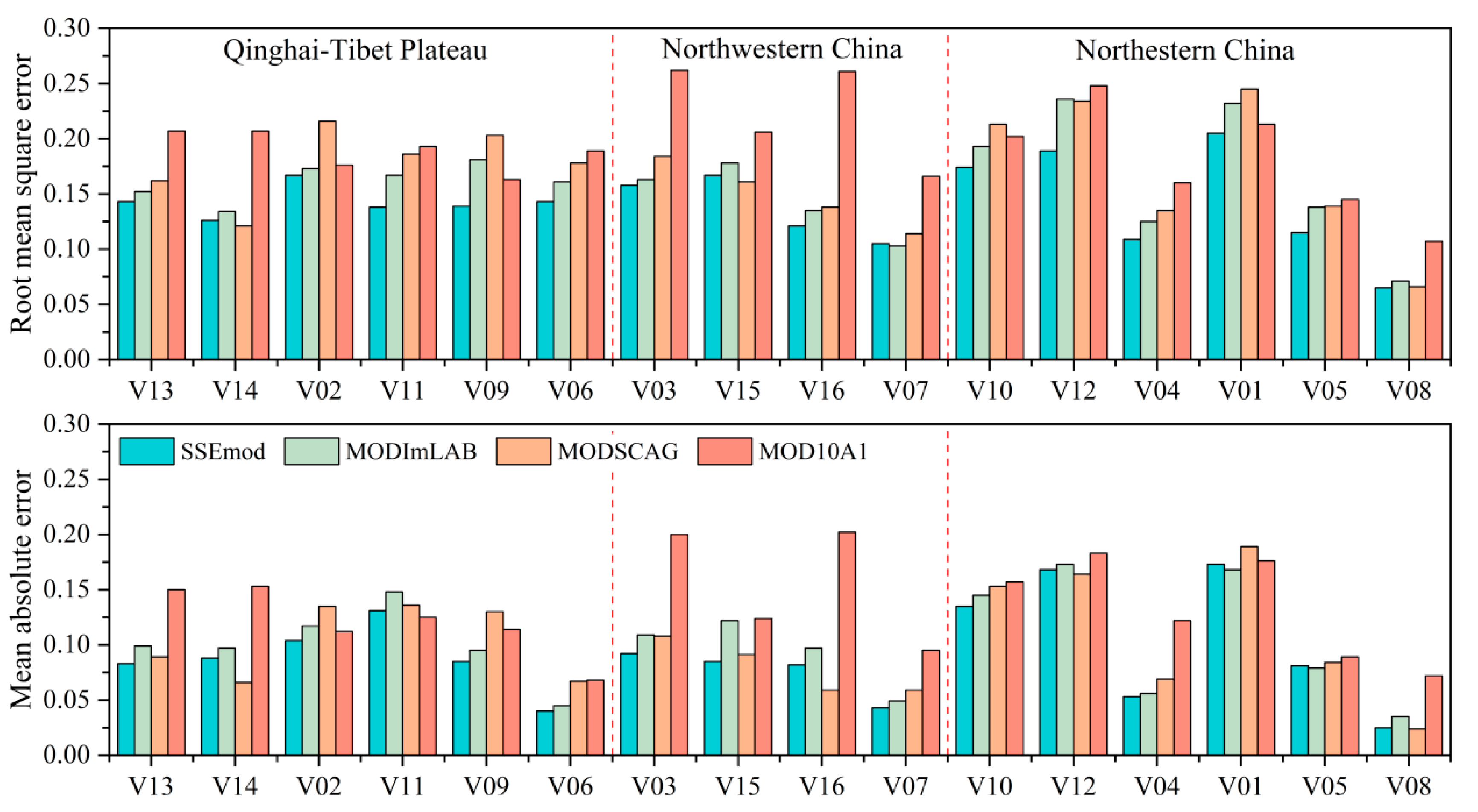
The validation results of the RMSE and MAE (fractional metrics) of the new endmembers extraction algorithm for FSC retrieval in different verification images in China’s main snow-covered areas are shown in Figure 8.

The validation results (Figure 8) show that the FSC retrieved by the linear spectral mixture analysis model is generally more accurate than the semi-empirical linear model. In all spectral mixing analysis models, we developed the new endmember extraction algorithm for FSC retrieval, which is more accurate than the other two most popular methods. The MODImLAB usually has higher accuracy than MODSCAG for FSC retrieval in different areas, although a few images have lower precision than MODSCAG. In addition, comparison of the accuracy of different snow cover regions, SSEmod FSC has poorer accuracy in northeastern China than that of northwestern China and the Qinghai–Tibet Plateau. We also calculated the average root-mean-square error (RMSE), mean absolute error (MAE), and binary metrics for different snow cover areas of China, simultaneously. The verification results are shown in

Table 1. The average accuracy validation results of different metrics of different methods for FSC retrieval in three snow-covered regions of China.

Regions.	Method	Precision	Recall	FScore	RMSE	MAE
Northeastern China	SSEmod	0.946	0.963	0.937	0.143	0.106
	MODImLAB	0.908	0.959	0.931	0.166	0.109
	MODSCAG	0.901	0.952	0.929	0.172	0.114
	MOD10A1	0.893	0.940	0.914	0.179	0.133
Qinghai–Tibet Plateau	SSEmod	0.934	0.810	0.846	0.138	0.089
	MODImLAB	0.904	0.788	0.807	0.161	0.100
	MODSCAG	0.895	0.731	0.802	0.164	0.104
	MOD10A1	0.873	0.718	0.782	0.174	0.117
Northwestern China	SSEmod	0.953	0.991	0.969	0.126	0.080
	MODImLAB	0.951	0.979	0.966	0.145	0.094
	MODSCAG	0.950	0.979	0.965	0.149	0.079
	MOD10A1	0.943	0.960	0.952	0.214	0.139

.

The results of all evaluated metrics show that our method can significantly improve FSC retrieval accuracy in different snow cover areas compared to other spectral mixture analysis models. In northeastern China, the SSEmod has the highest average precision, recall, and FScore. The average precision of SSEmod is 0.946, which indicates that our method has a small error for snow cover detection and that snow-free pixels are incorrectly classified as snow-covered pixels. The average recall score of MOD10A1 is the lowest compared to other models because many numbers of snow-covered pixels are not detected correctly. The average FScore of SSEmod is slightly higher than that of MODImLAB, which shows that SSEmod can more accurately identify the snow-covered or snow-free pixels. The average RMSE and MAE of SSEmod are also higher than those of other models. In the Qinghai–Tibet Plateau, the average precision of SSEmod is 0.934, which is higher than 0.904 for MODImLAB and 0.895 for MODSCAG. Meanwhile, the average recall and FScore of SSEmod are 0.810 and 0.864, both of which have significantly higher accuracy than other models. The RMSE and MAE of the semi-empirical linear model are 0.174 and 0.117, which behind the other three approaches based on the spectral mixture analysis model. In northwestern China, the ranking of the scores of evaluated metrics of all methods is very similar to the previous two snow cover regions, except for the recall metric score. We found that MODImLAB and MODSCAG have the same recall score. The MOD10A1 still has the lowest accuracy compared to other spectral mixing analysis models, and the average RMSE and MAE are 0.214 and 0.139, respectively, which are the highest compared to other regions.

Overall, the results show that using the spectral mixture analysis model to retrieve FSC is usually more accurate than that of the semi-empirical linear model. The MODImLAB method is slightly better than MODSCAG. As demonstrated by the FScore in all snow cover areas, all methods have the highest accuracy in northwestern China (0.969), followed by northeastern China (0.937), and the Qinghai–Tibet Plateau is the lowest (0.846). As shown by scores of all binary and fractional metrics, the SSEmod technique has the highest accuracy compared to the other methods, followed by MODImLAB, and the lowest is MOD10A1.

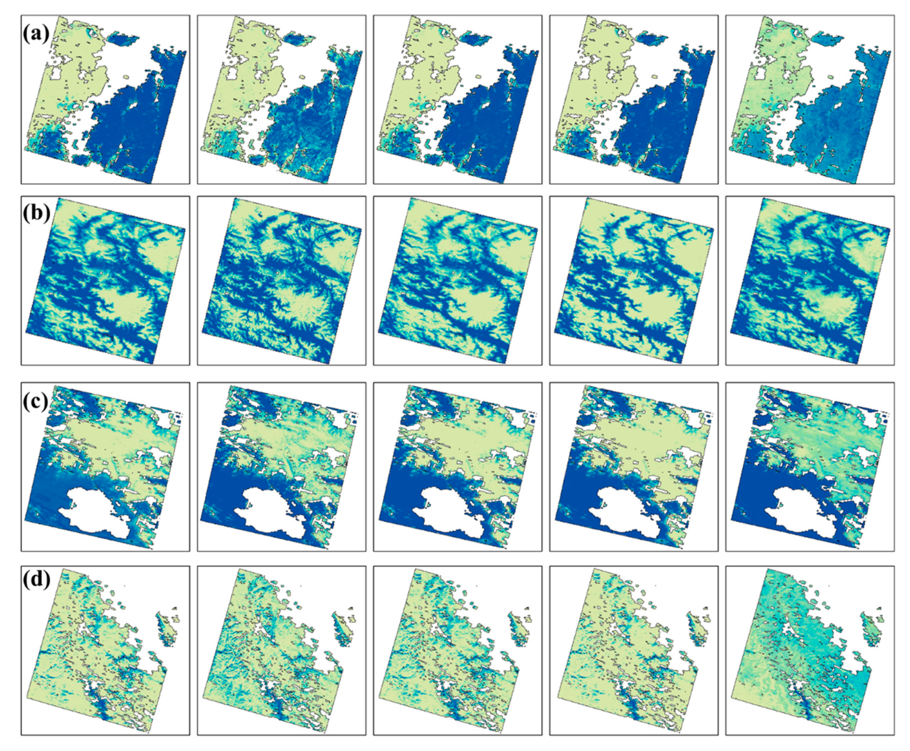
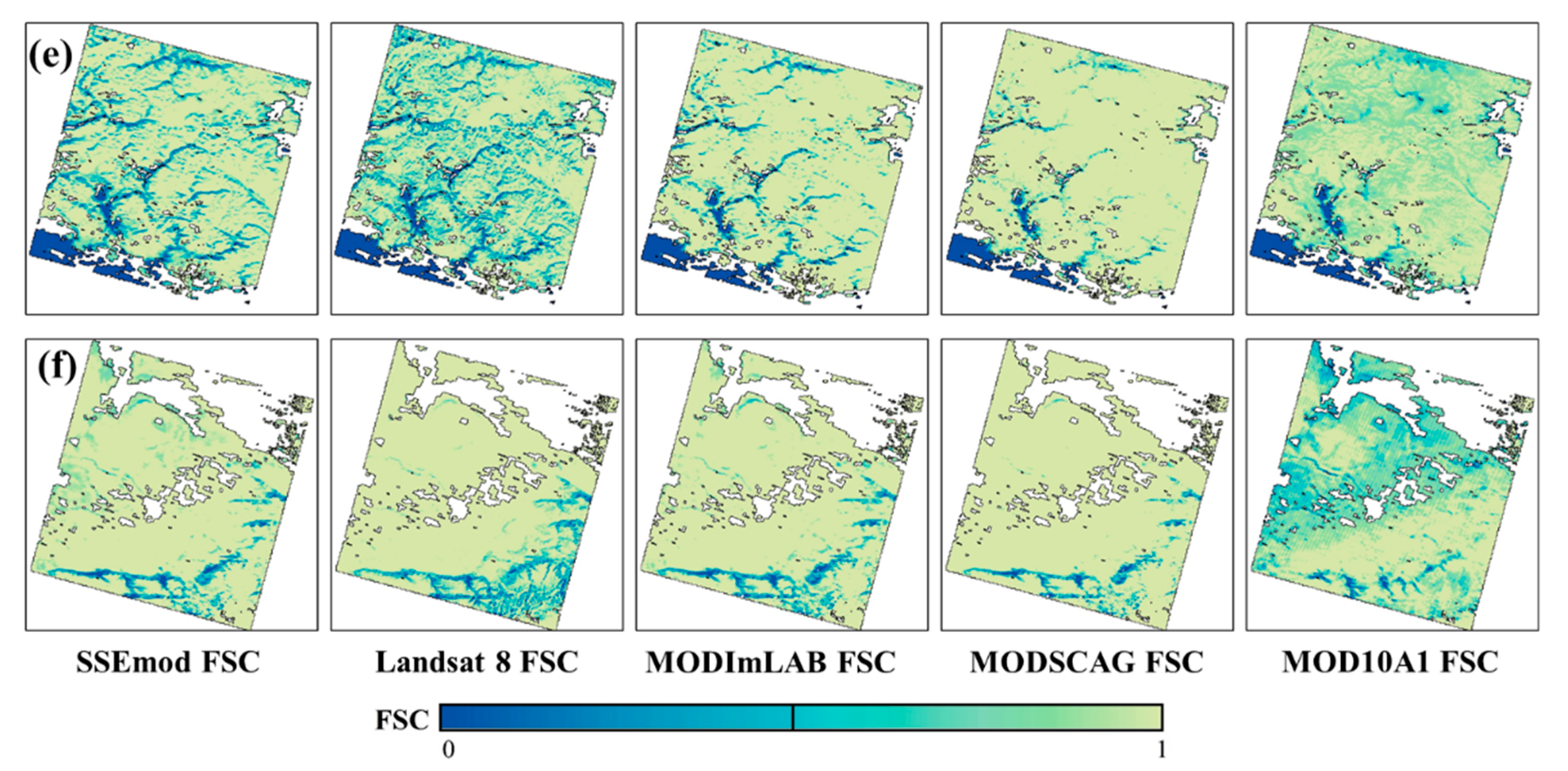
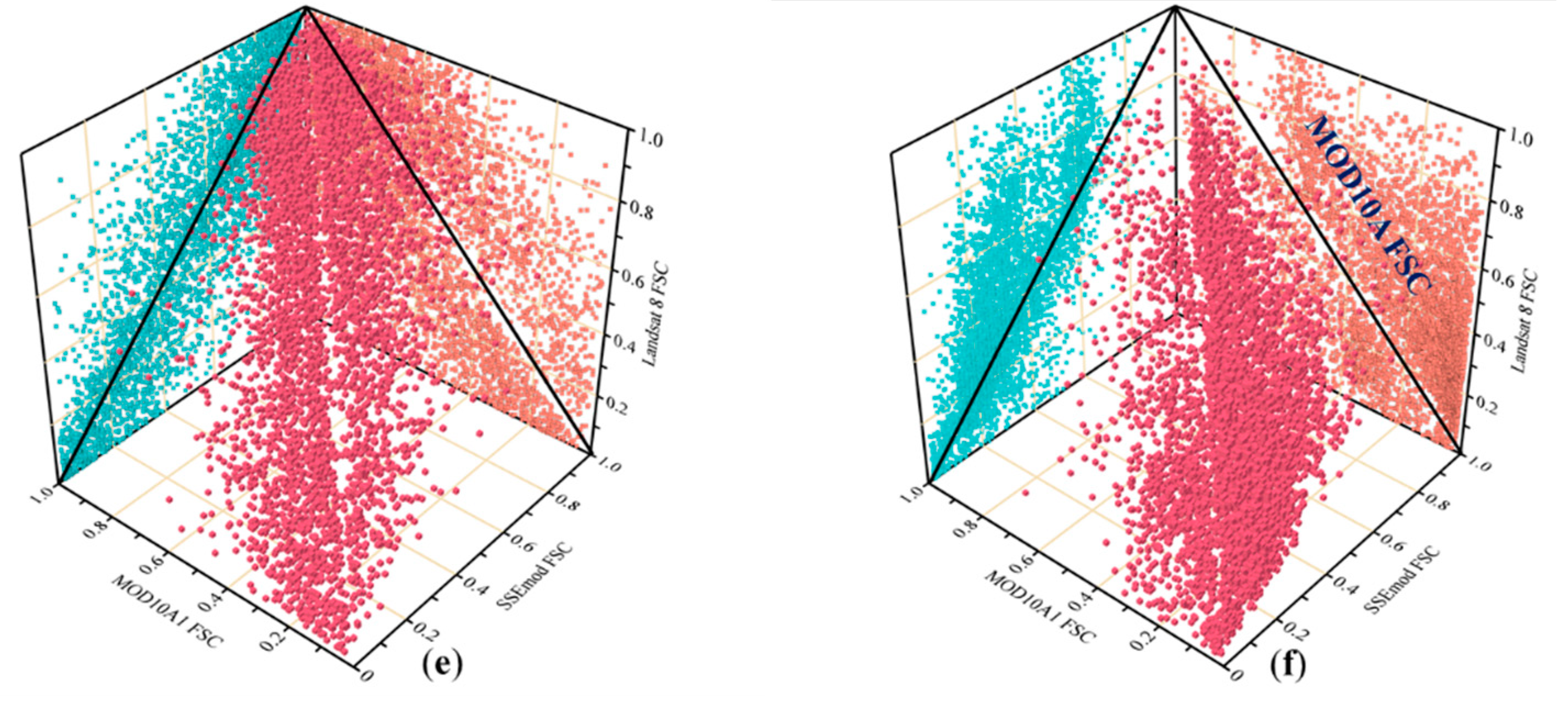
The results of FSC retrieval using the spectral mixture analysis models and the linear regression model are shown in Figure 9 (a selected from northeastern China, b and c selected from Qinghai–Tibet Plateau, d, e, and f selected from northwestern China). It can be clearly shown that all of the spectral mixture analysis models underestimate the snow-covered fraction in northeastern China, except for the linear regression model. However, the spectral mixture analysis model is better than the semi-empirical linear model in other snow cover areas.

5.2. Accuracy Assessment of SSEmod FSC in the Forest and Non-Forest Areas

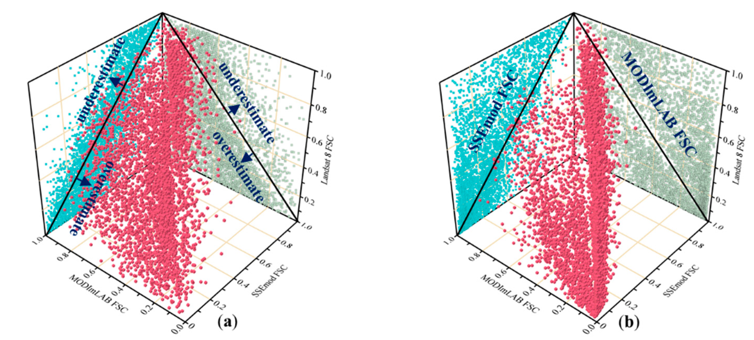
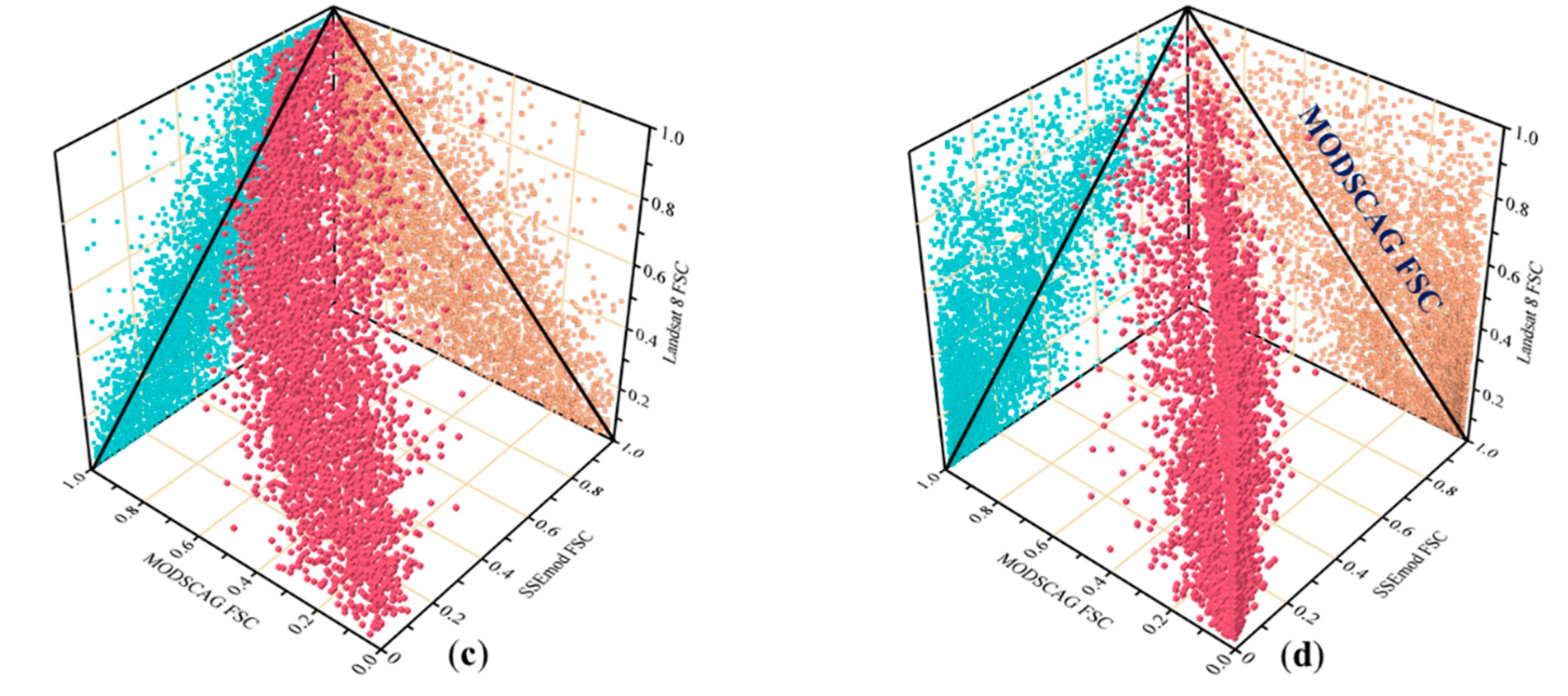
The accuracy validation result of FSC in the forest and non-forest regions are shown in Figure 10. The results of the validation of binary and fractional metrics are shown in

Table 2. The accuracy validation of binary and fractional metrics of FSC retrieved by the spectral mixture analysis models and semi-empirical linear model in forest areas and non-forest areas of the three main snow-covered regions of China.

Zone	Method	Precision	Recall	FScore	RMSE	MAE
Forest areas	SSEmod	0.941	0.668	0.828	0.165	0.119
	MODImLAB	0.934	0.631	0.756	0.196	0.125
	MODSCAG	0.930	0.617	0.742	0.201	0.127
	MOD10A1	0.863	0.591	0.701	0.216	0.132
Non-forest areas	SSEmod	0.962	0.982	0.952	0.107	0.065
	MODImLAB	0.928	0.975	0.946	0.126	0.092
	MODSCAG	0.921	0.977	0.948	0.129	0.093
	MOD10A1	0.903	0.948	0.945	0.162	0.128

.

In forest areas, the SSEmod has a precision score of 0.941, the highest compared to the other models, which shows that this method has a very small probability of identifying snow-free pixels as snow-covered pixels. The average score of recall of the SSEmod is 0.668, which better than other models. The 0.591 recall score of MOD10A1 is behind those of other spectral mixture analysis models because this method incorrectly detects many numbers of pixels that are actually covered by snow as snow-free pixels. The average FScore of SSEmod is 0.828, which is higher than other models and indicates that this method can more accurately evaluate the snow cover fraction. The average RMSE and MAE of SSEmod are 0.165 and 0.119, respectively. Compared to the different techniques for FSC retrieval, the SSEmod is more accurate in evaluating the snow cover fraction (Figure 10b,d,f). However, the spectral mixture analysis models and semi-empirical linear model underestimate the FSC due to the influence of trees in forest areas.

In non-forest areas, the precision ranking of different models is the same as the forest area. The average recall score of SSEmod is higher than other methods. Moreover, the average recall score of MODSCAG of 0.977 is better than the MODImLAB score of 0.975. The FScore of MODSCAG is slightly lower than that of MODSCAG. The RMSE and MAE of SSEmod are 0.107 and 0.065, respectively, which are significantly lower than those of the forest area (Figure 10a,c,e). As presented by the validation results of all evaluated metrics, whether of spectral mixture analysis models or semi-empirical linear model, the accuracy of FSC retrieval in non-forest areas is higher than that in forest areas.

In summary, the SSEmod has reliable accuracy in all regions, especially in non-forest areas. However, as shown in the recall score of Table 2, all of the FSC retrieval methods usually underestimate the snow cover fraction on the pixel level in forest areas. According to the precision and recall, it is challenging to find a universal approach to improve the accuracy of FSC retrieval in forest areas and non-forest areas. Compared to the RMSE of MODImLAB and MODSCAG, the accuracy of SSEmod is improved by 3.1% and 3.6% in forest areas, respectively, and in non-forest areas, it improved by 1.9% and 2.2%.

5.3. Accuracy Assessment of SSEmod FSC for Evaluation of Snow Cover Areas

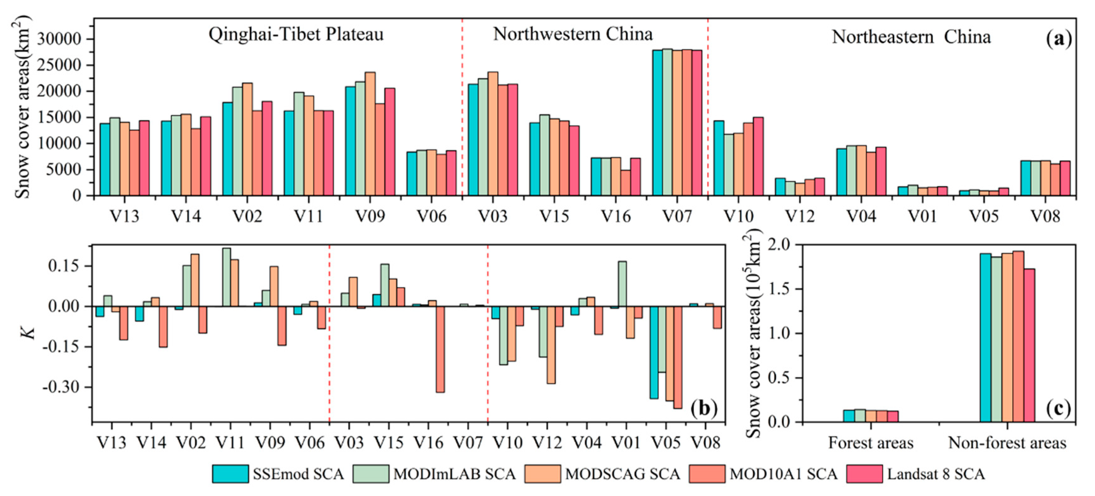
Figure 11a shows the accuracy validation results of the snow cover area (SCA) calculated with FSC that was retrieved by the different models in three snow cover regions of China. Figure 11b demonstrates the K value for various validation images. Figure 11c presents the accuracy validation results of the snow cover area in the forest and non-forest areas.

Table 3. The average of the absolute value of K in different snow cover regions.

Zone	|K|
	SSEmod	MODImLAB	MODSCAG	MOD10A1
Northeastern China	0.074	0.095	0.102	0.125
Qinghai–Tibet Plateau	0.026	0.062	0.068	0.094
Northwestern China	0.016	0.085	0.089	0.105
Average	0.039	0.081	0.086	0.108

shows the average of bias factor K of absolute value for evaluation of SCA in different snow cover regions, and

Table 4. The average of the absolute value of K in the forest and non-forest areas.

Zone	|K|
	SSEmod	MODImLAB	MODSCAG	MOD10A1
Forest areas	0.051	0.076	0.083	0.133
Non-forest areas	0.020	0.023	0.035	0.072
Average	0.036	0.050	0.059	0.103

shows the average of bias factor K of absolute value in the forest and non-forest areas.

K value and absolute K value represent the bias of applying FSC to estimate SCA. The negative K value indicates an underestimation of SCA, and vice versa. Although the SSEmod FSC has a very small estimation bias for 0.074, many validation images significantly underestimate the snow cover areas in northeastern China. In the Qinghai–Tibet Plateau and northwestern China, the bias of using the SSEmod FSC to estimate the SCA is 0.16 and 0.26, respectively, and which is better than that of other FSC estimates. The MODImLAB FSC and MODSCAG FSC have very similar accuracy for SCA estimation in different snow cover regions. In forest areas, the SSEmod FSC has an optimal estimation bias of 0.051 compared to the MODImLAB bias of 0.076. In non-forest areas, the estimation bias of SSEmod FSC is 0.020, which is very close to the estimation bias of MODImLAB of 0.023.

The result shows that SSEmod can more accurately estimate the SCA compared to other methods. The reliability of employing the MODImLAB to evaluate SCA is very similar to MODSCAG. The ability of SCA evaluation with FSC obtained by different approaches is consistent with the ranking of accuracy evaluated by binary and fractional metrics, which shows that the accuracy of SCA estimation is closely related to the FSC.

6. Discussion

6.1. The Error Source of FSC Retrieval

The surface temperature, environmental information (underlying surface information, topography, etc.), and atmospheric condition are vital factors that affect snow detection or FSC retrieval [53]. In the Qinghai–Tibet Plateau, the recall score is significantly lower than that of the other three regions, mainly due to the following reasons: many snow-covered pixels cannot correctly detect or be contaminated by the cloud. The reflectance of high-altitude cirrus clouds that include ice crystal is exactly similar to the pure snow reflectance, which easily causes cloud pixels’ contamination when extracting the endmembers. Although cloud mask can eliminate snow cover detection errors caused by the contamination of the cloud, it cannot completely remove cloud pixels from images due to errors of the cloud pixels’ identification algorithm. The surface temperature varies significantly in different regions due to its altitude differences. The solar radiation energy directly determines the different rates of snow-melting. Most forest resources are located in northeastern China. Coniferous forests are the primary land cover types in this area. Although the spectral mixture analysis methods have achieved excellent accuracy compared to the linear regression model, all of the techniques will also slightly underestimate the snow cover fraction. Two main factors cause the error in FSC retrieval in this area. One is that the algorithm of FSC retrieval should be improved one more time in forest areas, including the SSEmod, MODImLAB, and MODSCAG. The other is that a lot of dark pixels generate after atmospheric correction in the MOD09GA. In the clear sky, the tree canopy blocks the solar radiation reflected on the ground, which causes the satellite sensor to receive very low energy from the earth’s surface. Respectively, the dark pixels that have low reflectance values are mainly present in areas covered by dense vegetation. In the snow season, the dark pixels are usually covered with snow, but it is too difficult for all models to accurately estimate the snow cover fraction in forest areas, as shown in Table 1 and Table 2. In northwestern China, the land cover types are mainly non-forest land, which are grassland and cultivated land. Besides, the score of binary metrics is also higher than that of other regions, which indicates that the spectral mixture analysis model has a very small underestimation or overestimation error for snow detection. The local solar illumination and snow conditions are the main influence factors for the accuracy of FSC retrieval.

A systematic error is introduced into the reference FSC. The higher resolution images are used to produce binary snow cover data, and the multi-pixel aggregation technique is adopted to generate the reference FSC. The binary snow cover mapping method is used to detect the snow-covered pixels in non-forest areas and forest areas. Although the binary snow mapping method has reliable accuracy in non-forest areas and identifies snow pixels with snow cover fractions above 60%, it is problematic that only NDSI or NDFSI is employed to identify a thin-patch of snow cover for images [7,13]. The improved method based on multi-index and multi-threshold will also slightly underestimate the snow cover fractions in forest areas affected by trees, especially in dense vegetation-covered regions [13,43]. Besides, the SNOMAP method may not correctly detect the pixel that is actually covered by snow as a snow-covered pixel when the snow cover faction of a pixel is less than 60% [10]. At present, accurate identification of a thin patch of snow based on binary snow cover mapping is still a very challenging problem, which is mainly limited by the spatial resolution of the image and the algorithm for snow detection.

6.2. Comparison of Our Developed Method and Other Spectral Mixing Analysis Models

The new endmember extraction method for FSC retrieval can more accurately estimate snow cover fractions in pixel levels than other different approaches, as shown in the binary and fractional metrics score validation results. The fractional metrics are better than the binary metrics because the accuracy of the latter depends on the predetermined threshold for identifying as snow-covered or snow-free pixels.

The accuracy of diverse methods has a very significant discrepancy in different snow cover areas and underlying surfaces. Compared with other spectral mixture analysis models, the SSEmod has higher accuracy for estimating snow cover fraction. In northeastern China, the accuracy of SSEmod is improved by 2.3% and 2.9% compared to that of MODImLAB and MODSCAG (RMSE), respectively. In northwestern China, the accuracy of MODImLAB and MODSCAG are very close to SSEmod, and they are improved by 1.9% and 2.3%. In the Qinghai–Tibet Plateau, the accuracy of MODImLAB and MODSCAG are behind SSEmod by 2.3% and 2.6%. MODImLAB and MODSCAG have lower recall scores than SSEmod in forest areas, demonstrating that our method can detect snow-covered pixels more accurately. Likewise, the accuracy of SSEmod is also higher than MODImLAB and MODSCAG in non-forest areas, which are improved by 1.9% and 2.2% compared to other approaches.

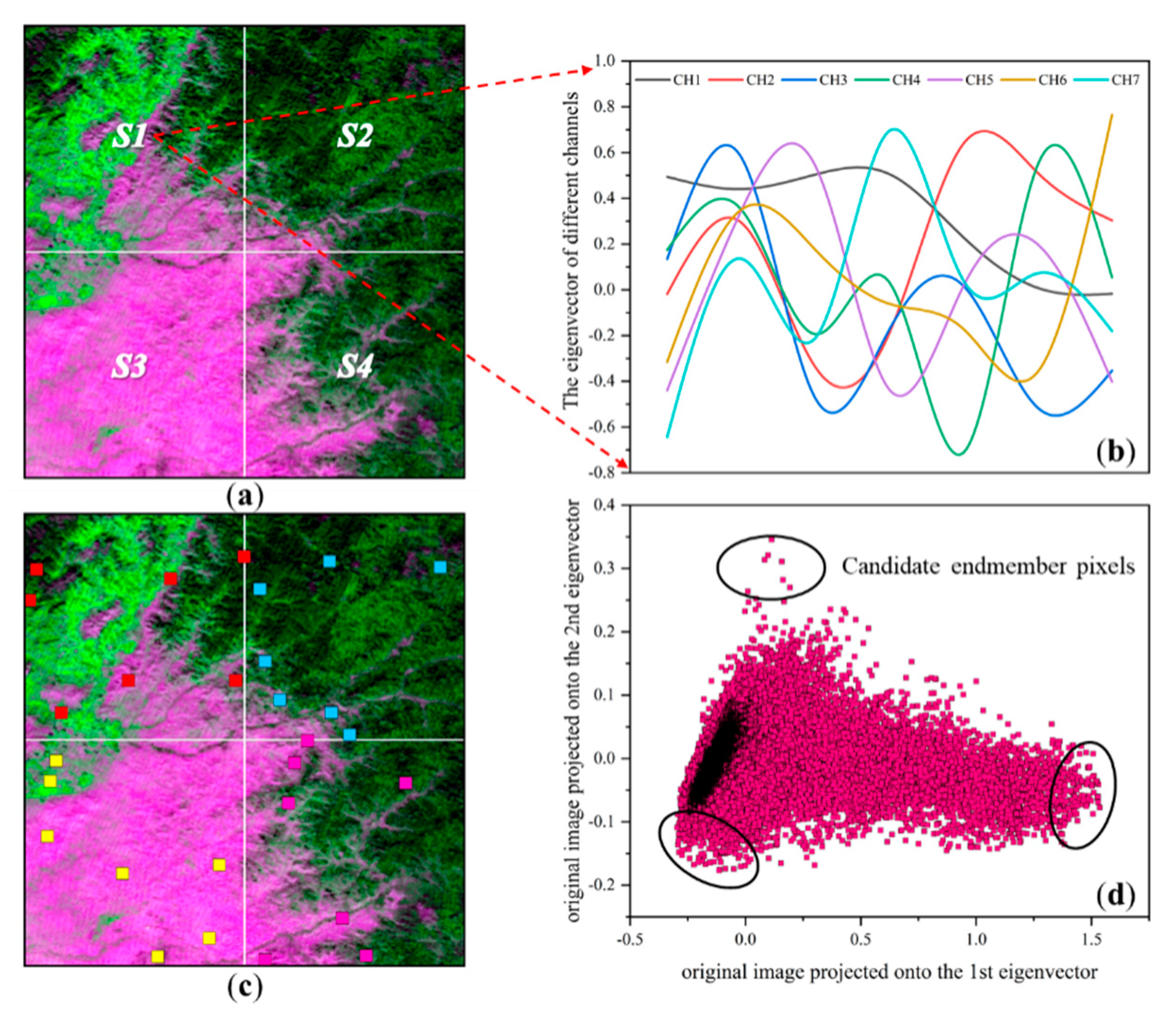
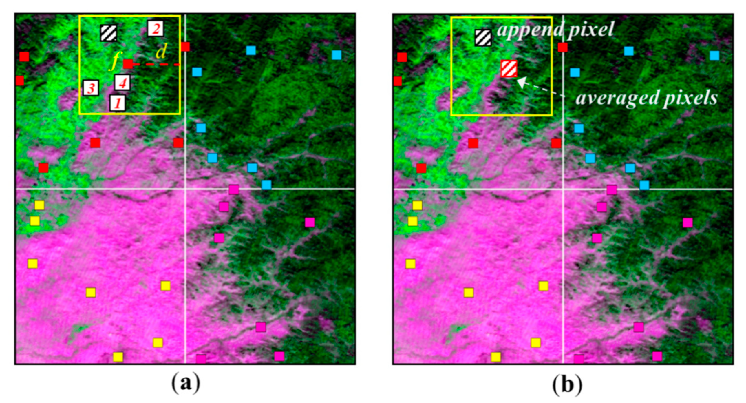
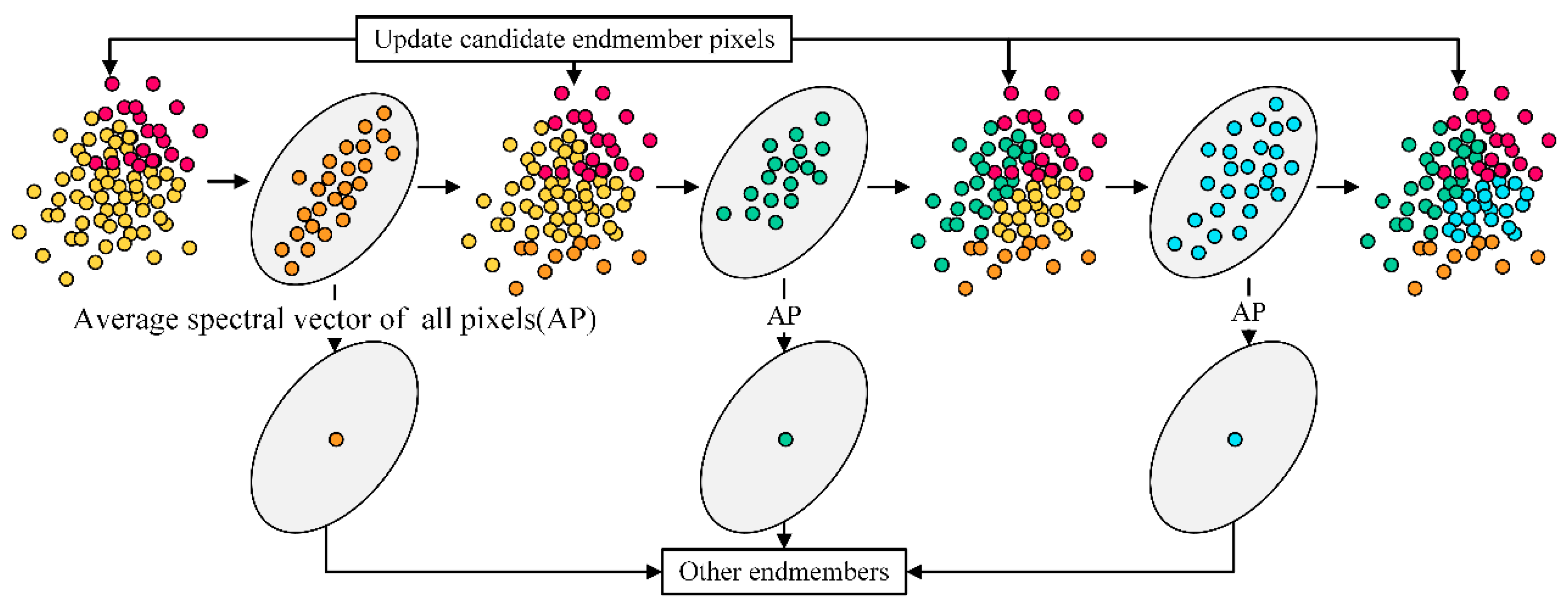
The method of endmember extraction directly affects the accuracy of snow cover fractions estimation in pixels level. The SSE endmember extraction algorithm can automatically extract endmembers from the image. It has an excellent advantage in that it can automatically determine the numbers and types of endmembers based on the spectral discrepancy of the candidate endmembers’ pixels. Nevertheless, MODImLAB and MODSCAG have fixed numbers and types of endmembers that cannot automatically extract from the image. MODSCAG also needs to consume a lot of computing resources. The snow endmembers of MODSCAG use the libraries of snow reflectance of different snow particle size calculated by the radiative transfer model. Other endmembers select from the spectral reference library of materials measured in the ground [19]. The MODImLAB finds the best set of endmembers that would be more robust to estimate the snow cover fraction from candidate endmembers directly chosen from the image using the trial-and-error strategy [20]. In reality, the best endmember extraction method should be able to extract different numbers and types of endmembers for diverse images, which can effectively reduce the error of endmember selection caused by the spectral discrepancy due to the season and solar radiation intensity influence in the same area. Especially in different seasons, the spectral contrast is the most significant. The average RMSE of all of the regions shows that the accuracy of MODSCAG (0.157) and MODImLAB (0.162) is behind to SSEmod (0.136). Overall, the SSE endmember extraction algorithm for snow cover fraction estimation can obtain reliable accuracy.

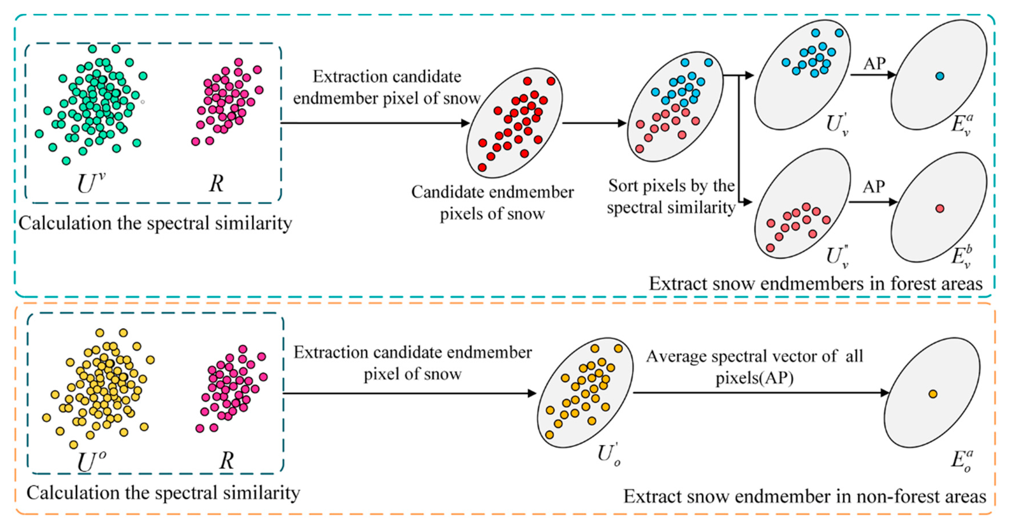
6.3. Why Extraction Two Different Types of Snow Endmembers in Forest Areas

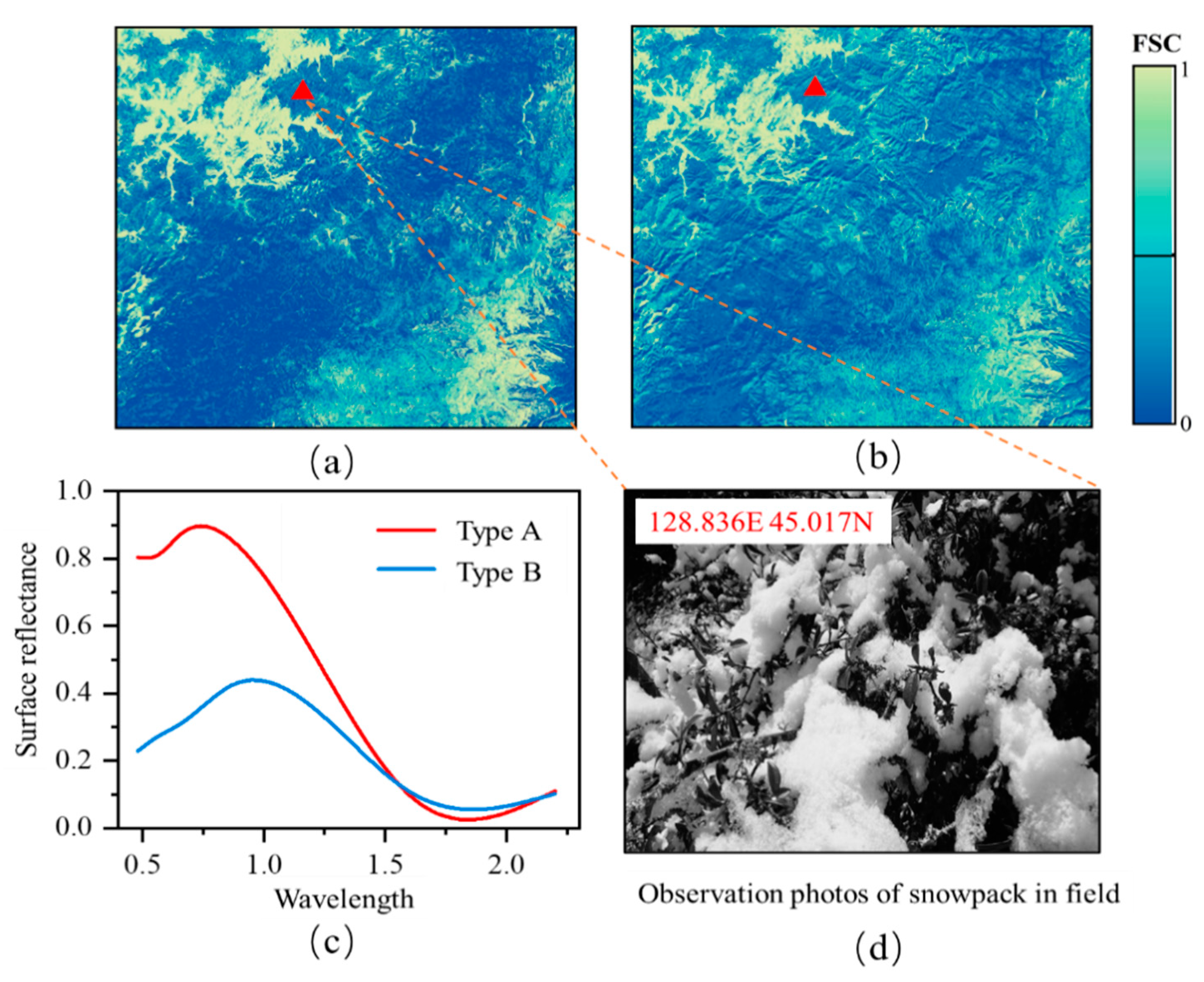
Extraction of different snow endmembers can more accurately estimate the snow cover fractions in forest areas (Figure 12). The snow endmembers should be pure snow reflectance at the pixel level. In fact, it is a great challenge to extract pure pixels from medium-resolution images due to the influence of vegetation, especially in dense vegetation-covered areas. We found that the snow reflectance of a pixel in dense vegetation-covered regions is hugely lower than that of sparsely forested areas. In addition, the snow cover fractions are most likely to be underestimated in dense vegetation-covered areas. The canopy region presents many dark pixels affected by the atmospheric correction for MODIS standard surface reflectance products. In sparse forest areas, the reflectance of snow-coved pixels is significantly higher than that of dense forest-covered areas. The error of estimation of snow cover fractions mainly comes from the influence of vegetation in this area. A trial-and-error strategy was used to find the optimal numbers of endmembers to a robust estimation of snow cover fractions for different images. When we extracted two snow endmembers, the mean error of all the training samples was ultimately the smallest in forest areas. One snow endmember was extracted from the area covered by dense vegetation, and the other was selected from the sparse vegetation-covered area.

6.4. Outlook of SSEmod

Compared with other spectral mixture analysis models for FSC retrieval, the SSE endmember extraction method achieves reliable accuracy in different snow cover regions. Our purpose is to develop an algorithm suitable for high accuracy FSC retrieval on a global scale. In future research, the SSEmod algorithm can still be improved in the following aspects:

The thresholds of spectral similarity assessment should be a series of dynamic values for different images. The SSE endmember extraction method introduces two different thresholds to evaluate the spectral similarity. We predetermine the optimal thresholds using the trial-and-error strategy to improve the execution efficiency of this algorithm, which can efficiently and robustly estimate the snow cover fractions of images at different time series and spatial locations. In reality, the spectral similarity of candidate endmembers varies with extra incident radiation energy observed by the satellite that is influenced by the solar intensity, solar zenith angle, atmospheric condition, and plant growth. Consequently, the best method is to select the optimal threshold according to different images.

More vital environmental information as prior knowledge should be absorbed into the endmember extraction algorithm or pre-processing. We consider the influence of underlying surface types on endmember extraction because the relationship between other environmental information and endmember extraction is very complicated, which will inevitably increase the time complexity of the algorithm. We are exploring this strategy, which absorbs the different environmental information, for example vegetation fraction, into the SSE endmember extraction algorithms to improve the accuracy of snow cover fraction estimation.

7. Conclusions

In this study, we developed a new method for the integration of spatial-spectral-environmental information to automatically extract endmembers from different images. Then, combined the linear spectral mixture analysis model to evaluate the snow cover fractions in different snow cover areas of China. Landsat 8 surface reflectance products were utilized to generate reference FSC to validate the accuracy of the SSEmod FSC. Simultaneously, we compared SSEmod FSC with MODImLAB, MODSCAG, and MOD10A1 FSC. The main conclusions are as follows:

The spectral analysis model can more accurately estimate the FSC compared to the semi-empirical linear model. The accuracy of the SSEmod, MODImLAB, and MODSCAG are significantly higher than the MOD10A1. For the average RMSE of all regions, the SSEmod is 0.136, which is improved by 2.1% and 2.6% compared to MODImLAB and MODSCAG, respectively. The SSEmod has a robust performance for FSC retrieval compared to MOD10A1. The RMSE of SSEmod is improved by 5.20% in all regions. The accuracy of all approaches has significantly improved in non-forest areas. SSEmod has the best performance for snow cover fraction estimation in northwestern China and has poor performance in northeastern China. Overall, the SSE endmember extraction method can more accurately evaluate the snow cover fraction in different snow cover areas of China.

Endmembers extraction from the medium-resolution image has a better advantage to estimate the snow cover fraction compared to endmembers extraction from spectral reference libraries built with the reflectance of materials measured in the field. In addition, the method of fixing the number and type of endmembers usually has lower precision than the method of not fixing it. The SSE algorithm can automatically extract different numbers and types of endmembers from diverse images.

Introducing environmental information into the endmember extraction can remarkably improve the accuracy of FSC retrieval. Land cover types, as crucial environmental information, are absorbed into the SSE endmember extraction algorithm, which can initially estimate the number of endmembers and effectively reduce the spectral redundancy of the candidate endmembers. Especially when the spectral contrast is very low, the land cover information can effectively distinguish different materials. The endmember extraction method, combined with multi-source information, can effectively utilize spatial and environmental information to increase the spectral diversity of the entire image so that endmembers can be extracted more easily from different images.

Extracting different types of snow endmembers can effectively improve the accuracy of FSC retrieval in forest-covered areas. The SSEmod method achieves a reliable accuracy for FSC retrieval in forest areas. The average RMSE of MODImLAB and MODSCAG is behind by 3.1% and 3.6% compared to SSEmod in forest areas. Compared with MOD10A1, the RMSE of SSEmod is improved by 5.1% in this area. All of the approaches slightly underestimate the snow cover fraction due to the influence of the trees and dark pixels in forest areas. In summary, the SSEmod has reliable accuracy for FSC retrieval compared to MODImLAB and MODSCAG in forest areas.