Forest Fire Susceptibility Prediction Based on Machine Learning Models with Resampling Algorithms on Remote Sensing Data

 ,
,  ,
,  and
and 
Abstract

1. Introduction
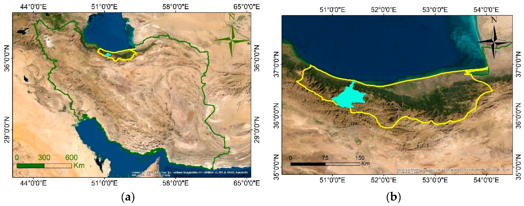
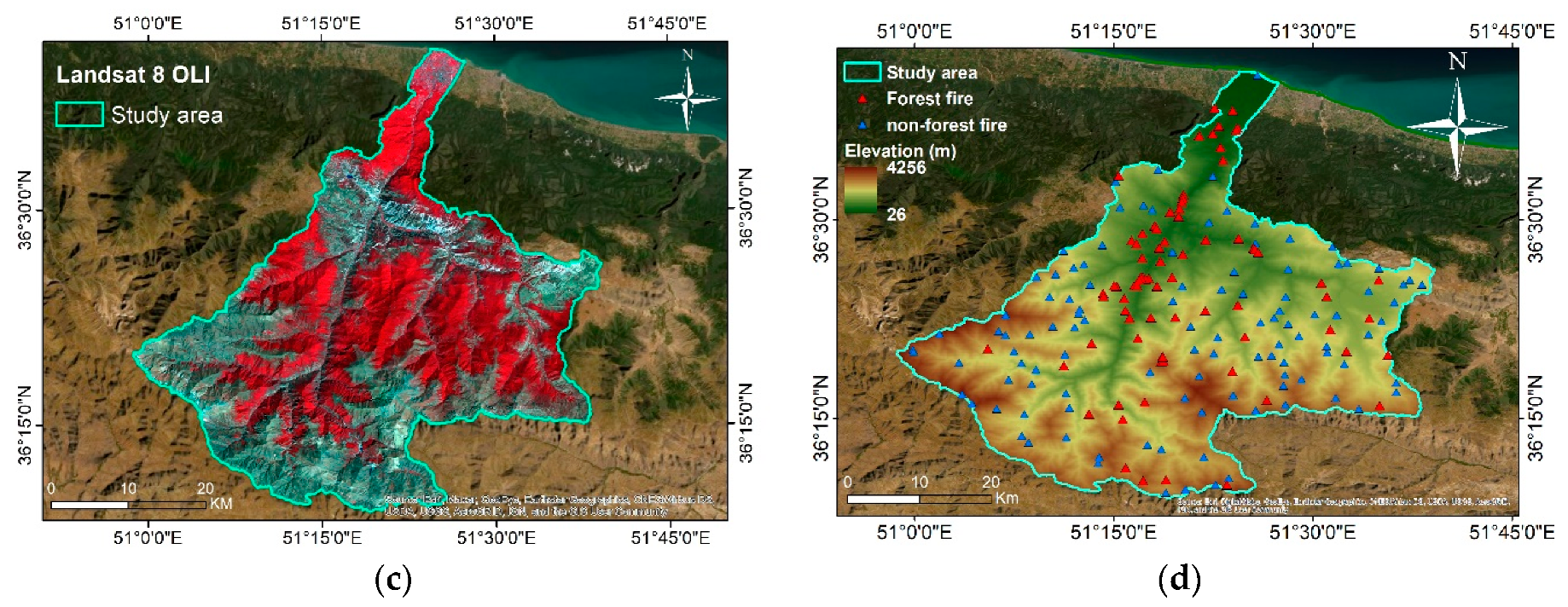
2. Study Area
3. Methodology
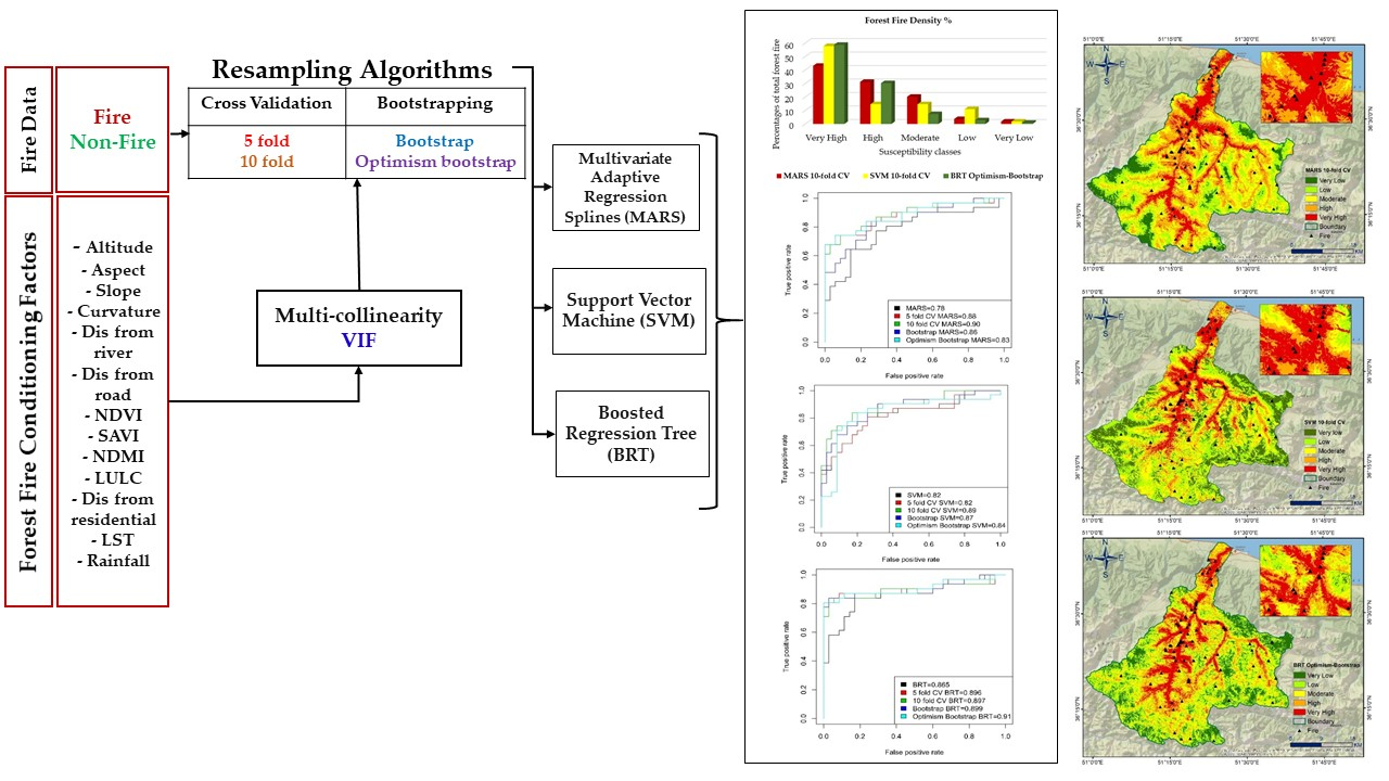
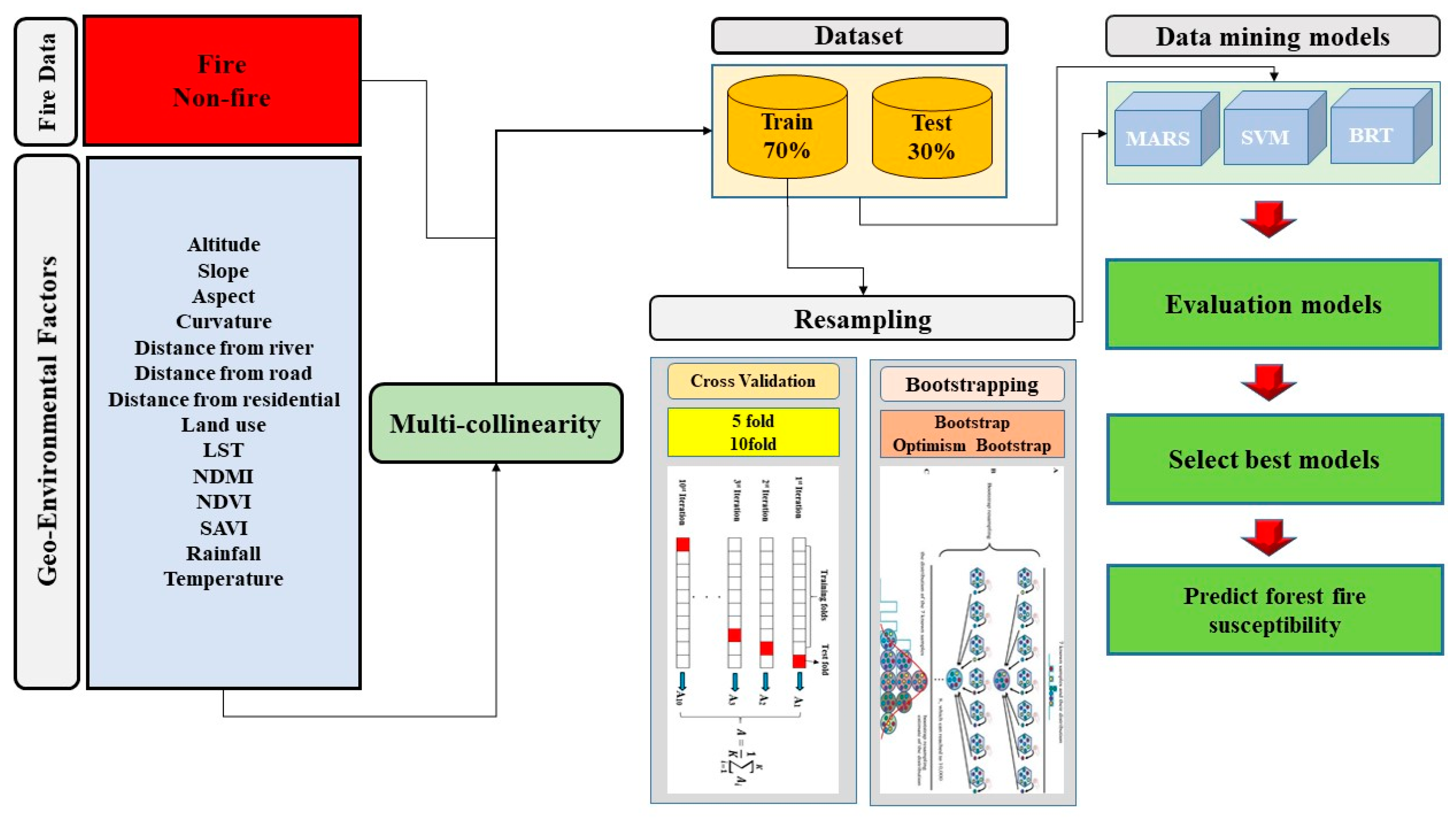
3.1. Overview
3.2. Data Preparation
3.3. Factor Analysis
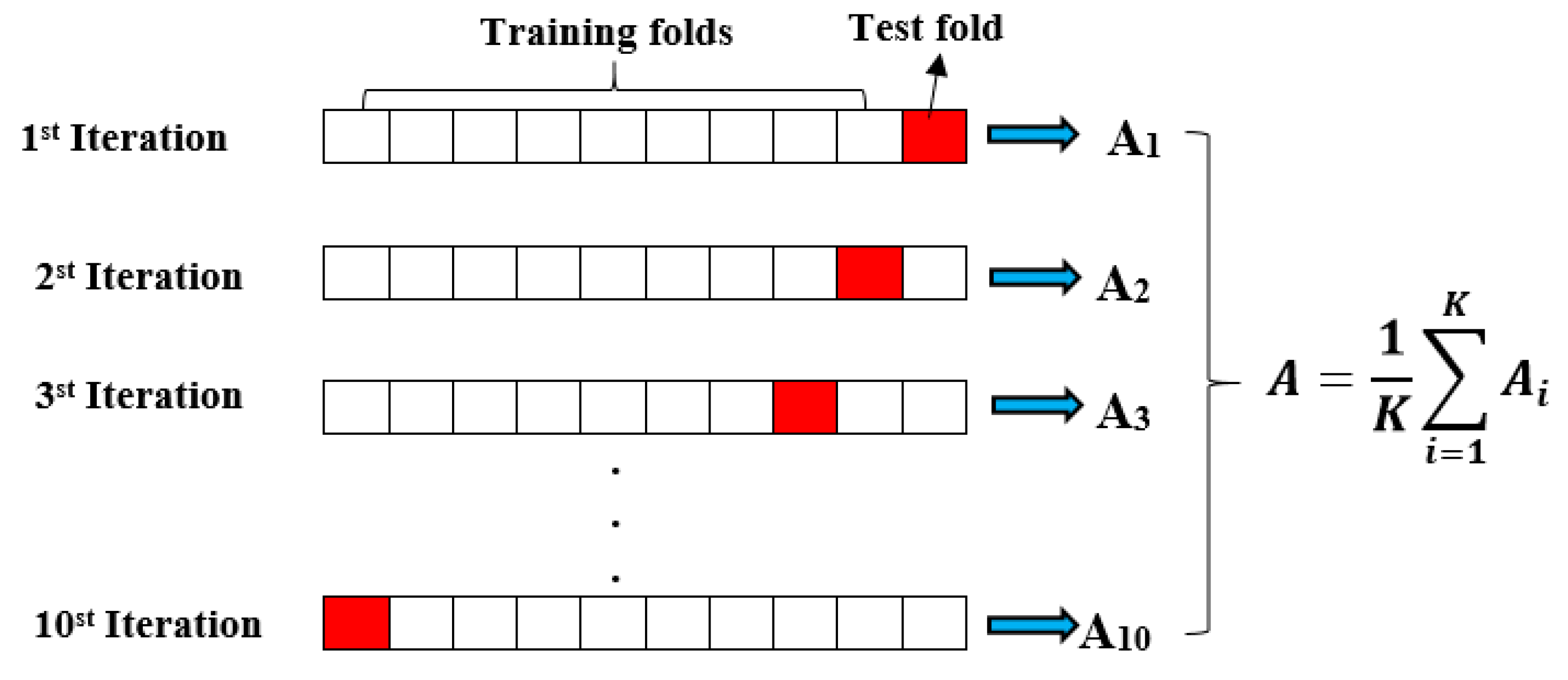
3.4. Resampling: Cross Validation (CV), Bootstrap and Optimism Bootstrap
3.5. Model Implementation
3.5.1. Multivariate Adaptive Regression Splines (MARS)
3.5.2. Support Vector Machine (SVM)
3.5.3. Boosted Regression Tree (BRT)
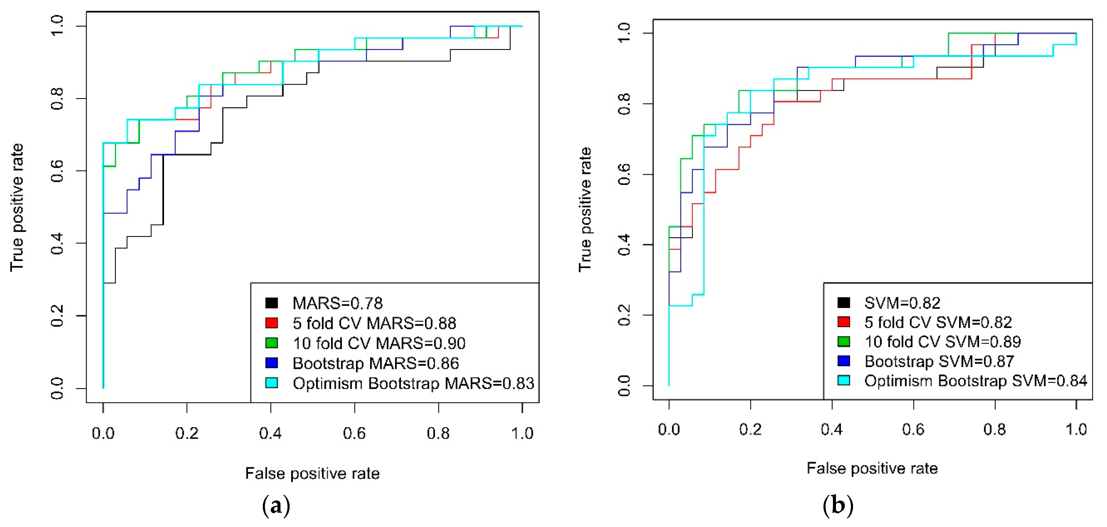
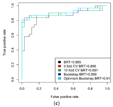
3.6. Validation
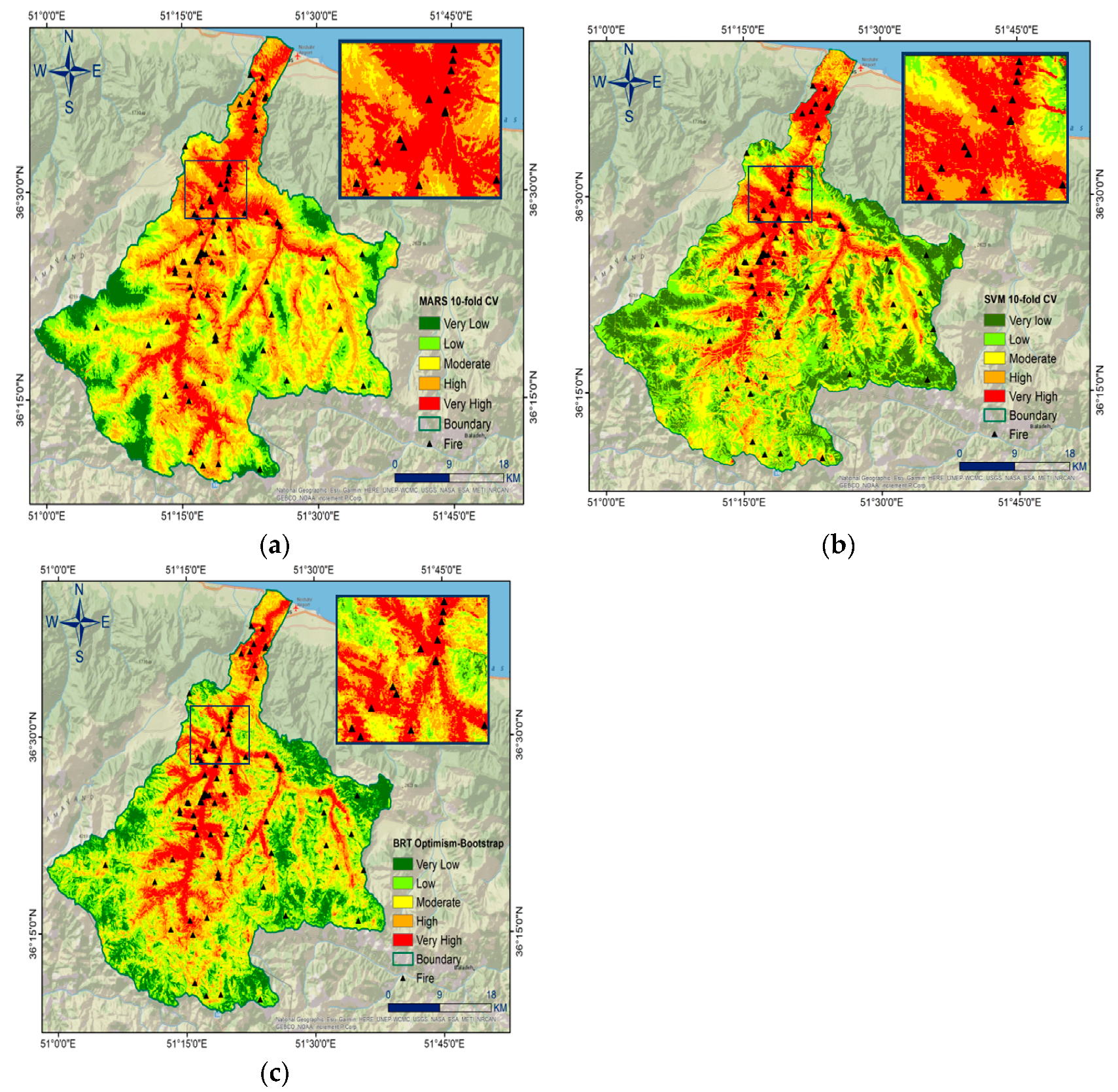
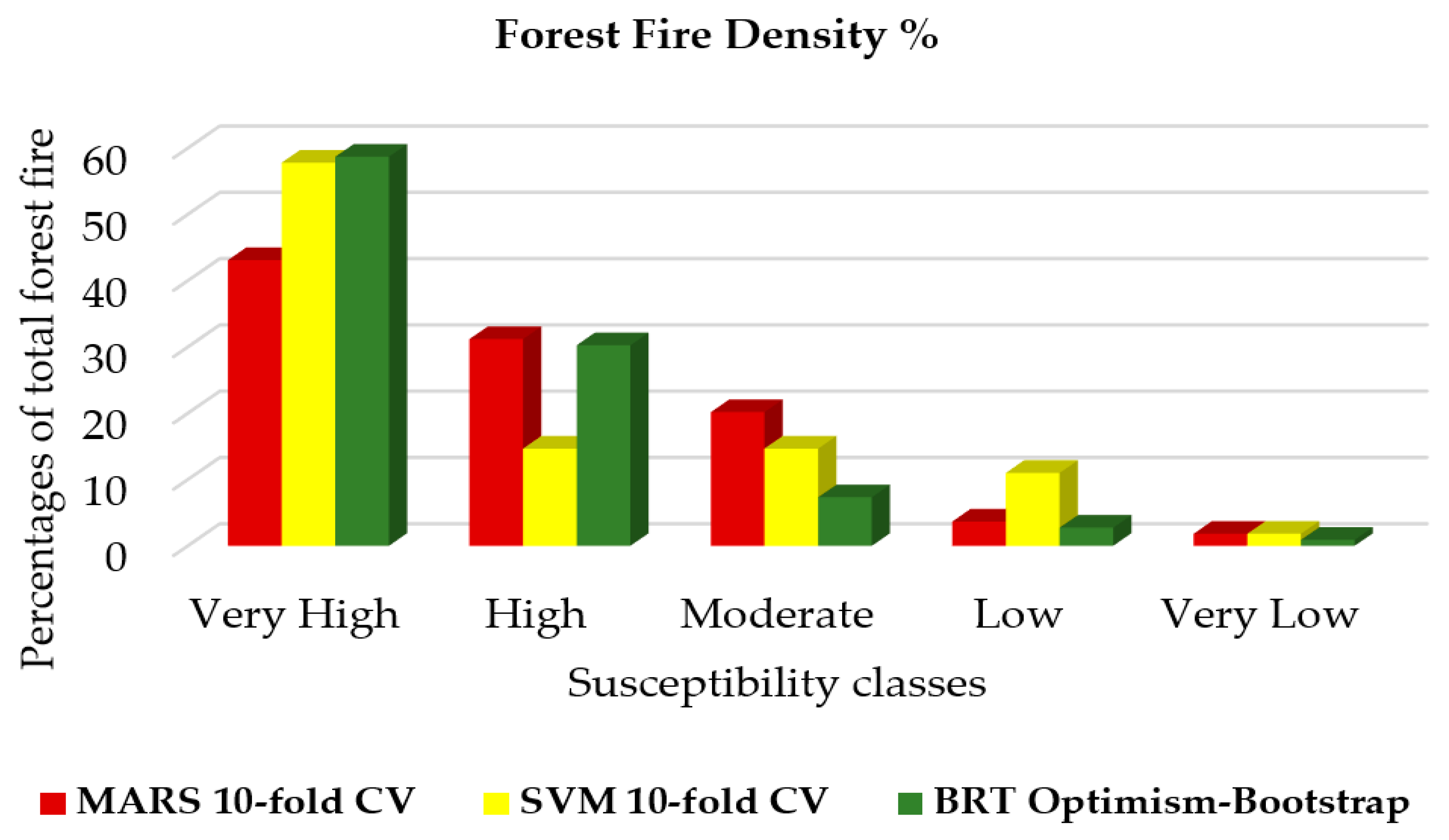
4. Results
5. Discussion
6. Conclusions
Author Contributions
Funding
Acknowledgments
Conflicts of Interest
References
- Bui, D.T.; Le, K.T.T.; Nguyen, V.C.; Le, H.D.; Revhaug, I. Tropical forest fire susceptibility mapping at the Cat Ba National Park area, Hai Phong City, Vietnam, using GIS-based Kernel logistic regression. Remote Sens. 2016, 8, 347. [Google Scholar] [CrossRef]
- Balch, J.K.; Bradley, B.A.; Abatzoglou, J.T.; Chelsea Nagy, R.; Fusco, E.J.; Mahood, A.L. Human-started wildfires expand the fire niche across the United States. Proc. Natl. Acad. Sci. USA 2017, 114, 2946–2951. [Google Scholar] [CrossRef] [PubMed]
- Randerson, J.T.; Liu, H.; Flanner, M.G.; Chambers, S.D.; Jin, Y.; Hess, P.G.; Pfister, G.; Mack, M.C.; Treseder, K.K.; Welp, L.R.; et al. The impact of boreal forest fire on climate warming. Science 2006, 314, 1130–1133. [Google Scholar] [CrossRef] [PubMed]
- Ireland, G.; Petropoulos, G.P. Exploring the relationships between post- fire vegetation regeneration dynamics, topography and burn severity: A case study from the Montane Cordillera Ecozones of Western Canada. Appl. Geogr. 2015, 56, 232–248. [Google Scholar] [CrossRef]
- Nölte, A.; Meilby, H.; Yousefpour, R. Multi-purpose forest management in the tropics: Incorporating values of carbon, biodiversity and timber in managing Tectona grandis (teak) plantations in Costa Rica. For. Ecol. Manag. 2018, 422, 345–357. [Google Scholar] [CrossRef]
- Lamb, D.; Erskine, P.D.; Parrotta, J.A. Restoration of degraded tropical forest landscapes. Science 2005, 310, 1628–1632. [Google Scholar] [CrossRef]
- Brown, A.R.; Petropoulos, G.P.; Ferentinos, K.P. Appraisal of the Sentinel-1 & 2 use in a large-scale wildfire assessment: A case study from Portugal’s fires of 2017. Appl. Geogr. 2018, 100, 78–89. [Google Scholar]
- Bruinsma, J. Towards sustainable forestry. In World Agriculture: Towards 2015/2030: An FAO Perspective; Diouf, J., Ed.; Earthscan Publications Ltd.: London, UK, 2003. [Google Scholar]
- Pricope, N.G.; Binford, M.W. A spatio-temporal analysis of fire recurrence and extent for semi-arid savanna ecosystems in southern Africa using moderate-resolution satellite imagery. J. Environ. Manag. 2012, 100, 72–85. [Google Scholar] [CrossRef]
- Key, C.H.; Benson, N.C. Landscape assessment: Remote sensing of severity, the normalized burn ratio and ground measure of severity, the composite burn index. In FIREMON: Fire Effects Monitoring and Inventory System; General Technical Report; RMRS-GTR-164-CD; LA1-LA51; U.S. Department of Agriculture, Forest Service, Rocky Mountain Research Station: Fort Collins, CO, USA, 2005; pp. 305–325. [Google Scholar]
- Ghorbanzadeh, O.; Valizadeh Kamran, K.; Blaschke, T.; Aryal, J.; Naboureh, A.; Einali, J.; Bian, J. Spatial Prediction of Wildfire Susceptibility Using Field Survey GPS Data and Machine Learning Approaches. Fire 2019, 2, 43. [Google Scholar] [CrossRef]
- Pourtaghi, Z.S.; Pourghasemi, H.R.; Aretano, R.; Semeraro, T. Investigation of general indicators influencing on forest fire and its susceptibility modeling using different data mining techniques. Ecol. Indic. 2016, 64, 72–84. [Google Scholar] [CrossRef]
- Tshering, K.; Thinley, P.; Shafapour Tehrany, M.; Thinley, U.; Shabani, F. A Comparison of the qualitative analytic hierarchy process and the quantitative frequency ratio techniques in predicting forest fire-prone areas in Bhutan using GIS. Forecasting 2020, 2, 36–58. [Google Scholar] [CrossRef]
- Syifa, M.; Panahi, M.; Lee, C.W. Mapping of post-wildfire burned area using a hybrid algorithm and satellite data: The case of the camp fire wildfire in California, USA. Remote Sens. 2020, 12, 623. [Google Scholar] [CrossRef]
- Lang, N.; Schindler, K.; Wegner, J.D. Country-wide high-resolution vegetation height mapping with Sentinel-2. Remote Sens. Environ. 2019, 233, 111347. [Google Scholar] [CrossRef]
- Roteta, E.; Bastarrika, A.; Padilla, M.; Storm, T.; Chuvieco, E. Development of a Sentinel-2 burned area algorithm: Generation of a small fi re database for sub-Saharan Africa. Remote Sens. Environ. 2019, 222, 1–17. [Google Scholar] [CrossRef]
- Navarro, G.; Caballero, I.; Silva, G.; Parra, P.C.; Vázquez, Á.; Caldeira, R. Evaluation of forest fire on Madeira Island using Sentinel-2A MSI imagery. Int. J. Appl. Earth Obs. Geoinf. 2017, 58, 97–106. [Google Scholar] [CrossRef]
- Jain, P.; Coogan, S.C.P.; Subramanian, S.G.; Crowley, M.; Taylor, S.; Flannigan, M.D. A review of machine learning applications in wildfire science and management. arXiv 2020, arXiv:2003.00646. [Google Scholar] [CrossRef]
- Liang, H.A.O.; Zhang, M.; Wang, H. A neural network model for wildfire scale prediction using meteorological factors. IEEE Access 2020, 7, 176746–176755. [Google Scholar] [CrossRef]
- Tien, D.; Bui, Q.; Nguyen, Q.; Pradhan, B. A hybrid artificial intelligence approach using GIS-based neural-fuzzy inference system and particle swarm optimization for forest fire susceptibility modeling at a tropical area. Agric. For. Meteorol. 2017, 233, 32–44. [Google Scholar] [CrossRef]
- Gigović, L.; Pourghasemi, H.R.; Drobnjak, S.; Bai, S. Testing a new ensemble model based on SVM and random forest in forest fire susceptibility assessment and its mapping in Serbia’s Tara National Park. Forests 2019, 10, 408. [Google Scholar] [CrossRef]
- Shabani, S.; Reza, H.; Blaschke, T. Forest stand susceptibility mapping during harvesting using logistic regression and boosted regression tree machine learning models. Glob. Ecol. Conserv. 2020, 22, e00974. [Google Scholar] [CrossRef]
- Tehrany, M.S.; Jones, S.; Shabani, F.; Martínez-Álvarez, F.; Tien Bui, D. A novel ensemble modeling approach for the spatial prediction of tropical forest fire susceptibility using LogitBoost machine learning classifier and multi-source geospatial data. Theor. Appl. Climatol. 2019, 137, 637–653. [Google Scholar] [CrossRef]
- Pourghasemi, H.R.; Gayen, A.; Lasaponara, R.; Tiefenbacher, J.P. Application of learning vector quantization and different machine learning techniques to assessing forest fire influence factors and spatial modelling. Environ. Res. 2020, 184, 109321. [Google Scholar] [CrossRef] [PubMed]
- Tien, D.; Hoang, N.; Samui, P. Spatial pattern analysis and prediction of forest fire using new machine learning approach of multivariate adaptive regression splines and differential flower pollination optimization: A case study at Lao Cai province (Vietnam). J. Environ. Manag. 2019, 237, 476–487. [Google Scholar] [CrossRef] [PubMed]
- Gibson, R.; Danaher, T.; Hehir, W.; Collins, L. A remote sensing approach to mapping fire severity in south-eastern Australia using Sentinel 2 and random forest. Remote Sens. Environ. 2020, 240, 111702. [Google Scholar] [CrossRef]
- Dodangeh, E.; Choubin, B.; Eigdir, A.N.; Nabipour, N.; Panahi, M.; Shamshirband, S.; Mosavi, A. Integrated machine learning methods with resampling algorithms for flood susceptibility prediction. Sci. Total Environ. 2020, 705, 135983. [Google Scholar] [CrossRef]
- Kohavi, R. A study of cross-validation and bootstrap for accuracy estimation and model selection. In Proceedings of the Appears in the International Joint Conference on Artificial Intelligence, Montreal, QC, Canada, 20–25 August 1995; Volume 14, pp. 1137–1145. [Google Scholar]
- Kalantar, B.; Ueda, N.; Saeidi, V.; Ahmadi, K.; Halin, A.A.; Shabani, F. Landslide susceptibility mapping: Machine and ensemble learning based on remote sensing big data. Remote Sens. 2020, 12, 1737. [Google Scholar] [CrossRef]
- Kane, S.N.; Mishra, A.; Dutta, A.K. Preface: International conference on recent trends in physics (ICRTP 2016). J. Phys. Conf. Ser. 2016, 755. [Google Scholar] [CrossRef]
- Pourtaghi, Z.S.; Pourghasemi, H.R.; Rossi, M. Forest fire susceptibility mapping in the Minudasht forests, Golestan province, Iran. Environ. Earth Sci. 2015, 73, 1515–1533. [Google Scholar] [CrossRef]
- Jaafari, A.; Gholami, D.M.; Zenner, E.K. A Bayesian modeling of wildfire probability in the Zagros Mountains, Iran. Ecol. Inform. 2017, 39, 32–44. [Google Scholar] [CrossRef]
- Markham, B.; Barsi, J.; Kvaran, G.; Ong, L.; Kaita, E.; Biggar, S.; Czapla-Myers, J.; Mishra, N.; Helder, D. Landsat-8 operational land imager radiometric calibration and stability. Remote Sens. 2014, 6, 12275–12308. [Google Scholar] [CrossRef]
- Hong, H.; Jaafari, A.; Zenner, E.K. Predicting spatial patterns of wildfire susceptibility in the Huichang County, China: An integrated model to analysis of landscape indicators. Ecol. Indic. 2019, 101, 878–891. [Google Scholar] [CrossRef]
- Fernández-Moya, J.; Alvarado, A.; Forsythe, W.; Ramírez, L.; Algeet-Abarquero, N.; Marchamalo-Sacristán, M. Soil erosion under teak (Tectona grandis L.f.) plantations: General patterns, assumptions and controversies. Catena 2014, 123, 236–242. [Google Scholar] [CrossRef]
- Eskandari, S.; Miesel, J.R.; Pourghasemi, H.R. The temporal and spatial relationships between climatic parameters and fire occurrence in northeastern Iran. Ecol. Indic. 2020, 118, 106720. [Google Scholar] [CrossRef]
- Huete, A.R. A soil-adjusted vegetation index (SAVI). Remote Sens. Environ. 1988, 25, 295–309. [Google Scholar] [CrossRef]
- Mukti, A.; Prasetyo, L.B.; Rushayati, S.B. Mapping of fire vulnerability in Alas Purwo National Park. Procedia Environ. Sci. 2016, 33, 290–304. [Google Scholar] [CrossRef][Green Version]
- Chernick, M.R. Resampling methods. Wiley Interdiscip. Rev. Data Min. Knowl. Discov. 2012, 2, 255–262. [Google Scholar] [CrossRef]
- Beasley, W.H.; Rodgers, J.L. Re-Sampling Methods. In The SAGE Handbook of Quantitative Methods in Psychology, 1st ed.; SAGE Publications Ltd.: Newbury Park, CA, USA, 2009; pp. 362–386. [Google Scholar]
- Steyerberg, E.W. Overfitting and Optimism in Prediction Models. In Clinical Prediction Models, Statistics for Biology and Health; Springer: New York, NY, USA, 2019; pp. 95–112. ISBN 9783030163990. [Google Scholar]
- Jaafari, A.; Zenner, E.K.; Panahi, M.; Shahabi, H. Hybrid artificial intelligence models based on a neuro-fuzzy system and metaheuristic optimization algorithms for spatial prediction of wildfire probability. Agric. For. Meteorol. 2019, 266–267, 198–207. [Google Scholar] [CrossRef]
- Pourghasemi, H.R.; Kariminejad, N.; Amiri, M.; Edalat, M.; Zarafshar, M.; Blaschke, T.; Cerda, A. Assessing and mapping multi- hazard risk susceptibility using a machine learning technique. Sci. Rep. 2020, 10, 1–11. [Google Scholar] [CrossRef]
- Sakr, G.E.; Elhajj, I.H.; Mitri, G.; Wejinya, U.C. Artificial intelligence for forest fire prediction. In Proceedings of the IEEE/ASME International Conference Advanced Intelligent Mechatronics, AIM, Montreal, QC, Canada, 6–9 July 2010; pp. 1311–1316. [Google Scholar]
- Stula, M.; Krstinic, D.; Seric, L. Intelligent forest fire monitoring system. Inf. Syst. Front. 2012, 14, 725–739. [Google Scholar] [CrossRef]
- Kato, A.; Thau, D.; Hudak, A.T.; Meigs, G.W.; Moskal, L.M. Quantifying fire trends in boreal forests with Landsat time series and self-organized criticality. Remote Sens. Environ. 2020, 237, 111525. [Google Scholar] [CrossRef]
- Friedman, J.H. Multivariate adaptive regression splines. Ann. Stat. 1991, 19, 1–141. [Google Scholar] [CrossRef]
- Jaafari, A.; Mafi-Gholami, D.; Thai Pham, B.; Tien Bui, D. Wildfire probability mapping: Bivariate vs. multivariate statistics. Remote Sens. 2019, 11, 618. [Google Scholar] [CrossRef]
- Roy, D.P.; Huang, H.; Boschetti, L.; Giglio, L.; Yan, L.; Zhang, H.H.; Li, Z. Landsat-8 and Sentinel-2 burned area mapping—A combined sensor multi-temporal change detection approach. Remote Sens. Environ. 2019, 231, 111254. [Google Scholar] [CrossRef]
- Tien, D.; Le, V.H.; Hoang, N. Ecological informatics GIS-based spatial prediction of tropical forest fi re danger using a new hybrid machine learning method. Ecol. Inform. 2018, 48, 104–116. [Google Scholar] [CrossRef]
- Kalantar, B.; Ueda, N.; Lay, U.S.; Al-Najjar, H.A.H.; Halin, A.A. Conditioning factors determination for landslide susceptibility mapping using support vector machine learning. In Proceedings of the International Geoscience and Remote Sensing Symposium (IGARSS), Yokohama, Japan, 28 July–2 August 2019. [Google Scholar]
- Al-Najjar, H.A.H.; Kalantar, B.; Pradhan, B.; Saeidi, V. Conditioning factor determination for mapping and prediction of landslide susceptibility using machine learning algorithms. In Earth Resources and Environmental Remote Sensing/GIS Applications X; International Society for Optics and Photonics: Bellingham, WA, USA, 2019; Volume 19. [Google Scholar] [CrossRef]
- Guo, F.; Selvalakshmi, S.; Lin, F.; Wang, G.; Wang, W.; Su, Z.; Liu, A. Geospatial information on geographical and human factors improved anthropogenic fire occurrence modeling in the Chinese boreal forest. Can. J. For. Res. 2016, 46, 582–594. [Google Scholar] [CrossRef]
- Ghorbanzadeh, O.; Blaschke, T.; Gholamnia, K.; Aryal, J. Forest fire susceptibility and risk mapping using social/infrastructural vulnerability and environmental variables. Fire 2019, 2, 50. [Google Scholar] [CrossRef]


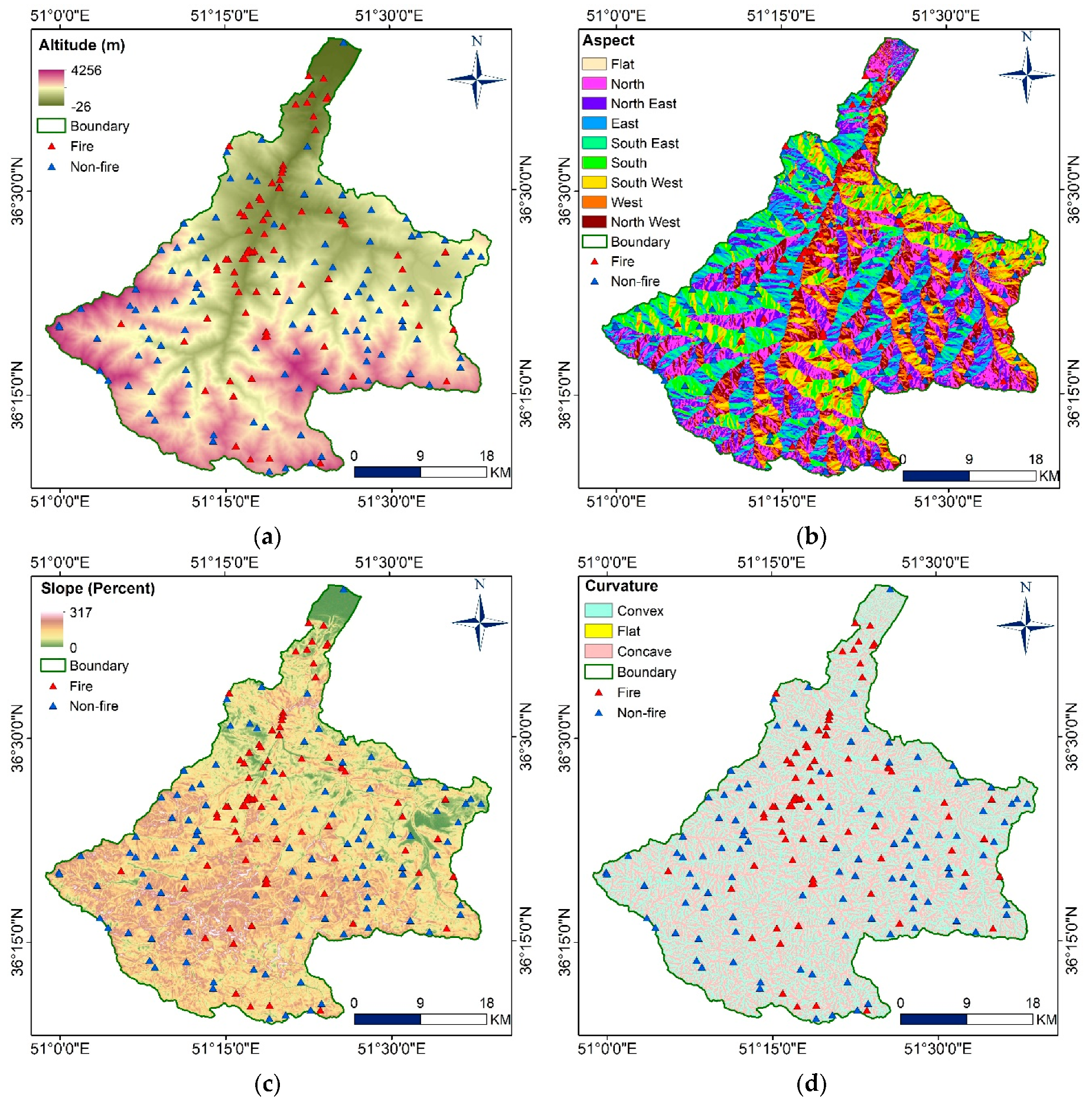
| Conditioning Factor | Source | Impact |
|---|---|---|
| Altitude | ASTER DEM | Controls the microclimate in terms of vegetation distribution, composition and flammability. |
| Aspect | ASTER DEM | Influences the local climate of the slope with respect to solar insolation, wind moisture content, etc. The hill side facing away from the direct sunshine usually retain more moisture supporting vegetation greenness and vigor. |
| Slope | ASTER DEM | Slope regulates vegetation distribution and composition, with high impact on the direction in which the fire rage and the speed at which it spreads, particularly at steep slope. |
| Curvature | ASTER DEM | Curvature indicates convergence or divergence of water in the landscape simultaneously with respect to downhill flow interpreted as either negative, zero or positive curvature. Negative curvature represents concave flow channel, zero curvature shows flat surfaces while positive curvature depicts convex flow waterway. |
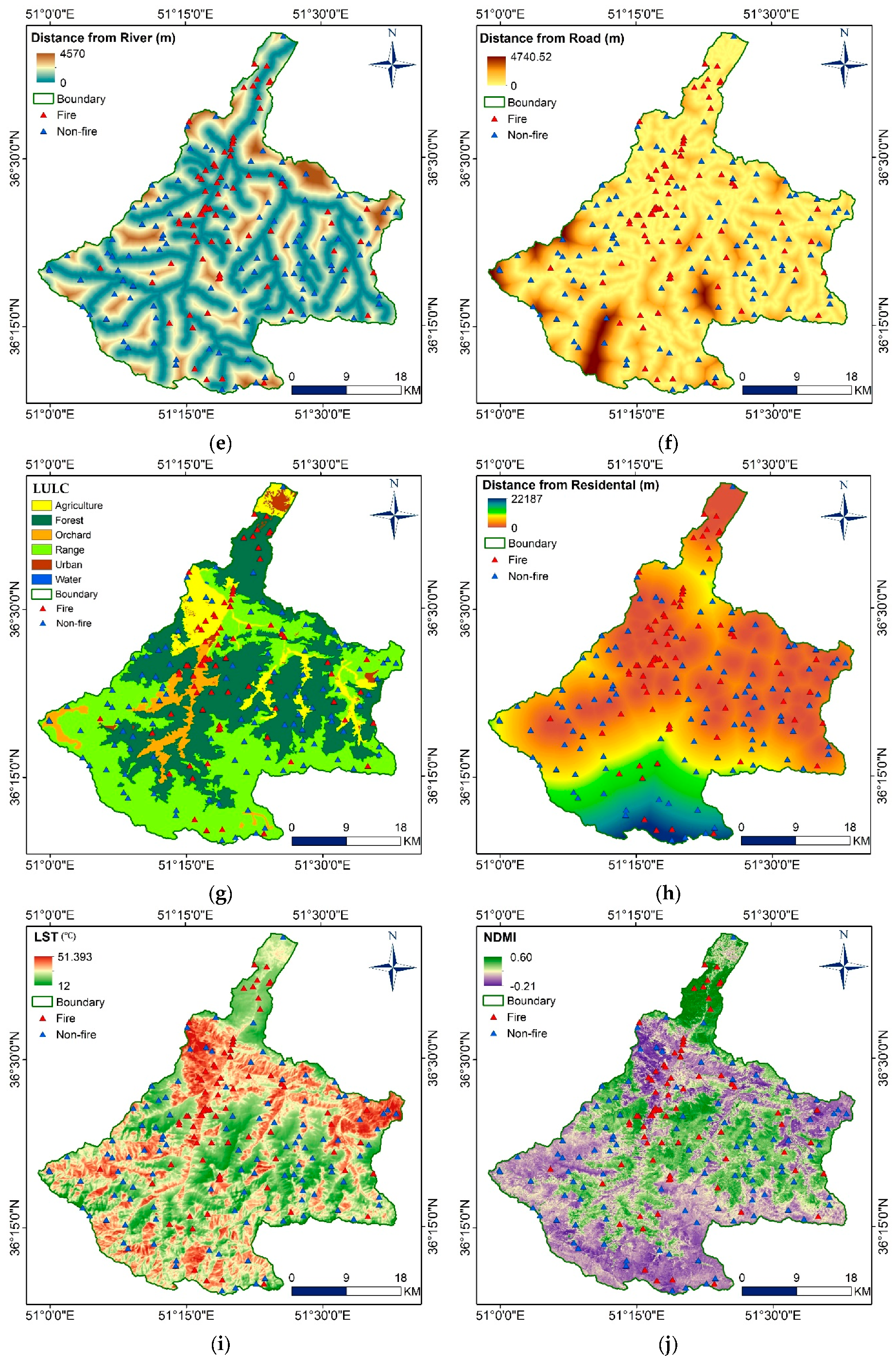
| Distance from river | GIS data | Vegetation close to rivers tend to be more greenish and healthier. Providing fuel for wildfire. However, moisture content in the vegetation could insulate inflammability. |
| Distance from road | GIS data | Roads provide accessibility to forests and consequently forest fire initiation through human activities. |
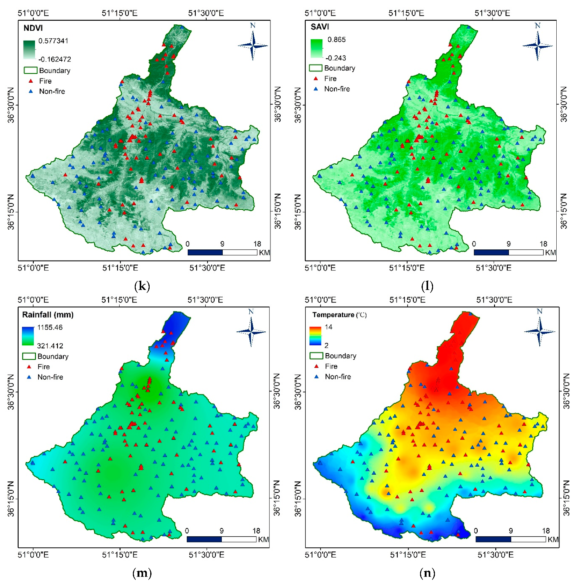
| NDVI | Landsat 8 OLI | It measures vegetation surface cover and density which indicates availability of fuel for fire spreading. |
| SAVI | Landsat 8 OLI | It measures vegetation amount, vigor and cover of greenness as indicators of flammability or otherwise of the area. |
| NDMI | Landsat 8 OLI | Moisture content of stressed vegetation fuel forest fire. NDMI measures the stress level and consequently degree of flammability. |
| LULC | Landsat 8 OLI | Describes the various use the land is put into and the activities involved, including fuel types and level of exposure to fire. |
| Distance from residential | LULC | The further away forest is to residential areas the lesser its vulnerability to fire occurrence. |
| LST | Landsat 8 OLI | Shows surface heat variation and its contribution to the spread of fire |
| Temperature | Meteorological data | Influences atmospheric air mass which controls relative humidity, air mass and soil moisture content. |
| Rainfall | Meteorological data | Increases the soil moisture and supports vegetation greenness that decreases the rage and spread of forest fire. |
| Row | Variables | VIF | Tolerance |
|---|---|---|---|
| 1 | Altitude | 3.08 | 0.32 |
| 2 | Slope | 1.51 | 0.66 |
| 3 | Aspect | 1.10 | 0.91 |
| 4 | Curvature | 1.19 | 0.84 |
| 5 | Distance from river | 1.84 | 0.54 |
| 6 | Distance from road | 1.54 | 0.65 |
| 7 | Distance from residential | 2.12 | 0.57 |
| 8 | LULC | 1.90 | 0.53 |
| 9 | LST | 3.26 | 0.31 |
| 10 | NDMI | 3.95 | 0.25 |
| 11 | NDVI | 4.23 | 0.24 |
| 12 | SAVI | 3.06 | 0.33 |
| 13 | Rainfall | 1.41 | 0.71 |
| 14 | Temperature | 2.48 | 0.40 |
| Models | Resampling | Stage | Evaluate Parameters | ||||
|---|---|---|---|---|---|---|---|
| Sensitivity | Specificity | NPV | PPV | AUC | |||
| MARS | non | Train | 0.72 | 0.75 | 0.73 | 0.71 | 0.83 |
| Test | 0.65 | 0.74 | 0.70 | 0.69 | 0.78 | ||
| 5 fold CV | Train | 0.84 | 0.86 | 0.88 | 0.83 | 0.92 | |
| Test | 0.77 | 0.77 | o.79 | 0.75 | 0.88 | ||
| 10 fold CV | Train | 0.88 | 0.93 | 0.92 | 0.91 | 0.94 | |
| Test | 0.74 | 0.86 | 0.79 | 0.82 | 0.90 | ||
| bootstrap | Train | 0.85 | 0.89 | 0.86 | 0.84 | 0.91 | |
| Test | 0.71 | 0.77 | 0.75 | 0.73 | 0.86 | ||
| optimism bootstrap | Train | 0.89 | 0.93 | 0.93 | 0.91 | 0.93 | |
| Test | 0.77 | 0.80 | 0.80 | 0.77 | 0.83 | ||
| SVM | non | Train | 0.78 | 0.86 | 0.88 | 0.91 | 0.92 |
| Test | 0.65 | 0.83 | 0.75 | 0.77 | 0.82 | ||
| 5 fold CV | Train | 0.79 | 0.86 | 0.87 | 0.90 | 0.92 | |
| Test | 0.65 | 0.83 | 0.75 | 0.77 | 0.82 | ||
| 10 fold CV | Train | 0.93 | 0.92 | 0.96 | 0.94 | 0.97 | |
| Test | 0.84 | 0.83 | 0.85 | 0.81 | 0.89 | ||
| bootstrap | Train | 0.86 | 0.92 | 0.91 | 0.89 | 0.95 | |
| Test | 0.77 | 0.80 | 0.80 | 0.77 | 0.87 | ||
| optimism bootstrap | Train | 0.87 | 0.82 | 0.81 | 0.86 | 0.92 | |
| Test | 0.84 | 0.74 | 0.74 | 0.84 | 0.84 | ||
| BRT | non | Train | 0.79 | 0.84 | 0.79 | 0.84 | 0.91 |
| Test | 0.74 | 0.83 | 0.78 | 0.79 | 0.87 | ||
| 5-fold CV | Train | 0.94 | 0.95 | 0.97 | 0.96 | 0.98 | |
| Test | 0.87 | 0.88 | 0.89 | 0.87 | 0.90 | ||
| 10-fold CV | Train | 0.95 | 0.95 | 0.98 | 0.97 | 0.98 | |
| Test | 0.84 | 0.83 | 0.85 | 0.S81 | 0.90 | ||
| bootstrap | Train | 0.96 | 0.94 | 0.98 | 0.93 | 0.98 | |
| Test | 0.87 | 0.80 | 0.87 | 0.79 | 0.90 | ||
| optimism bootstrap | Train | 0.98 | 0.97 | 0.99 | 0.98 | 0.99 | |
| Test | 0.87 | 0.83 | 0.89 | 0.82 | 0.91 | ||
| Susceptibility Class | Models | |||||
|---|---|---|---|---|---|---|
| 10-Fold CV MARS | 10-Fold CV SVM | Optimism Bootstrap BRT | ||||
| Area (Km2) | Area (%) | Area (Km2) | Area (%) | Area (Km2) | Area (%) | |
| Very Low | 132.01 | 8.09 | 301.96 | 18.51 | 241.44 | 14.80 |
| Low | 320.71 | 19.66 | 447.21 | 27.41 | 425.78 | 26.1 |
| Moderate | 479.41 | 29.39 | 387.32 | 23.74 | 426.26 | 26.13 |
| High | 468.11 | 28.69 | 284.25 | 17.42 | 326.53 | 20.02 |
| Very High | 231.1 | 14.17 | 210.6 | 12.91 | 211.33 | 12.95 |
| No | Variables | Value | % Importance |
|---|---|---|---|
| 1 | Altitude | 33.77 | 16.8 |
| 2 | Distance from river | 26.25 | 13.0 |
| 3 | Rainfall | 21.71 | 10.8 |
| 4 | Distance from residential | 18.09 | 9.0 |
| 5 | Curvature | 17.19 | 8.5 |
| 6 | NDMI | 14.07 | 7.0 |
| 7 | Temperature | 13.76 | 6.8 |
| 8 | Aspect | 12.87 | 6.4 |
| 9 | Distance from road | 12.06 | 6.0 |
| 10 | LST | 11.94 | 5.9 |
| 11 | NDVI | 7.56 | 3.8 |
| 12 | Slope | 6.78 | 3.4 |
| 13 | LULC | 3.81 | 1.9 |
| 14 | SAVI | 1.43 | 0.7 |
Publisher’s Note: MDPI stays neutral with regard to jurisdictional claims in published maps and institutional affiliations. |
© 2020 by the authors. Licensee MDPI, Basel, Switzerland. This article is an open access article distributed under the terms and conditions of the Creative Commons Attribution (CC BY) license (http://creativecommons.org/licenses/by/4.0/).
Share and Cite
Kalantar, B.; Ueda, N.; Idrees, M.O.; Janizadeh, S.; Ahmadi, K.; Shabani, F. Forest Fire Susceptibility Prediction Based on Machine Learning Models with Resampling Algorithms on Remote Sensing Data. Remote Sens. 2020, 12, 3682. https://doi.org/10.3390/rs12223682
Kalantar B, Ueda N, Idrees MO, Janizadeh S, Ahmadi K, Shabani F. Forest Fire Susceptibility Prediction Based on Machine Learning Models with Resampling Algorithms on Remote Sensing Data. Remote Sensing. 2020; 12(22):3682. https://doi.org/10.3390/rs12223682
Chicago/Turabian StyleKalantar, Bahareh, Naonori Ueda, Mohammed O. Idrees, Saeid Janizadeh, Kourosh Ahmadi, and Farzin Shabani. 2020. "Forest Fire Susceptibility Prediction Based on Machine Learning Models with Resampling Algorithms on Remote Sensing Data" Remote Sensing 12, no. 22: 3682. https://doi.org/10.3390/rs12223682
APA StyleKalantar, B., Ueda, N., Idrees, M. O., Janizadeh, S., Ahmadi, K., & Shabani, F. (2020). Forest Fire Susceptibility Prediction Based on Machine Learning Models with Resampling Algorithms on Remote Sensing Data. Remote Sensing, 12(22), 3682. https://doi.org/10.3390/rs12223682