Article

Early ICESat-2 on-orbit Geolocation Validation Using Ground-Based Corner Cube Retro-Reflectors

1
Applied Research Laboratories, University of Texas at Austin, Austin, TX 78712, USA
2
National Aeronautics and Space Administration, Goddard Space Flight Center, Greenbelt, MD 20771, USA
3
University of Maryland, College Park, MD 20742, USA
*
Author to whom correspondence should be addressed.
Remote Sens. 2020, 12(21), 3653; https://doi.org/10.3390/rs12213653
Submission received: 1 October 2020 / Revised: 1 November 2020 / Accepted: 5 November 2020 / Published: 7 November 2020

Abstract

:
The Ice, Cloud and Land Elevation Satellite-2 (ICESat-2), an Earth-observing laser altimetry mission, is currently providing global elevation measurements. Geolocation validation confirms the altimeter’s ability to accurately position the measurement on the surface of the Earth and provides insight into the fidelity of the geolocation determination process. Surfaces well characterized by independent methods are well suited to provide a measure of the ICESat-2 geolocation accuracy through statistical comparison. This study compares airborne lidar data with the ICESat-2 along-track geolocated photon data product to determine the horizontal geolocation accuracy by minimizing the vertical residuals between datasets. At the same location arrays of corner cube retro-reflectors (CCRs) provide unique signal signatures back to the satellite from their known positions to give a deterministic solution of the laser footprint diameter and the geolocation accuracy for those cases where two or more CCRs were illuminated within one ICESat-2 transect. This passive method for diameter recovery and geolocation accuracy assessment is implemented at two locations: White Sands Missile Range (WSMR) in New Mexico and along the 88°S latitude line in Antarctica. This early on-orbit study provides results as a proof of concept for this passive validation technique. For the cases studied the diameter value ranged from 10.6 to 12 m. The variability is attributed to the statistical nature of photon-counting lidar technology and potentially, variations in the atmospheric conditions that impact signal transmission. The geolocation accuracy results from the CCR technique and airborne lidar comparisons are within the mission requirement of 6.5 m.

Graphical Abstract

1. Introduction

The Ice, Cloud and land Elevation Satellite-2 (ICESat-2) launched in September 2018 and was placed in near polar orbit to measure global heights. Similar to its predecessor, ICESat (2003–2009), the primary scientific goal of ICESat-2 is to collect the critical measurements needed to better understand climate and climate processes [1,2]. These critical measurements are focused on the Polar Regions as they create the ability to derive ice sheet mass balance [3], and sea ice thickness [4]—aspects that indicate controlling mechanisms in climate dynamics [5]. Additionally, ICESat-2 provides heights for vegetation and land surfaces that indicate carbon stock and biomass while atmospheric and ocean measurements contribute to a comprehensive understanding of climate system interactions [6].
ICESat-2 carries a photon counting laser altimeter, ATLAS (Advanced Topographic Laser Altimeter System), to provide range measurements from space. These range measurements in concert with the satellite precision pointing and positioning information produce a geolocation and elevation for photon events detected by ATLAS. As indicated by the “photon counting” description of ATLAS, the signal detection sensitivity is at a single photon level which provides an operational advantage for lower power laser requirements and high repetition rates [7]. ATLAS produces a 532 nm laser pulse at 10 kHz. The single pulse is parsed into 6 separate beams, configured into three beam pairs, each containing a tandem of low and high relative energies. The beam pairs are separated by ~3.3 km in the across-track direction on the surface and 90 m between the pair components. This configuration is specifically designed to disentangle elevation change from surface slope (local and regional) while the energy variation increases the dynamic range of the instrument’s detection response to surface reflectance. The spacecraft’s mean orbital altitude is 496 km (±6 km) which creates the scenario of illuminating the surface of the Earth every 0.7 m along track (a pulse every 0.1 msec at ~7 km/sec) with expected footprint diameter of less than 17 m based on the pre-launch design specification. The diameter of the footprint is defined as the spatial extent of the laser energy illumination on the surface of the Earth. ATLAS records the arrival time of photons to less than a billionth of a second. These photon arrival times are aligned with the appropriate time of the transmitted laser pulse to assign each photon to a particular laser footprint on the Earth. Although the photon counting technology is producing aggregates of along-track measurements instead of elevations for individual laser pulses, the diameter does contribute significantly to horizontal and vertical resolution of the features within the footprint on the surface [8].
The scientific goals of the mission governed not only the attributes of the instrumentation relative to footprint diameter, data rates, measurement resolution and spatial coverage but also the operational implementation plans and the methodologies for computing the geophysical data products [9]. Each of the geophysical products are designated with the prefix “ATL” and a unique number. The geolocated photons are a Level 2a product-designated as ATL03. The surface specific products are Level 3a and include ATL06-ATL13 for land ice, sea ice, land/vegetation, ocean, atmosphere and inland water. The mission requirement for ATL03 geolocation accuracy is 6.5 m [2] representing the capability to resolve a measured geodetic position among the contribution of errors from the precision orbit and pointing determination processes. Since ATL03 is the input data for all of the higher-level data products, any errors in the geolocation will propagate forward to these surface specific Level 3a surface interpretations (static and dynamic). Here, we present a method for validating the horizontal position accuracy of ICESat-2 using corner cube retro-reflector (CCR) arrays and high-resolution reference data. The strategy of using passive ground-based methods for geolocation validation was investigated for the original ICESat mission [10,11] and recently studied for the application to the contemporary mission [12]. These CCRs provide an independent measure of footprint level positioning, the laser footprint diameter on the surface, insight into the pointing control of the observatory and overall instrument performance. The comparison to reference data such as airborne lidar gives another independent assessment of the satellite horizontal geolocation accuracy and also provides confirmation of the deterministic solutions derived from the CCR concept presented here. Ultimately, the goal of this work is to provide a proof of concept for small diameter ground-based optics as a means for space-based lidar geolocation validation while also proving that the satellite is meeting the ±45 m mission requirement for pointing control. The next section of the paper will provide the details of the CCR selection process specific to ICESat-2 characteristics, the approach for analyzing the signatures and the implementation of the technique at two test sites. The following section will present the results of the three satellite overpasses and provide discussion on the variability between each case. Finally, the paper will provide conclusions on how this technique should move forward with respect to geolocation validation and footprint diameter assessment.

2. Materials and Methods

2.1. Corner Cube Retro-Reflectors

CCR analysis started in the early 1970s with the expectation that they would prove useful for both lunar laser ranging and satellite laser ranging given their specific reflective capabilities [13,14,15]. The CCR is a unique component that provides a reflection along the initial energy angle of incidence, somewhat mimicking a specular reflection as opposed to a diffuse return. Chang et al. [16] studied the far-field diffraction pattern for corner cubes, using methods presented by Fraunhofer years earlier for circular apertures. This theoretical analysis was used to determine the appropriate size CCR for both ICESat and ICESat-2 mission use cases, with the implementation of putting CCR arrays on the Earth’s surface for independent space-based lidar geolocation validation [12].
The CCR diameter selection is a function of the wavelength, distance from the aperture (e.g., altitude of the satellite), and energy level of the laser. The derived strength of the signal return is proportional to the radius of the CCR, which means larger corner cubes reflect larger signal levels back to the satellite receiver. However, as the CCR diameter increases, the central diffraction disk of returned energy becomes smaller (e.g., diameter of disk is inversely proportional to diameter of the CCR). The Fraunhofer diffraction disk diameter is important in satellite applications as it requires consideration in context of spacecraft velocity aberration. If the velocity aberration value does not converge with the reflected disk diameter, the signal will fall outside of the receiver telescope field of view. In this situation, there is a chance to receive signal from the outer lobes of the Fraunhofer diffraction pattern but it is much less than the signal in the central disk that may or may not be an adequate return given atmospheric scattering and other optical losses [14]. The theoretical CCR size selection for ICESat-2 (wavelength and energy levels) was determined as a range of 6 to 8 mm diameters. This diameter range mitigates the issues with velocity aberration and yet provides an acceptable signal level given the estimated 60% atmospheric transmission each way, a 20% quantum efficiency and 50% detector efficiency [9]. In contrast, the ICESat mission successfully used a 12 mm diameter CCRs to supply both a geolocation accuracy assessment [11] as well as a signature tag for timing accuracy validation [10].
In preparation for ICESat-2 CCR validation, studies using the ATLAS airborne engineering testbed, MABEL (Multiple Altimeter Beam Experimental Lidar) [12] were conducted. The studies revealed that the CCR approach could provide an independent validation of geolocation despite the operational and technical differences between the ICESat’s full-waveform, high-energy lidar technology and the photon-counting technology of MABEL and ICESat-2. However, the analysis of the return signatures required a new approach to accommodate the transition from a single large footprint illumination of multiple corner cubes (ICESat) to the ICESat-2/MABEL illumination of one CCR with multiple laser shots. Understanding multiple laser illuminations of a single CCR for geolocation validation requires a geometric analysis of relative positioning of the CCR and footprint centerline (diameter) and knowledge of the ICESat-2 geolocation determination process.
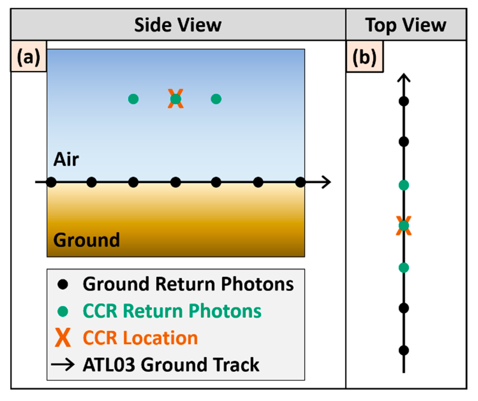
A theoretical scenario for a CCR position exactly aligned with the centerline of the laser footprint would nominally provide a signal every 0.7 m with a timestamp step of 0.1 msec (10 kHz) through the entire length of the ICESat-2 footprint diameter. If the diameter is equal to 17 m (pre-launch best estimate) then in an ideal case this would provide at least one CCR reflected photon from 24 individual laser shots over 2.4 msec. These points appear to be successive single, or multiple, photon detections along-track (at 0.1 msec delta timestamps) with an elevation representative of the height of the CCR above the surface. A conceptual view from a horizontal perspective of the CCR signal and associated ground return elevations is shown in Figure 1a, each point representing a geolocated photon, black specific to terrain or ground photons and green from the CCR. The red X represents the actual position of the CCR. The top view of the CCR returns, in Figure 1b, show the alignment, horizontally, of the CCR and ground returns despite the difference in elevation. This alignment brings an interesting challenge to the CCR signature analysis in that any detected photon associated with a specific laser shot will be geolocated at the geometric centroid or “bounce point” regardless of spatial separation between that reflection point source and the footprint centroid. As such, if the position of the CCR is coincident to the footprint centerline, then the CCR signature requires no additional interpretation with respect to comparing the ATL03 geolocation to the known position of the CCR.
Keeping the focus on the scenario of the CCR and along-track ATL03 alignment in Figure 1, 
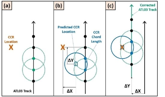
Figure 2 presents a time lapse representation of multiple footprint illuminations for one optical component and the expected detected photons. The dotted green circles are the individual laser footprints based on the ATL03 geolocated centroids and the blue circles are associated with statistical determination of the footprint location relative to the CCR position. Although not to scale, the diagram illustrates the collection of CCR detected signals as they initiate with the leading edge of the first relevant laser shot (Figure 2b) and ends with the trailing edge of the final spot (Figure 2f), in this case, the third footprint. Figure 2f highlights the recovered chord length (along-track distance of the CCR photons) as equivalent to the diameter of the laser footprint. The mid-point of the CCR signature is directly compared to the known CCR position to assess the ATL03 geolocation accuracy in both along-track (ΔY) and across track (ΔX) directions. In the case of Figure 2, the geolocation has no error (ΔX = ΔY = 0) as the predicted mid-point of the CCR signature matches exactly with the known CCR coordinates. 
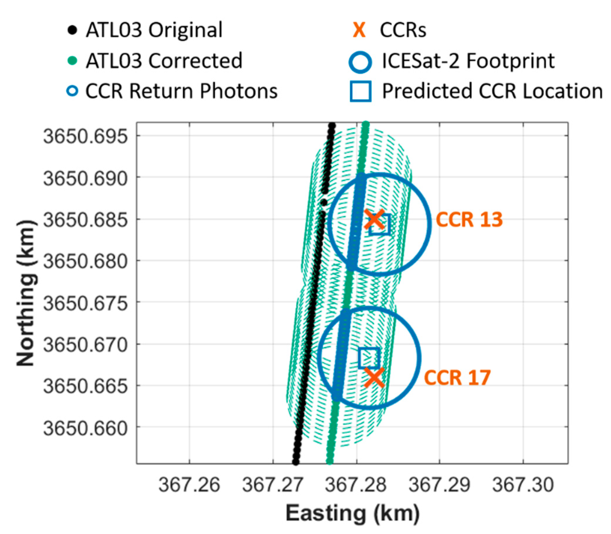
Figure 3 illustrates the case where the CCR is still aligned with the centerline but there is geolocation error in the data. In this example, the predicted CCR position (blue square) using the mid-point of the CCR signature is not equal to the actual CCR position (red X) such that ΔX and ΔY are the horizontal offsets and indicate the ATL03 geolocation accuracy.
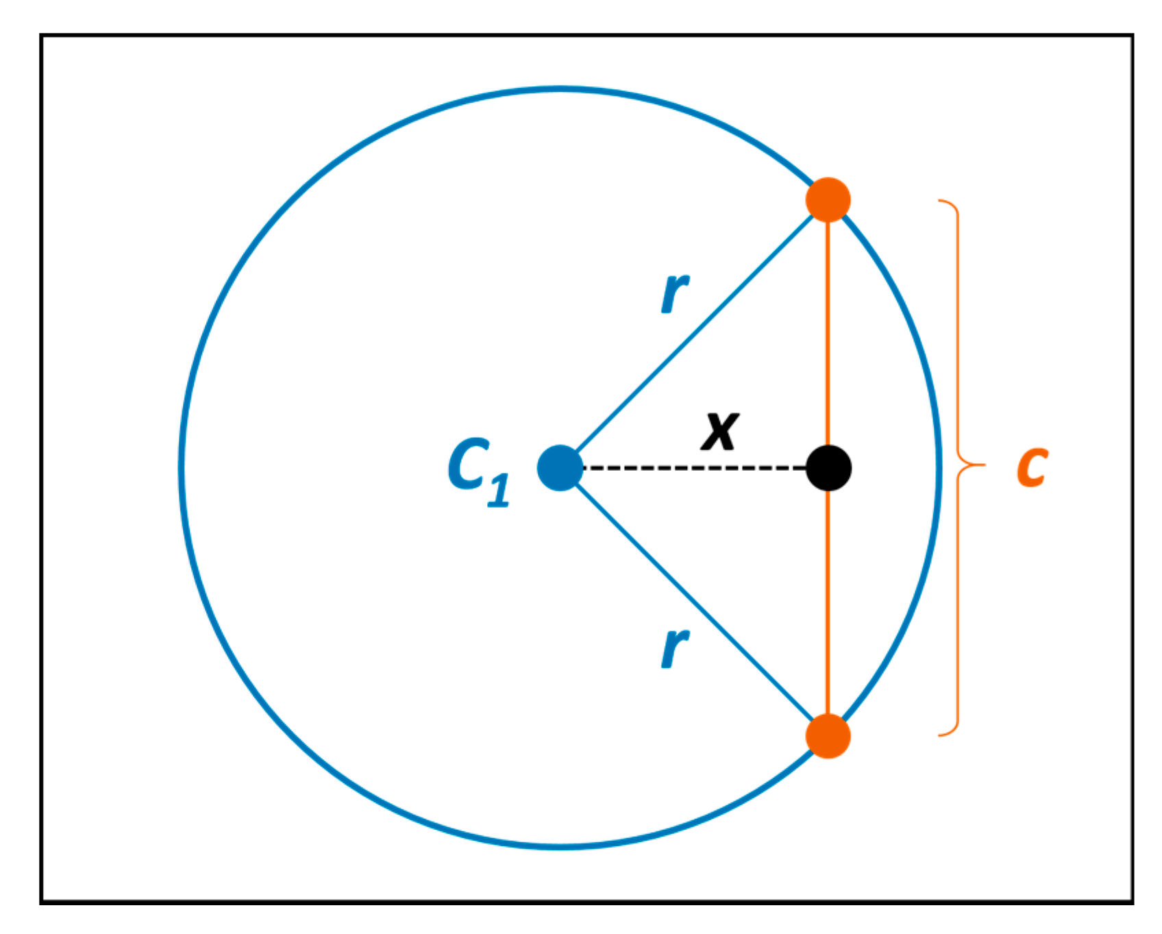
More complexity occurs when the CCR position and footprint centerline are not aligned. For those cases, the apparent along-track chord length of the CCR signature will decrease. This length will be inversely proportional to the across-track distance from the centroid of the footprint based on the geometry of a circle. Figure 4 provides the relative chord length (c) of the CCR signature when its position (black dot) is a distance (x) from the footprint center (C1). To determine the geolocation accuracy of the data, the horizontal offset between the CCR position and the footprint centroid must be calculated using simple geometry for a given footprint diameter and measured chord length.
Figure 5 depicts the scenario where the CCR and centerline are not aligned and there is a geolocation error. Similar to the other figures, the panel at the end of the time lapse of laser shots provides the results for the along-track (ΔY) and across-track offset (ΔX) between the predicted footprint centroid and the CCR position. This is the applicable approach used for the ICESat-2 CCR based geolocation validation moving forward.
An important detail in the geometric analysis for ATL03 geolocation validation using CCR arrays is the approach for systematic chord length extraction from ATL03 data to ensure statistical consistency for multiple overpasses and different ICESat-2 beams. Although the diagrams presented in Figure 1, Figure 2, Figure 3, Figure 4 and Figure 5 clearly show a very stark beginning and end of the CCR signature length in theory, the reality is much different given the variability with radiometric (signal strength) influences such as atmospheric attenuation, surface reflectance, solar background noise and beam energy. 
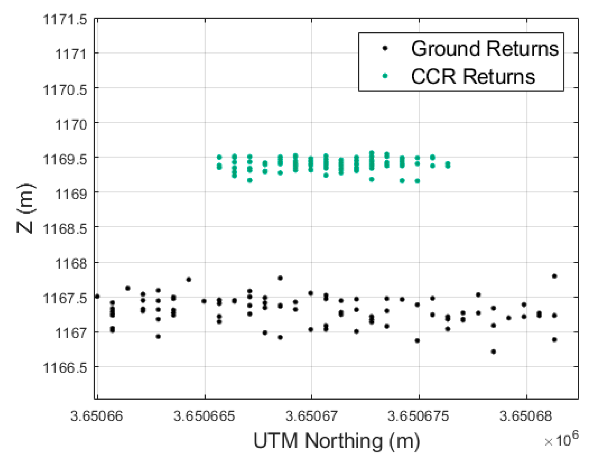
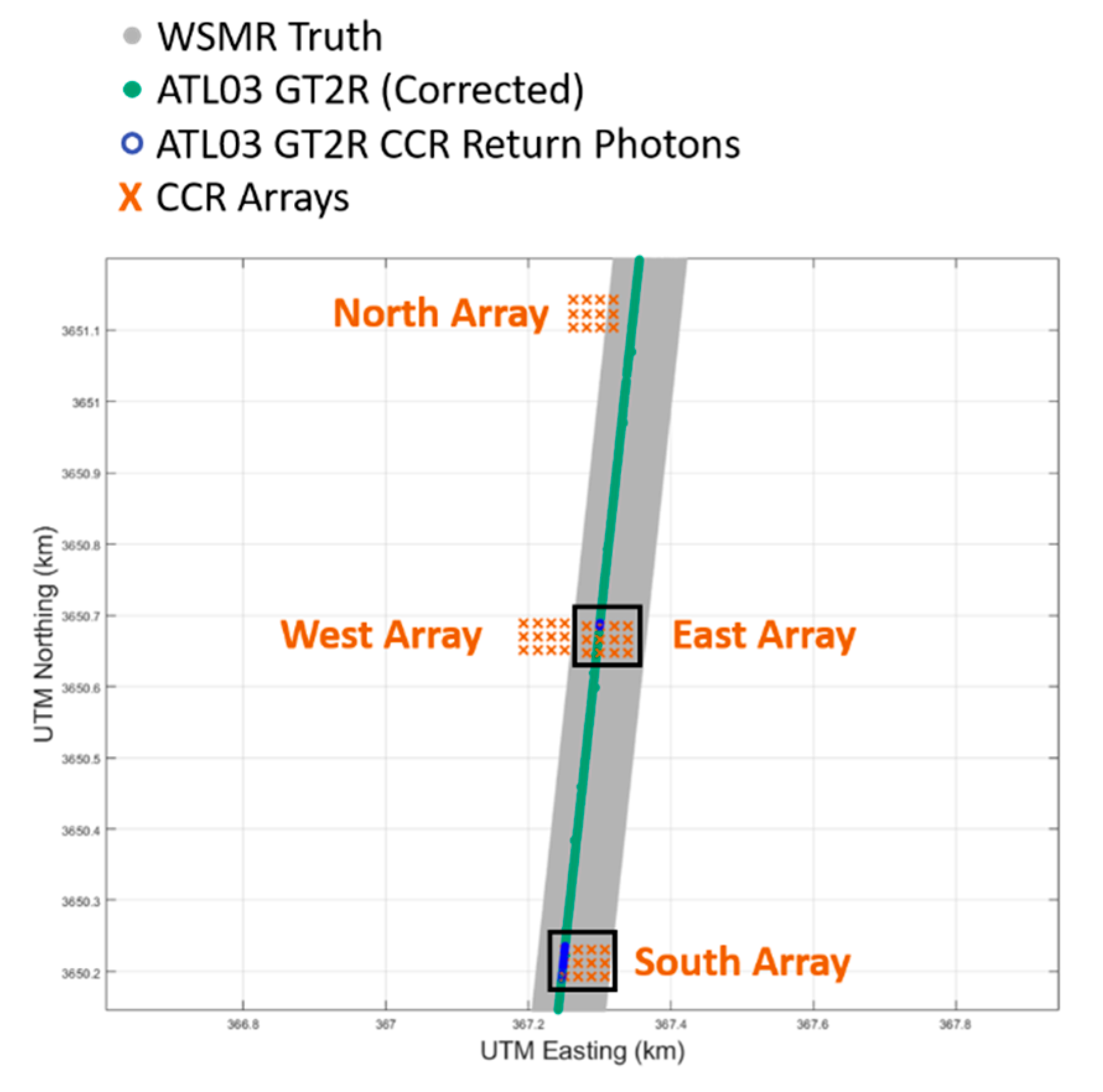
Figure 6 shows example CCR data from an ICESat-2 overpass collected at White Sands Missile Range (WSMR). The figure is a side view of the ATL03 geolocated point cloud, showing detected ground photons in black and CCR detected photons in green. Although not the case in this example, when heavy solar background noise is present, signal finding can be more difficult.
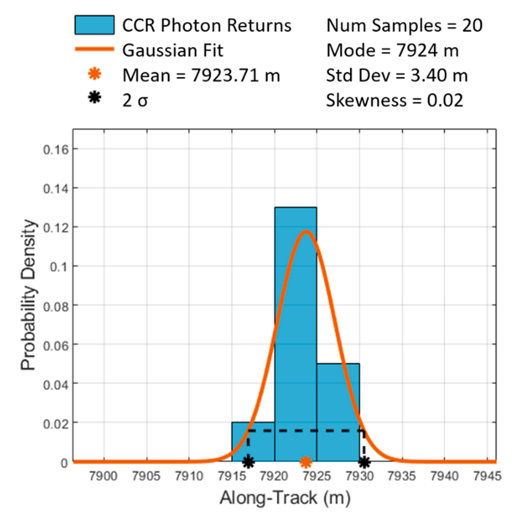
Typically, laser diameters are the equivalent to the 1/e2 Gaussian beam diameter; representative of 86.6% of the total energy spatial profile. It is entirely possible to detect CCR returns from outside of the 1/e2 boundary based on theoretical calculations, but those are more susceptible to radiometric losses. As such, the 1/e2 assumption provides standardization with the fact that the 1/e2 diameter is associated with a 2σ value of a Gaussian energy profile so the chord length extracted from the signature would mimic this estimation. 
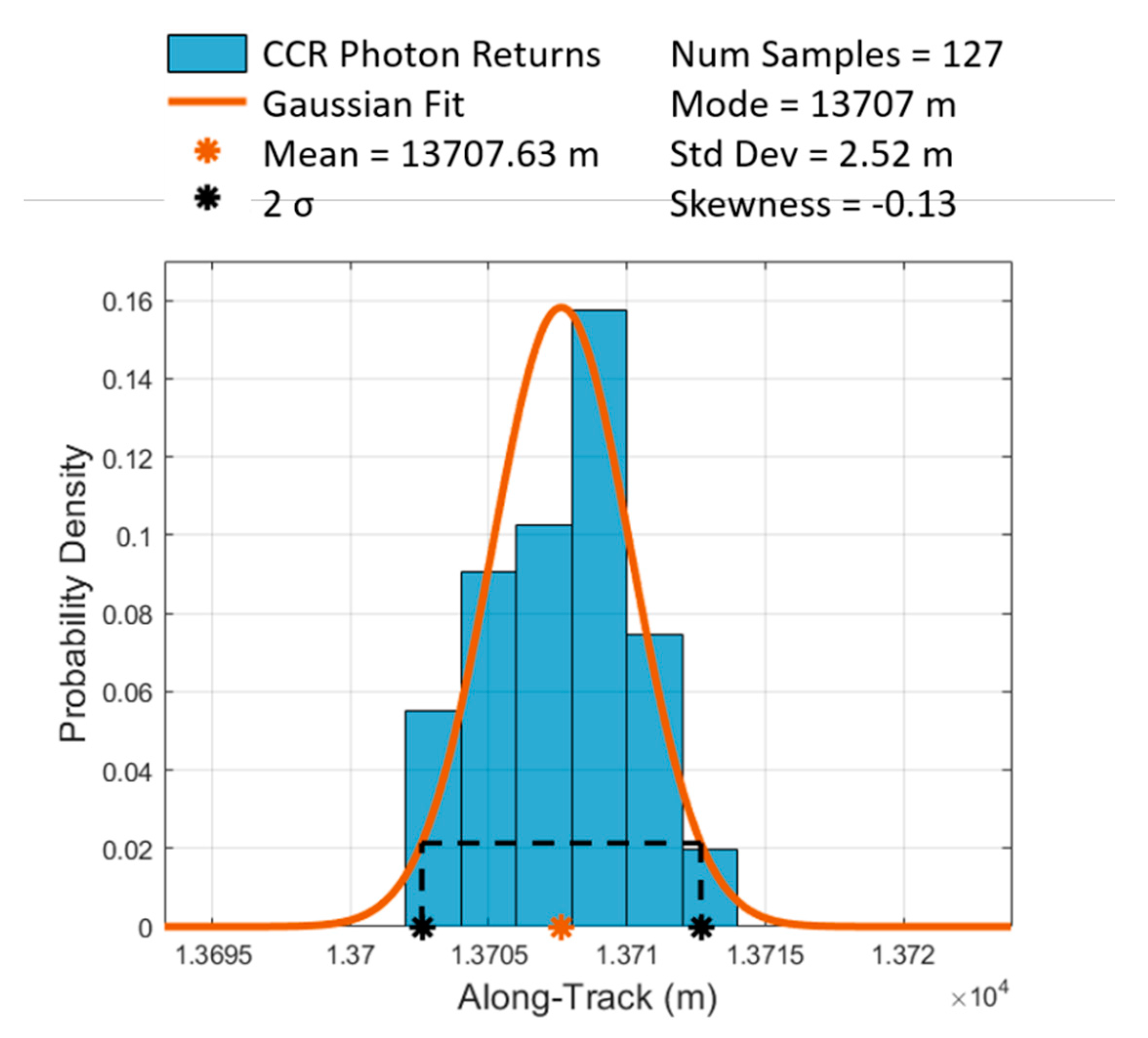
Figure 7 provides the statistical histogram representation of the CCR signature shown in Figure 6 and the corresponding Gaussian profile. Although the along-track distance for those data in Figure 6 is 10.1 m the 2σ value is 10.7 m. Pre-launch ATLAS laser measurements confirmed a Gaussian beam profile [17] but certainly the CCR distribution profiles are not a perfect Gaussian representation, particularly when the sample size of photons is relatively small. More appropriate distribution statistics can be explored as more satellite overpasses are captured. However, as a preliminary effort the Gaussian fits provide the means for exploring the efficacy of the technique and have skew values that are still considered approximately symmetric.
The CCR return photon chord length geometrically constrains the geolocation solution but only if the diameter is known to determine the distance of the CCR position relative to the centerline. Although pre-launch estimates of diameter exist there is no on-orbit method capable of confirming the true operational value. Furthermore, even if the diameter is known if there is only one CCR illuminated, the symmetry of the spot creates ambiguity as to if the CCR position is east or west of the centroid. The mitigation for these uncertainties is the collection of multiple CCR returns within one overpass. The analysis of the signals in concert create a unique scenario purely based on the relative geometry of the CCR positions in the array and chord lengths of the signal signatures. This creates a deterministic method for finding the effective diameter of the laser footprint and the geolocation simultaneously.
The comprehensive (diameter and geolocation accuracy) CCR analysis approach calculates both through an iterative process, varying the diameter and finding the best fit to the geometric constraints. 
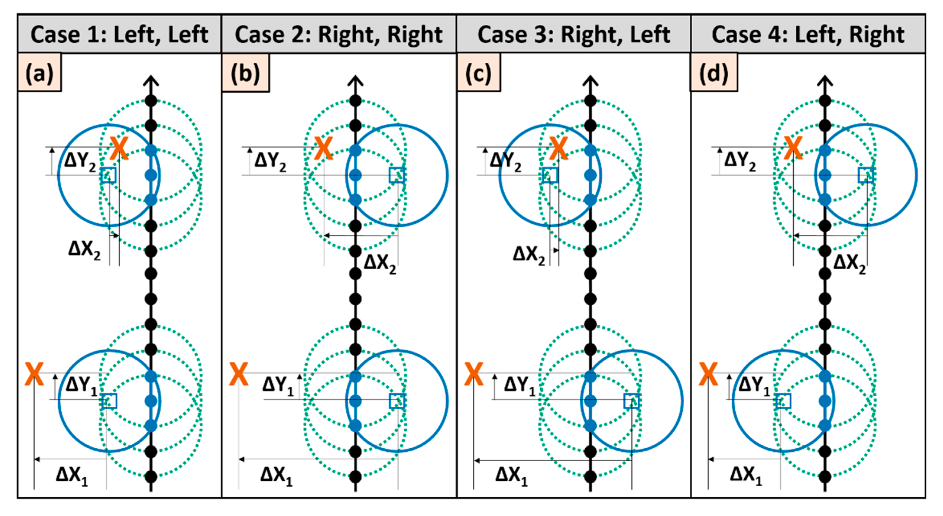
Figure 8 shows one iteration for diameter recovery for which the laser ground track passes to the east of two CCRs (panel 1). Starting with an initial estimate of footprint diameter, the algorithm determines the geolocation offsets (ΔX, ΔY) for each CCR signature. Since the goal is to determine one final geolocation offset for the track, the mean of the offset contributions from the individual CCRs is used, denoted as ΔXμ and ΔYμ in Panel 3 of Figure 8. To assess the geolocation solution, the root mean squared error (RMSE) between all centroid predictions and CCR positions is calculated with the idea that the minimum RMSE is representative of the best fit to the geometry. This process is performed for all possible footprint diameters at 10 cm increments from 5 to 20 m and repeated for all footprint configurations, e.g., the relative track position to the CCR positions. The number of configuration combinations is 2N, where N is the number of CCRs illuminated within one overpass. For the case presented in Figure 8, there will be four possible geometries evaluated for mean geolocation offset and RMSE of the solution for a given diameter (Figure 9). The lowest RMSE scenario will provide a final geolocation accuracy and estimate of the laser footprint diameter.

2.2. Ground-Based Validation Implementation: White Sands Missle Range (WSMR), New Mexico

The analysis to determine the precise location, configuration and orientation of the CCR arrays was based on the pre-launch details for ATLAS beam spacing on the surface and the planned reference ground tracks. The spacecraft orbit is inclined at 92° relative to the celestial equator which means 2° from a true polar orbit [2]. The inclination creates a 6.3° angle relative to a north/south orientation of the satellite ground tracks at the WSMR latitude. The ground track orientation is an important geometry consideration in the physical design of the CCR arrays in the hope to capture multiple CCR signatures for a beam pair (weak and strong) during a single overpass. The global design of the arrays uses the diamond pattern (Figure 10) created by the descending and ascending reference ground track intersections in nearest proximity of the target location and uses each of the four diamond vertices as a center point position for a local array. These four array locations coincide with the orange squares in Figure 10. Since the array design goal is to capture one of the three beam pairs during a single overpass, it is important to understand how the pairs are identified. For the three pairs, pair 1 is on the left side of the satellite relative to the direction of motion. The individual components within the pair are deemed Ground Track 1 left (GT1l) and Ground track 1 right (GT1r). The nadir beam pair is pair 2 and the pair to the right of the satellite direction of motion is pair 3. Those individual beams are GT2l, GT2r, GT3l, and GT3r, respectively. The array positions, in Figure 10, are designed to capture GTxl with the east and south array and GTxr with the north and west arrays for a descending pass. For an ascending pass the same configuration will capture GTxr with the east and north arrays and GTxl with the south and west respectively. The geographic distances of the arrays and the selected spacing of the CCRs within the arrays is provided in Figure 11.
Although one ICESat-2 reference ground track (RGT) is planned to directly pass over the arrays, additional ground tracks in near proximity will require the observatory to point off-nadir to this target of opportunity (TOO). TOOs can be implemented via uploaded instrument command files if not in violation of the operational limit of 5°. These off-nadir instances are important for validation studies as they often magnify errors or biases in the position or pointing determination solutions not normally observed during typical near-nadir pointing [18,19,20]. The success of a TOO is indicative of the observatory pointing control capability and confirms that the instrument command process, and on-board attitude control systems are working appropriately.
As previously discussed, the correlation of corner cube position and the resultant signal along-track chord length provides the opportunity to determine both the ground track’s positional offsets and the laser footprint diameter. However, there remains a need to appropriately identify which CCR belongs to a specific signature. If that information is unknown, it will be impossible to determine the appropriate geometric constraint. That said, if the CCR mount heights within an array are varied, any given linear (along-track) signal detection sequence is unique with respect to the vertical offsets within the array. Figure 11 depicts the array content in terms of individual mount heights, sufficiently populated so as to increase the likelihood of ICESat-2 ground track intersections and to support unambiguous determination of CCR ownership to those signatures in the ATL03 product.
The deployment of the CCR arrays was completed just prior to the satellite launch date to ensure they were assembled in time for early on-orbit validation but were not overly-exposed to environmental conditions that might degrade the optics unnecessarily. The CCRs were embedded in 0.4 m PVC caps customized to hold the 8 mm diameter optical components. These caps were placed on PVC pipes of variable length to adhere to the pattern shown in Figure 11: 0.75, 1.5, 2.3, and 3 m. These heights were chosen based on the vertical resolution within ATLAS, as they would provide distinct elevation separation from the surface as well from each other. Furthermore, none of these mount heights created significant logistical challenges associated with securing in place as taller poles are at risk of breaking or collapsing in the known environment experienced previously with the validation efforts for ICESat. The pipes were secured to the surface with partially submerged metal rebar and support wires. The position of each CCR was surveyed with differential Global Navigation Satellite System (GNSS) for a geolocation accuracy to within 1 m.
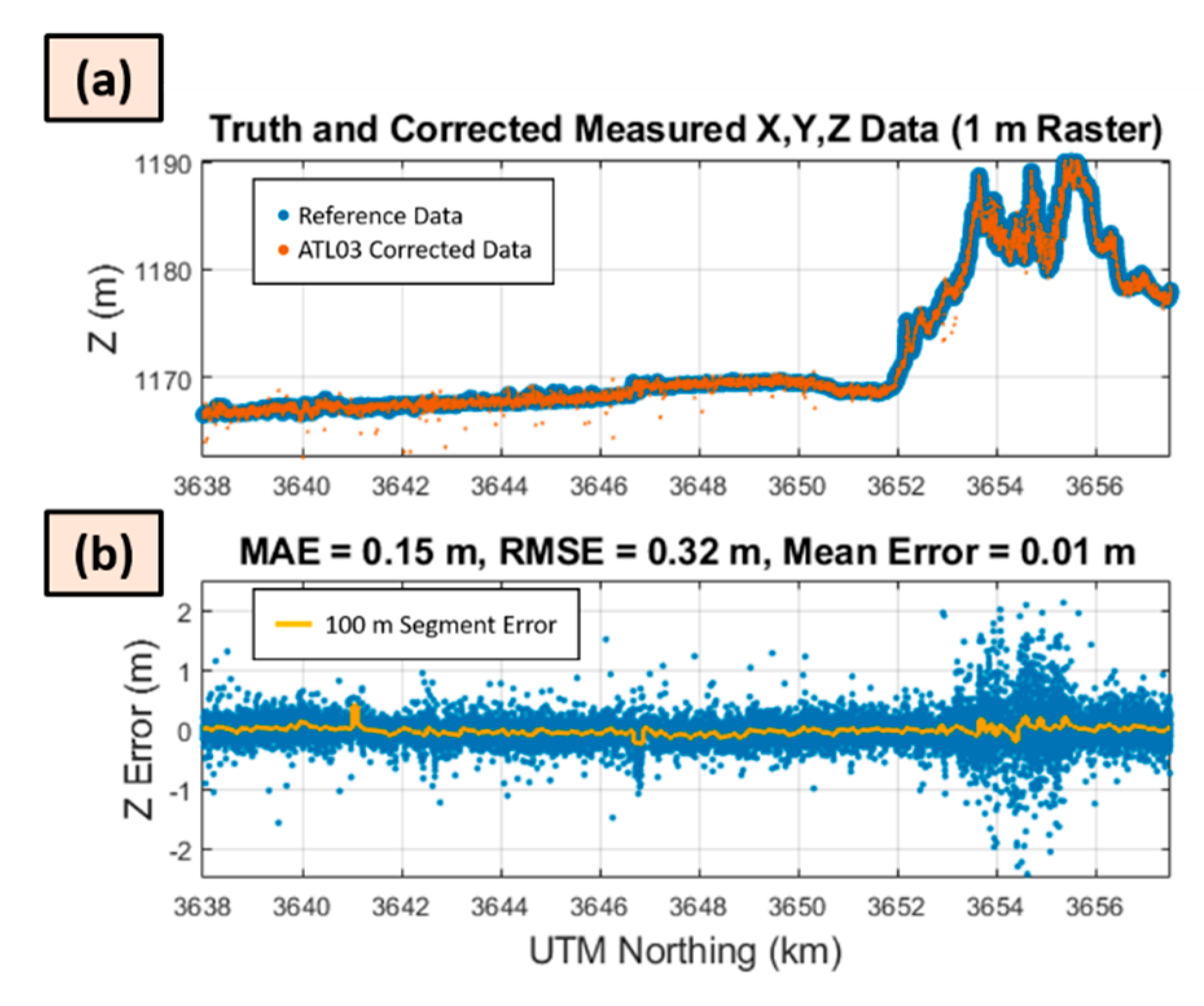
Another method for independent ICESat-2 geolocation validation can be accomplished by comparing the satellite data to known, high-resolution datasets. These “reference” surfaces provide accurate characterization of the region that can be directly compared to the ICESat-2 ATL03 elevations as well as the higher-level geophysical data products at variable length scales. The University of Texas at Austin Bureau of Economic Geology performed an airborne lidar survey over the region of WSMR within the broader range perimeter using a Leica Chiroptera lidar system and a high-resolution imager. The airborne collection acquired both near-infrared (NIR) and visible (green) data at ~10 pts/m2. Accuracy of the lidar dataset was enhanced using GNSS base-stations for data post processing. These receivers enabled differential solutions to produce the most accurate lidar measurement for surface characterization. Based on the effective post processing and the characteristics of the Leica system the airborne measurements provide, on average, better than 10 cm vertical accuracy and 1 m horizontal. The terrain is somewhat homogeneous at WSMR but there are distinct geophysical features within the scene that can be used as ground control, or reference points in the comparison to those relevant ICESat-2 transects across the region. This method provides an independent assessment of both the horizontal and vertical accuracy of the ATL03 product and was also planned to validate the results of the CCR proof of concept for geolocation validation.

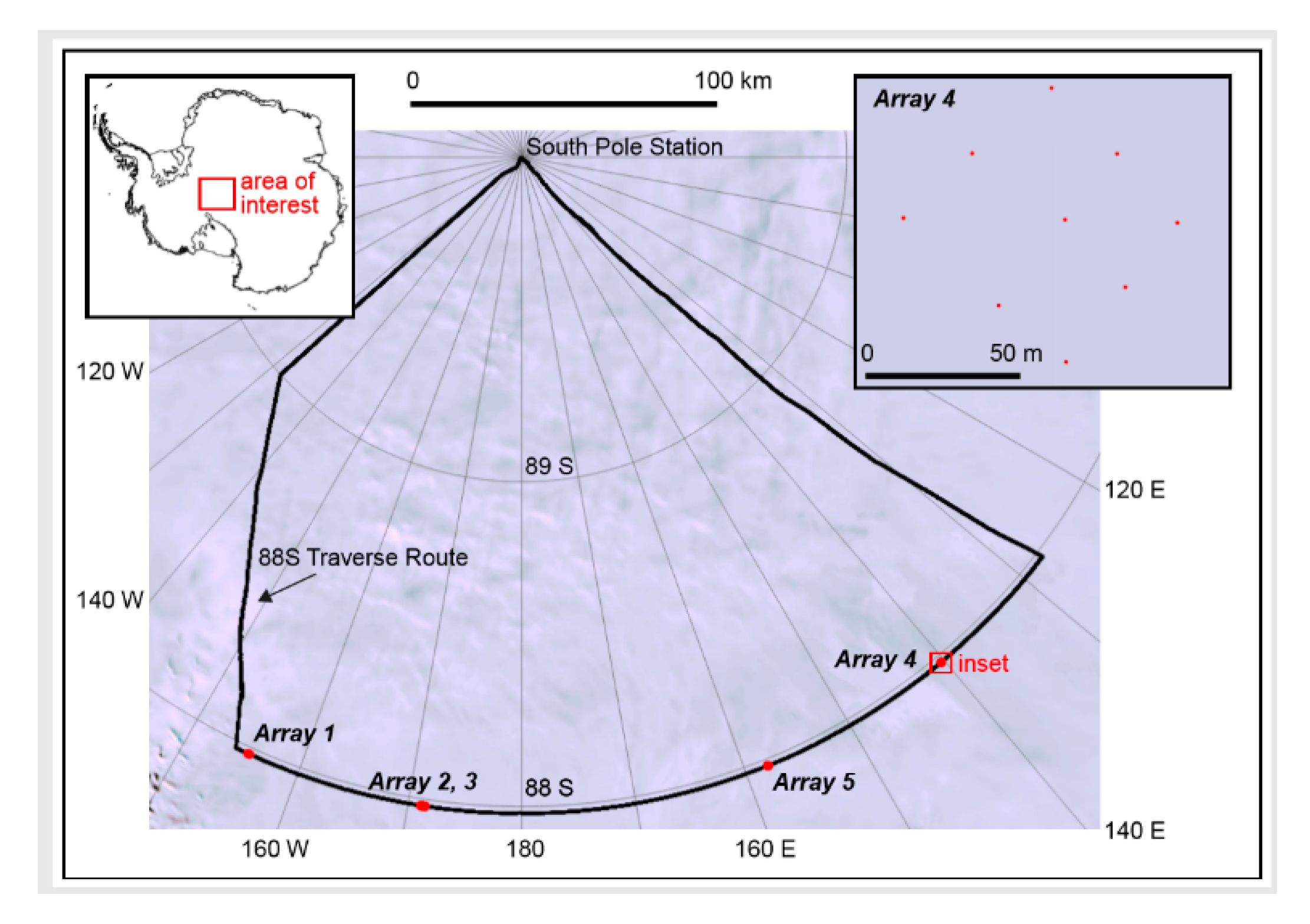
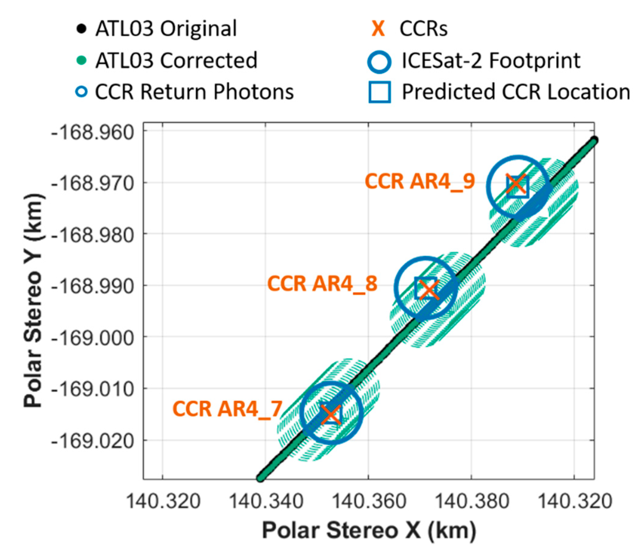
2.3. Ground-Based Validation Implementation: 88S Traverse

Since the validation efforts at WSMR provide assessment of the satellite measurement accuracy at a single northern-hemisphere point within the orbit, CCR arrays were also deployed along a portion of the 88° South (88S) line of latitude in Antarctica, where a large-scale ICESat-2 validation effort, referred to as the 88S Traverse, is underway [21]. Given that ICESat-2 has an orbital inclination of 92°, the orbits converge along 88S, making it a dense region of ground tracks and cross-over points.
A total of 5 small arrays were deployed along the 88S Traverse during the two different traverse seasons (2017–2018 and 2018–2019). The geographical location of the traverse and the CCR arrays are provided in Figure 12. The arrays contained anywhere from 4 to 9 CCRs and were mounted on bamboo poles using PVC caps. The bamboo poles varied in height from ~0.5 m to just under 2 m, in patterns such that a given CCR was distinguishable from the neighboring CCRs, similar to the concept of Figure 3. The spacing between the bamboo poles was ~30 m, such that the spacing was larger than the ICESat-2 expected footprint diameter ~17 m, but much smaller than the across-track spacing of the ICESat-2 beams (~90 m) and the mission requirement of spacecraft pointing control (45 m).
The positions of the bamboo poles were measured using kinematic GNSS methods and Precise Point Positioning post-processing techniques in a commercial software package [22]. Metal poles were also deployed in the center of each array to allow for easy resurveying of a single position of the array to assess horizontal movement of the arrays due to ice-sheet flow; the positions of the metal poles marking the centers of the arrays that were deployed during the first field season were resurveyed during the second season.
Revisiting and resurveying the arrays in the second season provided insight into the stability of this surface with respect to validation of both satellite ranging and the horizontal movement of the ice sheet (~0.3 m/year). The snow surface in this region is extremely flat on large length scales, varying by only 100 m over 300 km, but is relatively rough on short length scales. This roughness is associated with sastrugi, or fields of wind-driven ridges that are ~1 m high on ~10 m length scales. The position of sastrugi in the vicinity of our CCR arrays changed between seasons 1 and 2, as expected [23]; thus, during the second survey of the arrays, the relative heights of the bamboo poles changed non-uniformly. Most poles were still within the height range of ~0.5 m to just under 2 m; one bamboo pole was 0.48 m while another bamboo pole was anomalously low at 0.06 m. The horizontal displacements due to ice flow of five of the metal poles marking the centers of the arrays were extremely small, with a mean value 0.35 m. Thus, CCR arrays along the 88S Traverse are an excellent means of validation of horizontal accuracy and to assess the size of the ICESat-2 footprint, but these arrays are not ideal for the validation of satellite ranging as the pole heights are relative to the changing surface.

3. Results

3.1. White Sands Missile Range Airborne Lidar Comparison

The overpass on 2 November 2018 provided one of the first cases to investigate the ICESat-2 pointing control and geolocation accuracy. The TOO was implemented on reference ground track (RGT) #531, a descending pass that falls west of the validation site. For this pass the TOO command required a 3.41° off-nadir angle (31 km) which was performed through a roll maneuver to point left (east) of the sub-satellite point. The TOO targeted beam GT2r which is the middle pair’s right component, the strong spot for the +x spacecraft yaw orientation [3] at the time of the overpass. Although the beam did not illuminate a CCR array, analysis for ATL03 quality utilized positional offsets using the best fit to the airborne lidar reference surface. The results of the comparison initially were well outside the mission requirements but further calibration analysis on-orbit helped eliminate many of the errors and remove the biases. Comparison to the reference surface (1 m raster) at WSMR indicates −3 m along-track and 1 m across-track error in the geolocation reported in this test case. The thematic output of the automated comparison algorithm is shown in Figure 13 and the vertical error over the full transect at WSMR is provided in Figure 14. The thematic contours in Figure 13 show the optimization process as the ATL03 elevations are shifted in along-track and across-track directions to determine the best fit to the reference. The red dot, in Figure 13, indicates this best fit. The geolocation offset, or geolocation error, is the translational distance during the optimization.

3.2. Corner Cube Signatures at White Sands Missile Range

An overpass on 31 March 2019 provided the first successful CCR signal collection at WSMR with RGT #28, a descending pass to the east of the array location. The TOO required an observatory maneuver 2.4° off-nadir (21 km) from the sub-satellite point and placed the right beam (weak) in the middle pair (GT2r) on one CCR in the east array and two CCRs in the south array. The nadir view of the relative geometry for the ICESat-2 #28 RGT ATL03 along-track data and the four CCR arrays are shown in Figure 15. The ATL03 signal photons are green and the ATL03 signal photons attributed to the CCR reflections are blue.
Analysis of these signatures individually and collectively provides information on signal strength, laser spatial profile, and certainly, geolocation accuracy. Figure 16 shows the sequence of CCR signatures within the transect (elevation versus UTM northing). As observed in Figure 16, the heights of the illuminated CCRs moving south to north (left to right) are 1.01, 1.68, and 0.79 m. Coordinating these CCR heights in ATL03 with those approximated heights in the arrays confirms the CCR positions of those required for the geolocation and diameter retrieval process.
The 31 March WSMR data were analyzed using the methods described previously. The signal distribution and Gaussian function for one of the CCRs illuminated are shown in Figure 17, with a noticeable attenuation at the footprint boundaries where the energy levels are significantly lower. Using the chord lengths and iterative analysis with the geometric constraints the results it a footprint diameter of 10.6 m for this particular beam and environmental scenario. The centroid of the true geolocation is calculated based on the now known diameter and the chord length horizontal distance from the centerline of the footprint. The horizontal geolocation offsets were determined to be −1.8 m for both the along and across-track directions to produce a total horizontal geolocation accuracy to within 2.5 m (0.34 RMSE). Figure 18 illustrates the ATL03 data (black dots), the predicted location of the CCR relative to the footprint centroid based on the chord length (blue squares) and the ATL03 track correction based on the recovered geolocation offsets (green dots). Independent from the CCR approach for ICESat-2 geolocation error assessment is the error evaluation using the ATL03 data comparison to the WSMR airborne lidar survey. Comparison of the lidar reference data for the March overpass estimated a 2 m (RMSE 0.16 m) horizontal geolocation error. The comparison of the two results from the independent validation strategies confirms the fidelity of the CCR methodology for geolocation retrievals at WSMR and other locations, like 88S, where the surface is changing and/or reference data are not available.
Another overflight of WSMR on 28 September 2019 provided capture of the strong beam in the middle pair on the same track previously analyzed (RGT #28, GT2r). Although the same spot location (GT2r) as the previous overpass in March, the satellite had performed a yaw maneuver for the purpose of solar panel orientation which repositioned the strong and weak beam placement within the pair naming convention. The satellite was able to place the beam just 20 m from the intended TOO geodetic location requested. This particular pass was a daytime pass, and although the background noise level increased, the stronger beam energy provided significantly more signal than the weak beam delivered in March. Figure 19 illustrates the geometry of the track relative to the CCRs arrays; three distinct CCR signatures were identified in the data transect, one from the north array and two from the east. The geometry of the array with the apparent chord lengths of the CCR signatures gave a deterministic assessment of the footprint diameter to be 12 m (RMSE of 1.8 m).
Figure 20 shows the actual ATL03 data (black) and the adjusted positions based on the 12 m effective diameter, known locations of the two CCRs and the resulting geolocation offsets. This analysis concluded that geolocation accuracy of ATL03 is better than 5 m horizontal (−4 m across-track and 3 m along-track). In comparison, using the airborne lidar survey for geolocation accuracy assessment resulted in the same conclusion (−4 m across-track, 3 m along-track) which again confirms the fidelity of the CCR methodology for diameter and geolocation retrievals.

3.3. Corner Cube Signatures at 88S

Compared to the number of possible TOOs at WSMR, the 88S CCR arrays have more opportunities for illumination based on the spatial convergence of the reference ground tracks at this latitude. From many successful captures of CCR signatures, 10 December 2018 was one of special interest as it illuminated three targets within the AR4 array (Figure 12) on one RGT track (#1111). Figure 21 shows the location of this particular track and the corresponding locations of the CCRs responsible for the signal signature in the transect. This overpass captured the same strong beam analyzed at WSMR. Using the iterative approach and the known locations of the optical targets, the beam diameter is determined to be 11.6 m and the geolocation accuracy is 0.5 m (80 m RMSE). Additional 88S overpasses of the CCRs will provide a consistent method for horizontal geolocation evaluation for continual monitoring of the system performance over the mission lifetime.
A summary of the results over the three ICESat-2 overpass opportunities at each of the validation test sites is presented in Table 1.

4. Discussion

After launch, the satellite was inserted into orbit and began the initial protocols for system power-up and observatory check-out. Upon a successful post-launch assessment, the spacecraft began normal operations in October 2018. In the early phase of science data collection, the geolocation errors were predominantly related to the pointing determination uncertainties as significant thermal variability within the orbital cycle created the need to determine pointing calibrations relative to orbit angle. The orbit angle, in turn, created a latitude dependence on the pointing knowledge. Similarly, many biases in the pointing remain until there is opportunity to perform a full orbital cycle analysis for instrument alignment characterization to the satellite reference frame. These pointing uncertainties and biases affect both pointing control and pointing knowledge. The pointing control accuracy utilizes an on-board calibration table to effectively point the transceiver at a specific location on the surface. This process allows ICESat-2 to follow the prescribed reference ground tracks as well as perform maneuvers for TOOs. The calibration tables are routinely updated as the pointing biases are better characterized over time for improved pointing control. Pointing knowledge integrates these calibrations within the geolocation calculation during ground processing for improved positional accuracy in ATL03. On-orbit analysis of the pointing determination solution error is currently 2.3 µrad (1σ) or less than 0.5 arc sec. This contribution to uncertainties in horizontal geolocation is 1.1 m. This value is well within the mission requirement of 3.7 µrad for pointing knowledge and achieved despite moving operations from the primary star tracker to one positioned on the observatory as a back-up [24]. The precision orbit determination (total position) for the mission to date is 4.9 cm, also well within the (20 cm) requirement. With time (and orbit cycles) the pointing calibration can be resolved through dedicated on-orbit maneuvers that isolate the range residuals to determine corrections across the full orbital cycle [19]. Table 2 provides the uncertainties associated with each of the aforementioned processes that contribute to the overall ICESat-2 geolocation. However, there is also an instrument performance dependency on the relative angle between the satellite orbital plane and the Sun causing thermal variation on the spacecraft. As such, a full calibration determination requires data from the full range of solar angles (~16 months) although the initial biases identified early on-orbit were able to eliminate the largest errors contributing to the geolocation error. The early overpasses of WSMR and 88S assisted with validation of the pointing biases and calibration effectiveness and will continue to provide independent assessment of the geolocation for specific orbit angles as a window into the overall fidelity of the overall error budget.
Although the motivation behind the array implementation at WSMR was to capture a beam pair, these initial results are for single beams. Given the previous discussion on geolocation sources of error (Table 2) there is a direct correlation on the pointing control capabilities as they are related to the ability to characterize the pointing biases from on-board calibration tables. As such, the uncertainties in the “targeting” of ICESat-2 often resulted in missing the TOO position completely or capturing the “non-targeted” beam since only one beam can be directed to a specific location and the errors early on-orbit were based on pre-launch assessments. Additionally, there is variation in the pair separation (nominally 90 m) along the track during TOOs as a result of spacecraft motion in the yaw axis. This effect can place one beam outside of the array geometry despite capturing the other.
The agreement between the airborne lidar geolocation validation technique and the CCR technique at WSMR is important for using CCR arrays at other locations in the orbit where reference sources/data are not available. The geolocation accuracy will vary throughout the orbit but should maintain the 6.5 m mission requirement at the footprint scale regardless of latitude. The diameter deterministically determined using the CCRs should also stay consistent although the value will vary slightly throughout the orbit based on the stability of the laser optics during pre-launch studies [13].
The difference in diameters recovered for the overpasses is not surprising as variations in atmosphere attenuation, beam energy strength and background levels will surely have an impact on the potential detection of a photon for every shot relevant to a CCR location. In the case where the energy levels are low (e.g., leading edge of initial footprint or trailing edge of last footprint) there is a heightened chance of not detecting a return from the CCR. This is particularly relevant to the weak beams that bring only a fourth of the energy as the strong. When “edge” photons are missed the chord lengths will differ, producing ±0.7 m variation in the deterministic diameter recovered based on the along-track measurement resolution of ATLAS. For the case when both “edge” photons are missed the diameters would differ by ~1.4 m, which is what is observed in the comparison between the 31 March 2019, and 28 September 2019, overpasses. Another consideration for diameter variations determined for independent overflights is laser beam divergence. Divergence increases the effective diameter with distance traveled. This is an interesting point for TOOs that require off-nadir pointing and increased slant ranges. However, using the diameters recovered from these two specific WSMR overpasses, the divergence calculated from diameter, known altitude and off-nadir angle for each case differs by less than a µradian which is equivalent to <10 cm variation on the ground. This small impact on the derived diameter implies the overall value is affected more by signal losses than range dependent laser spreading.
The variability in both diameter retrieval and geolocation accuracy is not significant but warrants further analysis as additional opportunities occur to increase the sample size of the data. Future articles will use the aggregation of opportunities to determine a statistically justified assessment of single values.

5. Conclusions

The goal of this work was to establish a passive method for using CCRs to measure the effective diameter of the ICESat-2 laser and provide an independent assessment of the geolocation accuracy. Although a similar approach was implemented previously with the original ICESat mission, the ICESat-2 altimeter technology required significant changes in the analysis technique of the unique signatures provided by the ground based optics. These CCR reflections back to the satellite are compared directly to the known location of the optical component. The CCR array configuration allows for unambiguous determination of which CCRs were illuminated for position comparison and also allows for a deterministic recovery of the footprint diameter based on the geometry of the scenario. Specific to ICESat-2, multiple CCRs were placed in strategic configurations in New Mexico and along the 88S Traverse in Antarctica. For one overpass of WSMR, the arrays captured multiple CCR returns with the GT2r beam. The weak beam diameter was determined to be 10.6 m with a corresponding geolocation accuracy of 2.5 m horizontally. The fidelity of the approach is confirmed through comparison with another independent method for determining the offsets of the ICESat-2 geolocation using high-resolution reference data, which determined nearly the same result for that overpass. A subsequent overflight of WSMR captured the strong beam of the central pair and determined its geolocation offset to be 5 m horizontal and a diameter of 12 m. The difference in diameter is expected given varying levels of atmospheric attenuation and potential beam differences. The comparison of the ATL03 transect to the airborne data concurred with similar geolocation offset. For the WSMR analysis both approaches, reference data and CCR, concluded that the current geolocation accuracy is better than 2 m. Studies at 88S for geolocation accuracy result in similar performance metrics which indicates consistent data quality for high latitude regions.

Author Contributions

Conceptualization, L.A.M.; methodology, L.A.M.; software, M.A.; validation and formal analysis, L.A.M.; investigation, L.A.M., K.M.B. and M.A.; resources, K.M.B. and L.A.M.; writing—original draft preparation, L.A.M. and K.M.B.; writing—review and editing, L.A.M. and K.M.B. funding acquisition, L.A.M. All authors have read and agreed to the published version of the manuscript.

Funding

This research was funded by NASA grant NNX15AC68G (PI Magruder).

Acknowledgments

The authors wish to thank the NASA ICESat-2 Science Team and Project Science Office for their hard work preparing the data used in this study. We would also like to acknowledge the UT-BEG team for the airborne lidar data collection, specifically Kutalmis Saylam. We thank the 88S Traverse teams (Tom Neumann, Chad Seay, Forrest McCarthy, Adam Greely, Matt Means, and Chris Simmons), the NSF, and the numerous personnel with the U.S. Antarctic Program for Antarctic CCR deployment. The UT team at WSMR includes Amy Neuenschwander, Brad Klotz, and Michael Wharton—we wish to thank them as well in addition to Christine Simurda for edits and Holly Leigh for the WSMR CCR configuration design. The ICESat-2 data are available through the National Snow & Ice Data Center (https://nsidc.org/data/icesat-2). Funding for L. Magruder and M. Alonzo was provided by NASA grant 80NSSC17K0410 and K. Brunt was supported through the NASA ICESat-2 Project Science Office at GSFC.

Conflicts of Interest

The authors declare no conflict of interest.

References

  1. Abdalati, W.; Zwally, H.; Bindschadler, R.; Csatho, B.; Farrell, S.; Fricker, H.; Harding, D.; Kwok, R.; Lefsky, M.; Markus, T.; et al. The ICESat-2 laser altimetry mission. Proc. IEEE 2010, 98, 735–751. [Google Scholar] [CrossRef]
  2. Markus, T.; Neumann, T.; Martino, A.; Abdalati, W.; Brunt, K.; Csatho, B.; Farrell, S.; Fricker, H.; Gardner, A.; Harding, D.; et al. The Ice, Cloud, and land Elevation Satellite-2 (ICESat-2): Science requirements, concept, and implementation. Remote Sens. Environ. 2017, 190, 260–273. [Google Scholar] [CrossRef]
  3. Smith, B.; Fricker, H.; Gardner, A.; Medley, B.; Nilsson, J.; Paolo, F.; Holschuh, N.; Adusumilli, S.; Brunt, K.; Csatho, B.; et al. Pervasive ice sheet mass loss driven by competing ocean and atmosphere processes. Science 2020, 368, 1239–1243. [Google Scholar] [CrossRef] [PubMed]
  4. Kwok, R.; Cunningham, G.F. ICESat over Arctic sea ice: Estimation of snow depth and ice thickness. J. Geophys. Res. Oceans 2008, 113, C08010. [Google Scholar] [CrossRef]
  5. Goosse, H.; Kay, J.E.; Armour, K.C.; Bodas-Salcedo, A.; Chepfer, H.; Docquier, D.; Jonko, A.; Kushner, P.J.; Lecomte, O.; Massonnet, F.; et al. Quantifying climate feedbacks in polar regions. Nat. Commun. 2018, 9, 1–13. [Google Scholar] [CrossRef] [PubMed]
  6. Cai, W.; Wu, L.; Lengaigne, M.; Li, T.; McGregor, S.; Kug, J.S.; Yu, J.Y.; Stuecker, M.F.; Santoso, A.; Li, X.; et al. Pantropical climate interactions. Science 2019, 363, eaav4236. [Google Scholar] [CrossRef] [PubMed] [Green Version]
  7. Yang, G.; Martino, A.J.; Lu, W.; Cavanaugh, J.; Bock, M.; Krainak, M.A. ICESat-2 ATLAS photon-counting receiver: Initial on-orbit performance. Proc. SPIE Def. Commer. Sens. 2019, 10978. [Google Scholar] [CrossRef]
  8. Martino, A.; Bock, M.R.; Jones, R.L., III; Neumann, T.A.; Hancock, D.W., III; Dabney, P.W.; Webb, C.E. The Ice, Cloud and Land Elevation Satellite-2 Project: Algorithm Theoretical Basis Document (ATBD) for ATL02 (Level 1B) Data Product, NASA Tech. Document, ICESat-2-SIPS-SPEC-0150. Available online: https://ICESat-2.gsfc.nasa.gov/sites/default/files/page_files/ICESat2_ATL02_ATBD_r003.pdf (accessed on 1 November 2020).
  9. Neumann, T.; Martino, A.; Markus, T.; Bae, S.; Bock, M.; Brenner, A.; Brunt, K.; Cavanaugh, J.; Fernandes, S.; Hancock, D.; et al. The Ice, Cloud and land Elevation Satellite-2: A global geolocated photon product derived from the Advanced Topographic Laser Altimeter System. Remote Sens. Environ. 2019, 233, 111325. [Google Scholar] [CrossRef] [PubMed]
  10. Magruder, L.; Silverberg, E.; Webb, C.; Schutz, B. In Situ Timing and Pointing Verification of the ICESat Altimeter using a Ground Based System. Geophys. Res. Lett. 2005, 32, L21S04. Available online: https://www.spiedigitallibrary.org/conference-proceedings-of-spie/11151/111510C/ICESat-2-mission-overview-and-early-performance/10.1117/12.2534938.full?SSO=1 (accessed on 4 November 2020). [CrossRef] [Green Version]
  11. Magruder, L.; Silverberg, E.; Webb, C.; Schutz, B. ICESat elevation Data Product Verification at White Sands Space Harbor. IEEE Trans. Geosci. Remote Sens. 2007, 45, 147–155. [Google Scholar] [CrossRef]
  12. Magruder, L.A.; Brunt, K.M. Performance analysis of airborne photon-counting lidar data in preparation for the ICESat-2 mission. IEEE Trans. Geosci. Remote Sens. 2018, 56, 2911–2918. [Google Scholar] [CrossRef]
  13. Degnan, J.J. Millimeter Accuracy Satellite Laser Ranging: A Review. In Contributions of Space Geodesy to Geodynamics: Technology; AGU Geodynamics Series: Washington, DC, USA, 1993; Volume 25, pp. 133–162. [Google Scholar]
  14. Sun, X.; Smith, D.E.; Hoffman, E.D.; Wake, S.W.; Cremons, K.R.; Mazarico, E.; Lauenstein, J.; Zuber, M.T.; Aaron, E.C. Small and lightweight laser retro-reflector arrays for lunar landers. Appl. Opt. 2019, 58, 9259–9266. [Google Scholar] [CrossRef] [PubMed]
  15. Luthcke, S.B.; Carabajal, C.C.; Rowlands, D.D. Enhanced geolocation of spaceborne laser altimeter surface returns: Parameter calibration from the simultaneous reduction of altimeter range and navigation tracking data. J. Geodyn. 2002, 34. [Google Scholar] [CrossRef]
  16. Chang, R.F.; Currie, D.; Alley, C.; Pittman, M. The far field diffraction pattern for corner reflectors with complex reflection coefficients. J. Opt. Soc. Am. 1971, 61, 431–438. [Google Scholar] [CrossRef]
  17. Martino, A.; Neumann, T.A.; Kurtz, N.T.; McLennan, D. ICESat-2 mission overview and early performance. In Proceedings of the SPIE 11151, Sensors, Systems and Next-Generation Satellites XXIII, Strasbourg, France, 9–12 September 2019; p. 111510C. [Google Scholar] [CrossRef]
  18. Martin, C.F.; Thomas, R.H.; Krabill, W.B.; Manizade, S.S. ICESat range and mounting bias estimation over precisely-surveyed terrain. Geophys. Res. Lett. 2005, 32, L21S07. [Google Scholar] [CrossRef] [Green Version]
  19. Luthcke, S.; Rowlands, D.; Williams, T.; Sirota, M. Reduction of ICESat systematic geolocation errors and he impact on ice sheet elevation change detection. Geophys. Res. Lett. 2005, 32, L21S05. [Google Scholar] [CrossRef] [Green Version]
  20. Sirota, J.M.; Bae, S.; Millar, P.; Mostofi, D.; Webb, C.E.; Schutz, B.; Luthcke, S. The transmitter pointing determination in the Geoscience Laser Altimeter System. Geophys. Res. Lett. 2005, 32, L22S11. [Google Scholar] [CrossRef]
  21. Brunt, K.; Neumann, T.; Smith, B. Assessment of ICESat-2 Ice Sheet Surface Heights, Based on Comparisons over the Interior of the Antarctic Ice Sheet. Geophys. Res. Lett. 2019, 46, 13072–13078. [Google Scholar] [CrossRef] [Green Version]
  22. Brunt, K.; Neumann, T.; Larsen, C. Assessment of altimetry using ground-based GPS data from the 88S Traverse, Antarctica, in support of ICESat-2. Cryosphere 2019, 13, 570–590. [Google Scholar] [CrossRef] [Green Version]
  23. Gow, A. On the accumulation and seasonal stratification of snow at the South Pole. J. Glaciol. 1965, 5, 467–477. [Google Scholar] [CrossRef] [Green Version]
  24. Bae, S.; Helgeson, B.; James, M.; Sipps, J. ICESat-2 Precision Pointing Determination; AAS Paper 19-777; American Astronautical Society: Springfield, VA, USA, 2019; pp. 4063–4078. [Google Scholar]
  25. Luthcke, S.; (NASA Goddard Space Flight Center, Greenbelt, MD, USA). Personal communication, 2020.
Figure 1. A conceptual view of the along-track relative elevations of ground and corner cube retro-reflector (CCR)-detected photons from a side (a) and top (b) viewpoint. The (a) diagram shows the observed separation of elevation between the terrain and the CCR but (b) reveals that the geolocation process positions all detections at the centerline of the laser footprint despite the relative position of the CCR within the laser spot.
Remotesensing 12 03653 g001
Figure 2. Time lapse scenario of multiple laser footprints illuminating a single CCR when its position is aligned with the along-track centerline. Each panel (a–f) represents a theoretical time step associated with successive CCR illuminations.
Remotesensing 12 03653 g002
Figure 3. (a) Scenario when the CCR is aligned with the footprint centerline and there are errors in the ATL03 geolocations. (b) Geolocation accuracy method for using the along (ΔY) and across (ΔX) track distances between the known CCR position and the mid-point of the CCR signature (blue box). (c) Final corrected ATL03 track based on theoretical results.
Remotesensing 12 03653 g003
Figure 4. Geometric representation of the relative position of a CCR (black dot) to the laser footprint along-track centerline (C1) and its corresponding chord length (c), which is less than the full diameter of the spot. The horizontal offset (x) of the CCR position and the center point can be calculated using simple geometry with the diameter/radius of the footprint and measured chord length to determine the horizontal geolocation accuracy.
Remotesensing 12 03653 g004
Figure 5. (a) Scenario when the CCR is not aligned with the footprint centerline and there are errors in the ATL03 geolocations. (b) Geolocation accuracy method for using the along (ΔY) and across (ΔX) track distances between the known CCR position and the mid-point of the CCR signature (blue box) for the (c) Final corrected ATL03 track based on theoretical results.
Remotesensing 12 03653 g005
Figure 6. Corner cube signature for a strong beam CCR illumination. The black data are the signal attributed to the ground surface and the green data are those presumed to be from a single CCR based on the location and height of signature.
Remotesensing 12 03653 g006
Figure 7. Along-track CCR signal distribution statistical extraction of the effective chord length based on the 2σ value for a Gaussian energy profile as a preliminary assessment of the optimal signal distribution.
Remotesensing 12 03653 g007
Figure 8. Iterative process (ac) of determining the geolocation offsets associated with the multiple (2) CCR signature characteristics and relative geometry for a given laser footprint diameter.
Remotesensing 12 03653 g008
Figure 9. Iterative process (ad) for exploring the relative positioning of the laser ground track and the locations of the illuminated CCRs. The number of combinations is 2N, where N is the number of CCRs considered (e.g., 2 CCRs = four possible geometric configurations).
Remotesensing 12 03653 g009
Figure 10. Ascending and descending ground track intersection pattern that informed the relative positioning of multiple CCR arrays designed to capture multiple CCR signatures for a beam pair (weak and strong) during a single overpass. The GTl and GTr are the Ground Track Left/Right components of the pair.
Remotesensing 12 03653 g010
Figure 11. CCR array geometry at White Sands Missile Range (WSMR). Each array contains 12 CCRs on varying height poles to ensure the correct CCR location is identified from the CCR signal signature.
Remotesensing 12 03653 g011
Figure 12. Geographical locations of the CCR arrays along 88S (left), with a representative array also shown (right).
Remotesensing 12 03653 g012
Figure 13. Thematic output for optimized fit between the airborne lidar reference surface (1 m resolution raster surface) and the ICESat-2 ATL03 elevations for the 2 November, 2018 overpass of WSMR. The solution indicates the geolocation corrections for ATL03.
Remotesensing 12 03653 g013
Figure 14. Elevation comparison between the reference surface derived from airborne lidar measurements and ATL03 (a) and the error statistics along the transect (b).
Remotesensing 12 03653 g014
Figure 15. Overview of the 31 Mar 2019 overpass of WSMR CCR arrays. The ground tracks shown here have been adjusted using the airborne lidar survey comparison technique to correct for horizontal offsets. The red points are locations of the CCRs and the black box indicates which arrays contain illuminated CCR for this transect.
Remotesensing 12 03653 g015
Figure 16. Sequence of three CCR signal signatures at WSMR on 31 March 2019. Each group of detected photons represent multiple laser shots on one CCR on a specific height pole.
Remotesensing 12 03653 g016
Figure 17. Along-track CCR signal distribution statistical extraction of the effective chord length based on the 2σ value for a Gaussian energy profile as a preliminary assessment of the optimal signal distribution during the March overpass of WSMR for a weak beam.
Remotesensing 12 03653 g017
Figure 18. Analysis results for CCR geolocation accuracy recovery from 31 March 2018. The black points are the ATL03 reported photon geolocations and the green are the true locations using the CCR positions and the signal signature chord lengths.
Remotesensing 12 03653 g018
Figure 19. Overview of the 28 September 2019 overpass of WSMR CCR arrays. The ground tracks shown here have been adjusted using the airborne lidar survey comparison technique to correct for horizontal geolocation offsets. The red points are locations of the CCRs and the black box indicates which arrays contain illuminated CCRs.
Remotesensing 12 03653 g019
Figure 20. Analysis results for CCR geolocation accuracy recovery from 28 September 2019. The black points are the ATL03 reported photon geolocations and the green are the true locations using the CCR positions and the signal signature chord lengths.
Remotesensing 12 03653 g020
Figure 21. ATL03 geolocation signal photons for track 1111 at 88S. The green points are signal, the blue circles are those signal determined to be from the CCRs and the red x’s are the actual CCR positions.
Remotesensing 12 03653 g021
Table 1. Summary of CCR overpass results.
Location/Technique/DateFootprint DiameterGeolocation Accuracy
WSMR/CCR 31 March, 201910.6 m2.5 m
(RMSE 0.34 m)
WSMR/lidar 31 March, 2019N/A2.0 m
(RMSE 0.16 m)
WSMR/CCR 28 September, 201912.0 m5 m
((RMSE 1.8 m)
WSMR/lidar 28 September, 2019N/A5 m
(RMSE 0.15 m)
88S/CCR 10 December, 201811.6 m0.5 m
(RMSE 0.8 m)
Table 2. Geolocation sources of error.
SourceMission RequirementCurrent Best on-orbit Accuracy Estimate
Precision Pointing Determination3.7 µrad/0.7 arc sec2.3 µrad/0.5 arc sec
Precision Orbit Determination20 cm total position4.9 cm total position [25]
µrad = micro-radians, arc sec = arc second. Values are all root mean squared values (RMS), 1σ.
Publisher’s Note: MDPI stays neutral with regard to jurisdictional claims in published maps and institutional affiliations.

