Identification of Electromagnetic Pre-Earthquake Perturbations from the DEMETER Data by Machine Learning

Abstract

The low-altitude satellite DEMETER recorded many cases of ionospheric perturbations observed on occasion of large seismic events. In this paper, we explore 16 spot-checking classification algorithms, among which, the top classifier with low-frequency power spectra of electric and magnetic fields was used for ionospheric perturbation analysis. This study included the analysis of satellite data spanning over six years, during which about 8760 earthquakes with magnitude greater than or equal to 5.0 occurred in the world. We discover that among these methods, a gradient boosting-based method called LightGBM outperforms others and achieves superior performance in a five-fold cross-validation test on the benchmarking datasets, which shows a strong capability in discriminating electromagnetic pre-earthquake perturbations. The results show that the electromagnetic pre-earthquake data within a circular region with its center at the epicenter and its radius given by the Dobrovolsky’s formula and the time window of about a few hours before shocks are much better at discriminating electromagnetic pre-earthquake perturbations. Moreover, by investigating different earthquake databases, we confirm that some low-frequency electric and magnetic fields’ frequency bands are the dominant features for electromagnetic pre-earthquake perturbations identification. We have also found that the choice of the geographical region used to simulate the training set of non-seismic data influences, to a certain extent, the performance of the LightGBM model, by reducing its capability in discriminating electromagnetic pre-earthquake perturbations.

1. Introduction

Earth observation by satellites has the advantages of global observation, high dynamic range, full-weather observation, and being unaffected by ground conditions, and these advantages increase greatly the chance of detecting earthquake events and enrich the information content of earthquake precursors [1]. Among these satellites, Detection of Electro-Magnetic Emissions Transmitted from Earthquake Regions (DEMETER) was the first satellite to specifically serve seismic research and volcanic monitoring. It is very important to detect possible anomalies that exist in the ionosphere before earthquake occurrence or volcano eruption [2]. The DEMETER satellite has accumulated a large amount of scientific data and abundant research achievements since its continuous operation for many years. Earthquake case studies and statistical studies are the main fields of the studies of ionospheric anomalies related to earthquakes using the DEMETER satellite data.

With the DEMETER data, many perturbations are found before strong earthquakes occur. The Kii island earthquake with a magnitude of 7.3 was the first case where many ionospheric perturbations were found before the strong earthquake [3]. Looking at the devastating Wenchuan earthquake which happened on 12 May 2008, Zhang et al. [4] found that the ion density reached its lowest values three days prior to the earthquake and decreased suddenly on the day of the earthquake. Not only did Błeçki et al. [5] find plasma turbulence over the area of earthquakes, but also Sarkar and Gwal [6] observed similar plasma anomalies together with electric field perturbations four to seven days before the earthquake. Anomalies began to appear in the equatorial ionosphere about a month before the earthquake and peaked eight days before the main earthquake in the study of Ryu et al. [7]. The analytical result of the boxplot method was applied by Liu et al. [8] to study the epicenter with the DEMETER data, and the consequences show that one–six days before the Wenchuan earthquake, the electron density (Ne), ion density (Ni) at nighttime, and ion temperature (Ti) at daytime dramatically declined and increased, respectively. Walker et al. [9] took a statistical approach using ultralow-frequency (ULF) data and found that there is a probable increase in the ULF wave power near the epicenter. Píša et al. [10] presented a statistical analysis of plasma density variations and showed that a large increase in the plasma density happened before the Chile earthquake. Zhang et al. [11] noticed that low-frequency electromagnetic disturbances started to arise on a large scale of latitudes and attained the highest after one week before the earthquake. Ho et al. [12,13] showed that anomalous enhancement of Ti, Ni, and Ne exists particularly around the epicenter area. Louerguioui et al. [14] reported that the anomalous changes in the computed ULF electric component along the direction of the Z-axis were obviously detected on the 1st, 11th, and 17th days before the earthquake. In addition to the above earthquakes, many studies’ results confirm that the DEMETER ionospheric perturbations are useful and sensitive for detecting anomalies related to earthquakes, such as the 2007 Pu’er earthquake [15,16,17], the L’Aquila earthquake [18,19], the Haiti earthquake [20], and so on.

Since ionospheric perturbations are not only caused by earthquakes, and for some earthquakes, ionospheric perturbations cannot be found, some scholars began to use statistical analysis to exclude the electromagnetic disturbances caused by non-earthquake sources. Němec et al. [21,22] carried out a statistical study using the data of the electric field up to 10 kHz, and the results show a clear decline (several sigma) of the wave intensity in a few hours preceding earthquakes, which was repeated with similar but less obvious (only two sigma) fall results by Píša et al. [23,24]. Statistical study to investigate the relationship between seismicity and equatorial anomalies observed by DEMETER has been performed using electric field measurement [25] and equatorial plasma density [26]. He et al. [27,28] statistically indicated that the electron density near the epicenter increased in the nighttime, and the intensity of anomalies enhancement was found when the magnitude increased. Yan et al. [29] studied the ionospheric ion density and showed that at 200 km from the epicenter, five days before the occurrence of an earthquake with a magnitude greater than 5, ionospheric anomalies can be found. Statistical analysis using the ion density peaks in the complete DEMETER dataset [30,31,32,33,34] demonstrated that the number of disturbances increases and then decreases gradually on the day of the earthquake. Similarly, this phenomenon was also observed in the region of their magnetic conjugated points [35].

As mentioned above, research on ionospheric disturbances before earthquakes strike often depends on one or several specific parameters, and contradicting and confusing outcomes can be made. Therefore, the electromagnetic characteristics of ionospheric disturbances before earthquakes strike must be carefully examined. Moreover, many of these studies only apply to specific earthquakes, and lack universality and may draw very different conclusions.

We achieve our objectives with an efficient discrimination analysis of electromagnetic pre-earthquake perturbations on a large amount of continuous satellite data by leveraging machine learning technologies that are widely used in recent studies of predicting earthquakes [36,37,38,39,40]. Moreover, machine learning enables finding out the most important features in discriminating electromagnetic pre-earthquake perturbations. Specifically, we investigate machine learning technologies to discriminate pre-earthquake ionosphere perturbations using electric and magnetic field data from the instrument champ electrique (ICE) [41] and instrument magnetic search coil (IMSC) [42] instruments. Sixteen spot-checking classification algorithms including the deep neural network (DNN), which is the most commonly used deep learning model nowadays, are applied to determine what measurement or parameter assists the forecasting of earthquakes using the electric and magnetic field data of DEMETER.

A comprehensive machine learning study of pre-earthquake electromagnetic perturbations from the DEMETER data is presented in this paper. Section 2 is related to the used dataset and the data preprocessing. The machine learning technologies are described in Section 3. Section 4 shows the observed results and discussion of the results. Finally, Section 5 presents the conclusions.

2. Dataset and Preprocessing

2.1. Dataset

The DEMETER satellite was launched on a near Sun-synchronous orbit (10.30–22.30 LT) in June 2004, with an inclination of 98° and an altitude of about 700 km [2]. This scientific mission ended in December 2010 and provided continuous data of about six and a half years. Global electromagnetic waves and plasma parameters except those in the auroral zone (geomagnetic latitude >65°) were measured by satellite instruments, which provide good coverage of the Earth’s seismic zones. Among the parameters from these instruments, the power spectra data of electric and magnetic fields during DEMETER Survey modes were used in this study and calculated onboard with a frequency resolution of 19.5 Hz and a time resolution of 2 s.

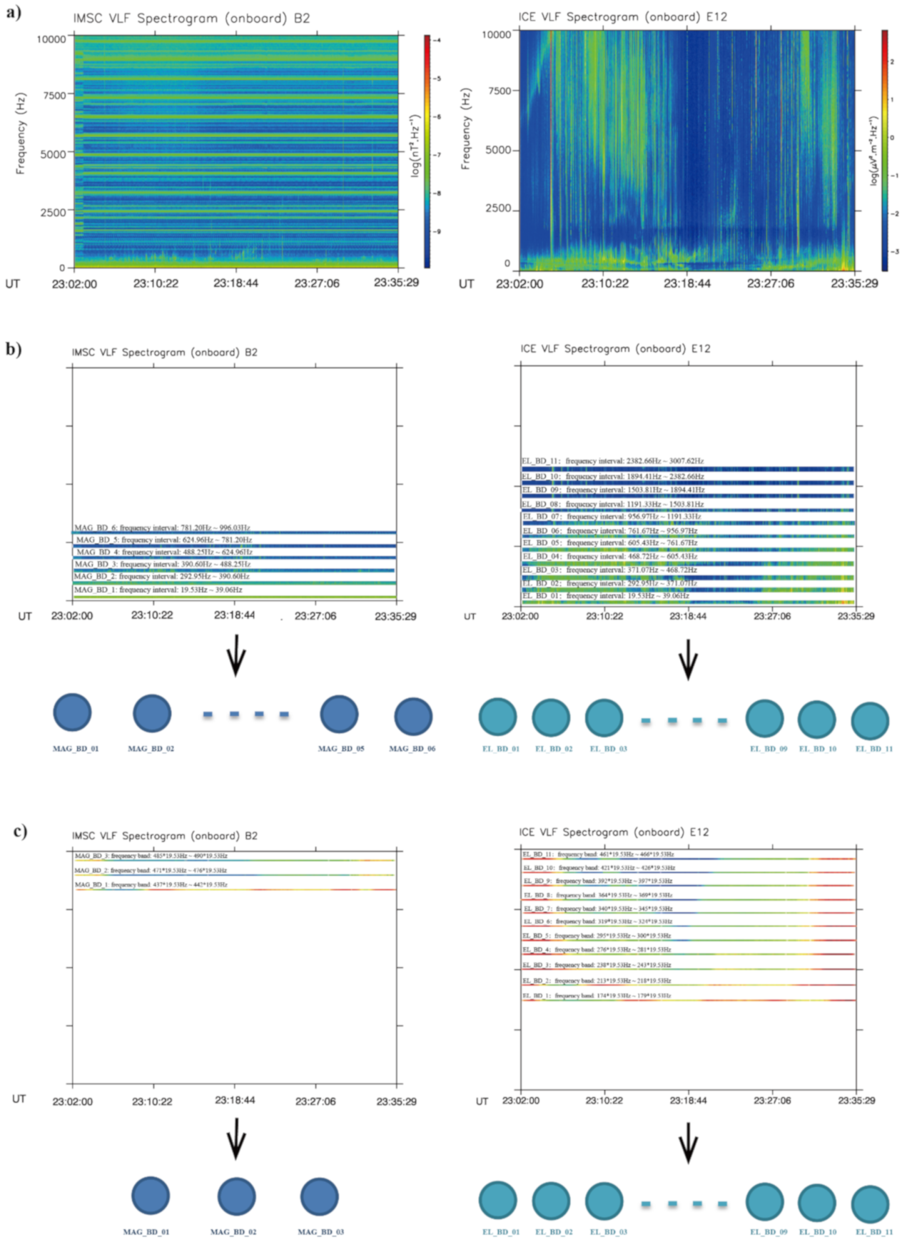
2.2. Data Preprocessing

We found that the power spectra of electric and magnetic fields are basically consistent temporally and spatially although they come from two different instruments. After the data integration, the initial data involve 27,347,148 records in total.

First of all, we carefully process the data. (1) We removed the 2004 data and conducted our analysis on the data starting from 2005. This is because magneto-torquers worked during 3 time intervals around a half-orbit at the beginning of the DEMETER mission (the interference can be seen with the IMSC), and at the same time, calibration signals must be prepared each time the mode is changing, i.e., from survey to burst or from burst to survey at the beginning of each half-orbit. Unfortunately, DEMETER encountered a magnetic storm at the beginning of November 2004, and the big Sumatra earthquake in December 2004 came with many aftershocks. (2) We removed the frequencies from 1 up to 8 kHz with the IMSC, as the IMSC has interference that spectrograms lines at constant frequencies, which is due to the onboard electronics and it is impossible to remove the interference. We removed the man-made waves from the ground-based Very Low Frequency (VLF) transmitters, i.e., waves with frequencies above 11.5 kHz (the three Russian ALPHA transmitters start around 12 kHz) with both the IMSC and ICE. (3) We identified and removed all the half-orbits where electronics were in trouble, mostly due to heavy particles or wrong telecommands. (4) We excluded the time intervals when troubles occurred in the electric data and the very spectacular events called structured emissions with turbulence and interference (SETI) [43]. (5) To avoid density perturbations due to magnetic activity [44], we restricted our analysis to the data with the Kp index of smaller than or equal to 3. After the data preprocessing, a total of 25,546,213 records were used for training.

2.3. Frequency Bands Logarithmically Spaced

Different from the approach presented by Němec et al. [21], which focuses on a wide frequency bandwidth, we focus on low frequencies in our study and select frequency bands logarithmically spaced in ULF and in ELF. In order to focus on the low frequencies, the frequency range in our analysis is limited to below 3 kHz with ICE and below 1 kHz with IMSC, respectively. We have separately selected 11 and 6 frequency bands for the electric and magnetic field, respectively (Figure 1b).

For power spectrum data of the electric field (ICE), we select 11 frequency bands logarithmically spaced and limited to below 3 kHz:

ELF (3 to 30 Hz): 1*19.53~2*19.53 Hz;

ULF(300 to 3000 Hz): 15*19.53~19*19.53 Hz, 19*19.53~24*19.53 Hz, 24*19.53~31*19.53 Hz, 31*19.53~39*19.53 Hz, 39*19.53~49*19.53 Hz, 49*19.53~61*19.53 Hz, 61*19.53~77*19.53 Hz, 77*19.53~97*19.53 Hz, 97*19.53~122*19.53 Hz and 122*19.53~154*19.53 Hz.

For power spectrum data of the magnetic field (IMSC), we select 6 frequency bands logarithmically spaced and limited to below 1 kHz:

ELF (3 to 30 Hz): 1*19.53~2*19.53 Hz;

ULF (300 to 1000 Hz): 15*19.53~20*19.53 Hz, 20*19.53~25*19.53 Hz, 25*19.53~32*19.53 Hz, 32*19.53~40*19.53 Hz and 40*19.53~51*19.53 Hz.

Then, we calculate the value for the frequency band according to the following formula:

$$spectra\_data={\log }_{10}\left({10}^{a_m}+ {10}^{a_{m+1}}\dots + {10}^{a_n}\right)$$

(1)

where a_m and a_n correspond to power spectrum data of the upper and lower bounds of the frequency band.

Finally, a total of 17 features (11 electric and 6 magnetic field frequency band measurements) are used as inputs to train the machine learning tools. The purpose of this is to exclude the interference of the spacecraft and cover the entire studied low-frequency range in ULF and ELF as uniformly as possible.

In this study, a total of 8760 earthquakes with magnitudes larger than or equal to 5.0 and depths less than or equal to 40 km occurred all over the world from January 2005 to December 2010 according to the USGS catalogue (http://neic.usgs.gov/). In order to avoid the mixed-effects pre-seismic and post-seismic activities, we excluded the values used more than once in the analysis since otherwise it is impossible to determine which earthquake the observed data can be attributed to. In order to verify the reliability and improve the robustness of the machine learning tools, we generate 8760 artificial non-seismic events and stagger the time and place to match when and where the real earthquakes occur. The artificial non-seismic events generation method we use here is to select a period of time and space so that the spatio-temporal range does not involve real earthquakes, and then generate an artificial non-seismic event by randomly sampling the time, latitude and longitude within the spatio-temporal range with the following constraints: (1) the time is not 10 days before and after a real earthquake occurrence time, (2) the longitude is not within 10° of the longitude of a real earthquake and (3) the latitude is not within 10° of the latitude of a real earthquake.

As reported by Němec et al. [21], a significant decrease in the wave intensity is observed several hours before earthquakes started. Given that there is no universal standard for the temporal window, we set the temporal window to be 48 h or 7 days before an earthquake hits for comparisons. The spatial feature is the distance away from the epicenter where the earthquake occurs. Again, since there is no agreed standard, the radius of the earthquake area that is expected to change is given by Dobrovolsky’s formula:

$${\mathrm{R} = 10}^{0.43M}$$

(2)

where R is the radius of the earthquake preparation zone in kilometers and M is the earthquake magnitude [45].

So, the circular region with its center at the epicenter and a radius given by the Dobrovolsky’s formula and a deviation of 10° were selected as the spatial features in our study (Figure 2).

Moreover, the day- and nighttime data were treated separately. After the data preprocessing was completed, datasets (

Table 1. Datasets are used as input to the models.

	Night/Daytime	Spatial Feature (with Its Center at the Epicenter and the Dobrovolsky Radius/a Deviation of 10°)	Temporal Feature	Frequency Feature	Artificial Non-Seismic Events/Data Generation
DataSet 01	Nighttime	the Dobrovolsky radius	48 h	low frequencies	stagger the time and place
DataSet 02	Nighttime	a deviation of 10°	7 days	low frequencies	stagger the time and place
DataSet 03	Daytime	the Dobrovolsky radius	48 h	low frequencies	stagger the time and place
DataSet 04	Daytime	a deviation of 10°	7 days	low frequencies	stagger the time and place
DataSet 05	Nighttime	the Dobrovolsky radius	48 h	high frequencies	stagger the time and place
DataSet 06	Nighttime	the Dobrovolsky radius	48 h	low frequencies	only stagger the time
DataSet 07	Nighttime	the Dobrovolsky radius	48 h	high frequencies	only stagger the time
DataSet 20	Nighttime	the Dobrovolsky radius	7 days	low frequencies	stagger the time and place
DataSet 21	Nighttime	the Dobrovolsky radius	10 days	low frequencies	stagger the time and place
DataSet 22	Nighttime	the Dobrovolsky radius	20 days	low frequencies	stagger the time and place
DataSet 23	Nighttime	the Dobrovolsky radius	30 days	low frequencies	stagger the time and place
DataSet I	Nighttime	the Dobrovolsky radius	48 h	low frequencies	10–20 days before/after real earthquakes
DataSet II	Nighttime	the Dobrovolsky radius	48 h	low frequencies	20–30 days before/after real earthquakes
DataSet III	Nighttime	the Dobrovolsky radius	48 h	low frequencies	30–40 days before/after real earthquakes
DataSet IV	Nighttime	the Dobrovolsky radius	48 h	low frequencies	40–50 days before/after real earthquakes
DataSet V	Nighttime	the Dobrovolsky radius	48 h	low frequencies	50–60 days before/after real earthquakes
DataSet VI	Nighttime	the Dobrovolsky radius	48 h	low frequencies	60–70 days before/after real earthquakes

) were generated and subsequently used as inputs to train the machine learning tools.

3. Methodology

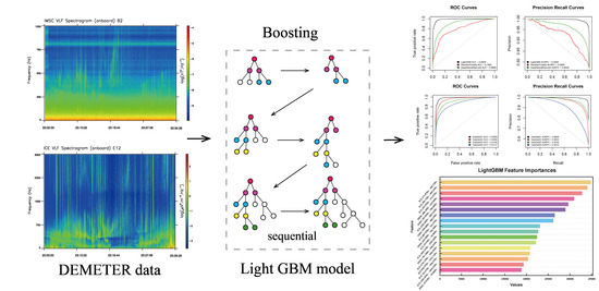
3.1. Overview of Our Methodology

The methodology carried out in this study is shown in a schematic way (Figure 3). After data preprocessing, each dataset was carefully split into two contiguous pieces: 90% for training models, which is from January 2005 to June 2010, and 10% for testing purposes and final evaluation, which is from June 2010 to December 2010. The top classifier is chosen by a quick assessment and model comparison of 15 different spot-checking algorithms along with the deep neural network (DNN) method. Bayesian optimization [46] and five-fold cross-validation [47] are used in this process for hyperparameter tuning and performance evaluation, respectively. In this way, we can perform model selection with high confidence, assuring that a robust model is selected and used. Moreover, the most important features of electromagnetic pre-earthquake perturbations can be obtained from the best classifier.

3.2. Machine Learning Methods

In this study, we formulate the perturbation discrimination task of pre-earthquake electromagnetism as a binary class classification problem, where the seismic-related data are labeled with 1 and non-seismic-related data are labeled with 0. Spot-checking algorithms are a quick assessment of a bunch of different algorithms on the problem so that you know which algorithms to focus on and which to discard [48]. As a classification problem in this study, we will try 15 spot-checking algorithms along with the DNN method on DataSet 01 with five-fold cross-validation, specifically: (1) linear algorithms: logistic regression [49], ridge regression [50], stochastic gradient descent classifier [51], passive aggressive classifier [52], linear discriminant analysis [53] and quadratic discriminant analysis [54]. (2) Nonlinear algorithms: classification and regression trees [55], extra tree [56], support vector machine [57] and naive Bayes [58]. (3) Ensemble algorithms: AdaBoost [59], random forest [60], gradient boosting machine [61], extreme gradient boosting [62] and light gradient boosting machine [63]. (4) Deep learning algorithms: deep neural network [64,65]. Benchmarking was performed on a server equipped with two Intel ^® Xeon ^® Processor E5-2650 v4 CPU, 128 GB of memory and NVIDIA Tesla V100 GPU.

Among these methods, LightGBM is a fast, distributed and high-performance gradient boosting framework based on ensembling tree-structured algorithms and has been widely used for ranking, classification and many other machine learning tasks [63]. After partitioning the training data onto a number of datasets, LightGBM performs both local and global voting in each iteration, and detailed explanations to this are documented in Meng et al. [66]. To investigate whether the frequency bands are seismic-related or not, the selected frequency bands are represented by feature vectors and encoded into the LightGBM-based classifier. LightGBM utilizes the histogram-based algorithm [67,68] to accelerate the training process, reduce memory consumption and optimize the parallel voting decision tree algorithm with advanced network communication. The training by LightGBM is usually much faster than many other algorithms such as support vector machines, therefore its name includes the word “Light”.

3.3. Bayesian Hyperparameter Tuning

Since the methods are sensitive to parameter selection, Bayesian hyperparameter tuning is used to choose the parameters that obtain the best performance. We use the negative of the area under the curve (AUC) as the return value (loss) of the objective function, and Bayesian optimization [46] selects the most promising hyperparameters that minimize an objective function by building the probability model based on past evaluation results of the objective. In this way, Bayesian optimization can achieve better performance on the test set while requiring fewer iterations than random and gird search. The search space of major parameters for LightGBM and DNN is provided in Table S1 and Table S3, respectively, and the maximum number of iterations for each model is set to 100. We use the Hyperopt python package [69] for the implementation of Bayesian optimization.

3.4. Five-Fold Cross-Validation

Cross-validation is a resampling procedure used to test how well the machine learning model performs. The classification results obtained in this study used five-fold cross-validation [70]. The overall dataset was divided into five subsets randomly. In each verification step, one subset was selected as a test set, while the remaining ones formed a training set. The model was trained on the training set and then verified by the test one. This process was repeated five times, and a different subset of samples was selected each time so that every subset was selected once in turn. The final was calculated according to averages of the five subsets.

3.5. Performance Evaluation

After we have determined the parameters for each method, the performance of each method based on these parameters was compared with the others. We use five performance measures, namely accuracy, sensitivity, specificity, the AUC and the area under the recall–precision curve (AURPC), to evaluate the performance of each method.

AUC is the area under the receiver operating characteristic (ROC) curve, which is a plot of true positive rate (TPR) against false positive rate (FPR). AURPC is also used in our work to evaluate the performance, which is regarded as a good alternative to AUC [71].

The accuracy (ACC) is defined as

$$ACC=\frac{TP+TN}{TP+TN+FP+FN}$$

(3)

The sensitivity (TPR) is defined as

$$TPR=\frac{TP}{TP+FN}$$

(4)

The specificity (TNR) is defined as

$$TNR=\frac{TN}{TN+FP}$$

(5)

where TP is the number of true positives (a true positive test result is one that detects the condition when the condition is present), TN is the number of true negatives (a true negative test result is one that does not detect the condition when the condition is absent), FP is the number of false positives (a false positive test result is one that detects the condition when the condition is absent) and FN is the number of false negatives (a false negative test result is one that does not detect the condition when the condition is present).

3.6. Feature Importance

The importance of a feature is computed as the (normalized) reduction in the errors brought by that feature. It is also known as the Gini importance. The single node importance NI is defined as

$$\begin{array}{c}NI=Gini\left(\left\{Nod{e}_{split}\right\},\left\{w\right\}\right)-Gini\left(\left\{Nod{e}_{left}\right\},\left\{w_{left}\right\}\right)\\ -Gini\left(\left\{Nod{e}_{right}\right\},\left\{w_{right}\right\}\right)\end{array}$$

(6)

where $Nod{e}_{split}$ is the split non-leaf node in the decision tree, $Nod{e}_{right}$ and $Nod{e}_{left}$ are the right and left children nodes of $Nod{e}_{split}$ and $w$ is the sample weight.

The importance of each feature on a decision tree is then calculated as

$$feature importance= \frac{1}{M}{\displaystyle \sum }_m^M\frac{{{\displaystyle \sum }}_f^{F}N{I}_f^{\left(m\right)}}{{{\displaystyle \sum }}_k^{K}N{I}_k^{\left(m\right)}}$$

(7)

So, M is the number of the trees in LightGBM, F is the number of non-leaf nodes which employ the target feature to split data and K is the total number of non-leaf in the m-th tree.

4. Results and Discussion

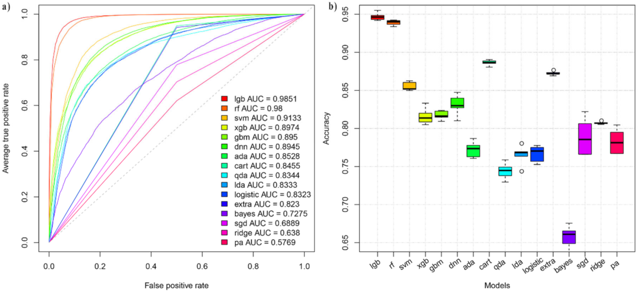
4.1. Evaluation of the Model Performance

As shown in Figure 3, all the benchmarking methods were used to construct models for classification, based on DataSet 01 with the generated features. Figure 4 shows histograms and summary statistics of the seismic and non-seismic input sample data, which show the values of the frequency band (ICE: from 19.53 to 39.06 Hz), where the percentage corresponds to the count of each bin divided by the sum of counts of all bins. From Figures S1 and S2, no significant imbalance was found in the positive (there was an earthquake) and negative (there was no earthquake) cases in all input data, suggesting the credibility and stability of the machine learning models. The data were preprocessed with normalization or not and with standardization or not, i.e., we have four cases, before we feed the data into the machine learning tool [72], which are important parameters in the Bayesian optimization process. The performance of each of the compared methods was summarized using the specificity, sensitivity, accuracy, precision and AUC measures on the training dataset of DataSet 01 (

Table 2. Performance comparison between 15 spot-checking algorithms along with the deep neural network (DNN)method on the training dataset of DataSet 01.

Method	DataSet 01
	Specificity	Sensitivity	Accuracy	Precision	AUC
lgb	0.941	0.948	0.947	0.981	0.985
rf	0.909	0.948	0.939	0.971	0.98
svm	0.833	0.861	0.855	0.944	0.913
xgb	0.821	0.814	0.816	0.937	0.897
gbm	0.813	0.818	0.817	0.935	0.895
dnn	0.812	0.836	0.830	0.936	0.894
ada	0.786	0.767	0.772	0.922	0.852
cart	0.768	0.922	0.886	0.929	0.845
qda	0.829	0.718	0.744	0.933	0.834
lda	0.771	0.763	0.764	0.916	0.833
logistic	0.771	0.765	0.766	0.916	0.832
extra	0.730	0.915	0.872	0.918	0.823
bayes	0.685	0.648	0.657	0.872	0.727
sgd	0.611	0.766	0.730	0.879	0.688
ridge	0.321	0.954	0.807	0.822	0.638
pa	0.363	0.789	0.690	0.833	0.576

). In particular, for the sake of the comparison, we plotted the ROC curves [73] (Figure 5a) and the boxplot curves of accuracy (Figure 5b) to show the performance of each method. We adopt the ROC (receiver operating characteristic) curve as a performance metric, which depicts relative trade-offs between true positive (benefits) and false positive (costs). Besides, we show AUC (area under the ROC curve) as an indicator of the distinguishing power of different models. Higher AUC conduces to a preferable method for the prediction task. By analogy, higher AUC leads to a better method to distinguish between seismic and non-seismic electromagnetic data.

From Figure 5 and Table 2, the average AUC of each spot-checking algorithm ranges from 0.576 to 0.98 and the average accuracy of each method ranges from 0.657 to 0.939. We found that the light gradient boosting machine (LightGBM) was the top classifier both from the ROC curves (Figure 5a) and boxplot curves of accuracy (Figure 5b), and was also the best method from the evaluation metrics (Table 2). We have also noticed random forest (RF) generated good performance almost as well as LightGBM for DataSet 01, with the exception of specificity which is slightly lower. To investigate further, we also compared LightGBM with RF using the other four benchmarking datasets (Table 1). In general, as shown in

Table 3. Performance comparison between LightGBM and random forest on a training dataset of DataSet 02, DataSet 03, DataSet 04 and DataSet 05.

Method	DataSet 02
	Specificity	Sensitivity	Accuracy	Precision	AUC
LightGBM	0.870	0.874	0.872	0.880	0.945
Random Forest	0.855	0.879	0.868	0.869	0.942
Method	DataSet 03
	Specificity	Sensitivity	Accuracy	Precision	AUC
LightGBM	0.870	0.811	0.834	0.955	0.916
Random Forest	0.832	0.833	0.832	0.944	0.910
Method	DataSet 04
	Specificity	Sensitivity	Accuracy	Precision	AUC
LightGBM	0.836	0.752	0.789	0.851	0.869
Random Forest	0.832	0.747	0.785	0.847	0.865
Method	DataSet 05
	Specificity	Sensitivity	Accuracy	Precision	AUC
LightGBM	0.656	0.725	0.719	0.875	0.757
Random Forest	0.631	0.738	0.713	0.869	0.747

, we discover that almost all performance metrics of LightGBM are slightly higher than that of RF in all the datasets presented in Table 1, which means that the LightGBM method is more accurate than RF in discriminating electromagnetic pre-earthquake perturbations. We also compared LightGBM with RF using AUC. From Figure 6, we can see that the AUC curve of LightGBM is also a little higher than that of RF in all the datasets, implying that LightGBM outperformed RF, and this could be explained by the fact that the hyperparameters in LightGBM, e.g., the number of trees, depth and the learning rate, are tunable, but this is not possible for RF. DNN was applied to DataSet 01 and generated the accuracy of 0.830 and AUC of 0.894. Compared to DNN, the accuracy of LightGBM increases to 0.947, and DNN finds its AUC worse than that of LightGBM on DataSet 01 (Table 2). We have also explored different DNN networks (e.g., with different layers such as 7, 8, 9 and 10; increased number of the iterations to 180 (which was 100)) (Table S3, Supplemental Dataset S2) and have not found one that works better than LightGBM (the sheet with the name of DNN in DataSet S2 shows that the best AUC is 0.8957, which is only slightly better than the result of the relatively small search space, which is with the AUC of 0.894, whilst the AUC of LightGBM is 0.986). Although DNN is constructed with three fully connected layers, its performance is worse than that of LightGBM. This might be because deep learning architectures require significantly large training sets (a large number of earthquakes) for system optimization, which are not available in the current research because of the very limited resources.

Moreover, to investigate if there is a bias in the LightGBM model, a random labels test was performed. Practically, based on DataSet 01, we generated a set of elements with random labels, i.e., the labels are “wrong”, and named the dataset Dataset 08. The figures in Figure 7 indicate that the LightGBM model is not able to learn on the “wrong” dataset, which means the LightGBM model passed the level 0 test. The AUCs of LightGBM on DataSet 01 and DataSet 08 are 0.985 and 0.507 (

Table 4. Performance comparison between thirteen datasets on the method LightGBM.

Dataset	LightGBM
	Specificity	Sensitivity	Accuracy	Precision	AUC	AURPC
DataSet 01	0.887	0.980	0.959	0.967	0.986	0.995
DataSet 02	0.895	0.893	0.894	0.907	0.960	0.965
DataSet 03	0.862	0.835	0.841	0.954	0.919	0.974
DataSet 04	0.848	0.743	0.79	0.856	0.873	0.903
DataSet 05	0.638	0.760	0.732	0.877	0.768	0.910
DataSet 06	0.848	0.717	0.782	0.826	0.863	0.872
DataSet 07	0.904	0.411	0.657	0.811	0.684	0.733
DataSet 08	0.788	0.246	0.370	0.798	0.507	0.775
DataSet I	0.819	0.811	0.815	0.818	0.891	0.896
DataSet II	0.852	0.784	0.818	0.842	0.894	0.898
DataSet III	0.833	0.807	0.820	0.829	0.896	0.902
DataSet IV	0.828	0.811	0.820	0.826	0.896	0.899
DataSet V	0.852	0.759	0.805	0.837	0.887	0.890
DataSet VI	0.827	0.785	0.806	0.821	0.891	0.898

), respectively, and the accuracies on DataSet 01 and DataSet 08 are 0.950 and 0.370 (Table 4), respectively.

Furthermore, as seen in Table 4 and Figure 8, all four benchmarking datasets were used to compare the results of using different spatial and temporal features by LightGBM. In this comparison, we employed both AUC and AURPC to evaluate the performance by using our five-fold cross-validation (benchmarking) dataset. In general, we discover that the datasets with the nighttime (DataSets 01 and 02 in Table 4) lead to better classification performance than the datasets with the daytime (DataSets 03 and 04 in Table 4) for the same different spatial and temporal features, respectively (Table 1 and Table 4). The ROC and recall-precision curves of LightGBM for all the datasets are shown in Figure 8 for performance comparison. The daytime data show no significant difference, probably because the ionospheric conditions are generally more disturbed and then the detection of seismo-electromagnetic effects becomes difficult. This result is in good alignment with the statistical results of electromagnetic perturbations connected to seismic activities [21,22,23,24].

4.2. Considering Different Spatial Windows

We also observed that LightGBM performed better in the circular region with its center at the epicenter and a radius given by the Dobrovolsky’s formula (DataSets 01 and 03 in Table 4) than in the circular region with its center at the epicenter and a radius given by a deviation of 10° (DataSets 02 and 04 in Table 4), with AUC improved from 0.985/0.919 to 0.960/0.873. Geometrically, the disturbance propagating upwards from the ground surface can change the properties of the ionosphere, and the radius of the affected area is in good alignment with the results calculated by the earthquake magnitude and Dobrovolsky’s formula.

In order to further prove that “data within a circular region with its center at the epicenter and its radius given by the Dobrovolsky’s formula and the time window of about a few hours before shocks” are more useful in discriminating electromagnetic pre-earthquake perturbations, satellite datasets of the spatial window with its center at the epicenter and a deviation of 3° (DataSet 09), 5° (DataSet 10), 7° (DataSet 11) and 12° (DataSet 12) have been generated (

Table 5. Datasets with different features used as input to the models.

	Night/Daytime	Spatial Feature	Temporal Feature	Earthquake Magnitude/Number of Earthquakes	Number of Data Used for Training
DataSet 09	Nighttime	with its center at the epicenter and a deviation of 3°	48 h	all/8760	444,772
DataSet 10	Nighttime	with its center at the epicenter and a deviation of 5°	48 h	all/8760	1,243,216
DataSet 11	Nighttime	with its center at the epicenter and a deviation of 7°	48 h	all/8760	2,360,36
DataSet 12	Nighttime	with its center at the epicenter and a deviation of 12°	48 h	all/8760	6,517,967
DataSet 13	Nighttime	with its center at the epicenter and the Dobrovolsky radius	48 h	5.0~5.5/6818	110,839
DataSet 14	Nighttime	with its center at the epicenter and the Dobrovolsky radius	48 h	5.5~6.0/1813	63,584
DataSet 15	Nighttime	with its center at the epicenter and the Dobrovolsky radius	48 h	above 6.0/589	176,945
DataSet 16	Nighttime	with its center at the epicenter and the Dobrovolsky radius	48 h	1:2	176,943
DataSet 17	Nighttime	with its center at the epicenter and the Dobrovolsky radius	48 h	1:3	462,642
DataSet 18	Nighttime	with its center at the epicenter and the Dobrovolsky radius	48 h	1:4	535,777
DataSet 19	Nighttime	with its center at the epicenter and the Dobrovolsky radius	48 h	1:5	603,208

).

Figure 9 provides the recall-precision and ROC curves of the five datasets (including DataSet 01) with different spatial windows.

Table 6. Further performance comparison between datasets on the method LightGBM.

	Testing Set								Training Set
	AUC	AURPC	FP	FN	Specificity	Precision	Sensitivity	Accuracy	Accuracy
DataSet 01	0.986	0.995	90	54	0.887	0.967	0.980	0.959	1.000
DataSet 09	0.929	0.941	286	358	0.865	0.873	0.846	0.855	0.995
DataSet 10	0.923	0.939	724	1170	0.873	0.885	0.826	0.848	0.985
DataSet 11	0.911	0.931	1502	2455	0.861	0.873	0.808	0.832	0.962
DataSet 12	0.881	0.910	4657	8559	0.837	0.858	0.766	0.797	0.943
DataSet 13	0.919	0.913	69	109	0.883	0.856	0.790	0.839	1.000
DataSet 14	0.952	0.984	29	32	0.803	0.940	0.935	0.904	1.000
DataSet 15	0.959	0.998	33	12	0.484	0.981	0.993	0.975	1.000
DataSet 16	0.940	0.998	27	9	0.460	0.984	0.995	0.980	1.000
DataSet 17	0.924	0.937	330	377	0.845	0.865	0.849	0.847	1.000
DataSet 18	0.925	0.926	332	469	0.882	0.862	0.816	0.851	1.000
DataSet 19	0.923	0.904	322	566	0.907	0.861	0.780	0.853	1.000
DataSet 20	0.916	0.971	1003	512	0.619	0.888	0.939	0.864	1
DataSet 21	0.907	0.967	922	1574	0.758	0.918	0.868	0.841	0.967
DataSet 22	0.903	0.967	1549	3463	0.780	0.926	0.849	0.832	0.938
DataSet 23	0.899	0.964	1994	5618	0.809	0.930	0.826	0.822	0.909

presents the classification performance with the five datasets of different spatial windows using LightGBM. From Table 6, the AUC on each dataset ranges from 0.881 to 0.986 and the average accuracy ranges from 0.797 to 0.959. It remains true that by increasing the distance of the spatial window, the performance of AUC and accuracy decreases by about 0.084 and 0.027, respectively. Based on these results, we conclude that the choice of the spatial window size is influencing, to a certain extent, the performance of the LightGBM model. Although the LightGBM model is capable of discriminating electromagnetic pre-earthquake perturbations with different spatial window sizes, it gives the best performance on the dataset with its center at the epicenter and its radius given by the Dobrovolsky’s formula and the time window of about 48 h before shocks.

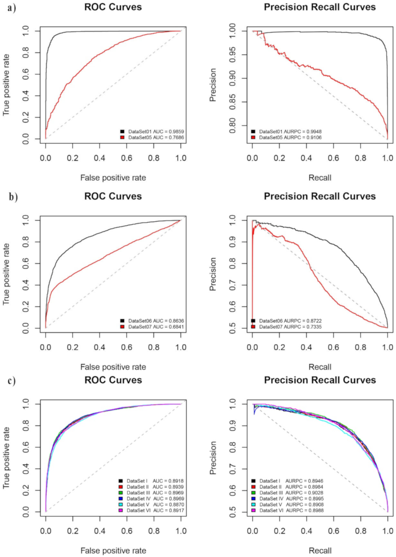
4.3. Considering Different Frequency Bands

To study the influences of different frequency bands on discriminating electromagnetic pre-earthquake perturbations, the frequency range of the analysis is limited to 3–10 kHz with ICE and 8–10 kHz with IMSC (high frequencies), and the approach to select frequency bands is the same as Němec et al. [21]. We have separately selected 11 and 3 frequency bands for the electric and magnetic fields, respectively (Figure 1c), which form the new dataset (DataSet 05). For power spectrum data of the electric field (ICE), we select 11 frequency bands logarithmically spaced and limited to 3–10 kHz (174*19.53~179*19.53 Hz, 213*19.53~218*19.53 Hz, 238*19.53~243*19.53 Hz, 276*19.53~281*19.53 Hz, 295*19.53~300*19.53 Hz, 319*19.53~324*19.53 Hz, 340*19.53~345*19.53 Hz, 364*19.53~369*19.53 Hz, 392*19.53~397*19.53 Hz, 421*19.53~426*19.53 Hz and 461*19.53~466*19.53 Hz). For power spectrum data of the magnetic field (IMSC), we select three frequency bands logarithmically spaced and limited to 8–10 kHz (437*19.53~442*19.53 Hz, 471*19.53~476*19.53 Hz and 485*19.53~490*19.53 Hz).

As illustrated in Table 4, DataSet 01 (the data with the frequency feature below 3 kHz with ICE and below 1 kHz with IMSC) and DataSet 05 (the data with the frequency feature at 3–10 kHz with ICE and 8–10 kHz with IMSC) were used for discriminating electromagnetic pre-earthquake perturbations. We discover that DataSet 01 shows better classification performance than DataSet 05 for the LightGBM classifier: The AUCs of LightGBM on DataSets 01 and 05 are 0.985 and 0.768, respectively, and the accuracies on DataSets 01 and 05 are 0.950 and 0.732, respectively. From this observation, we conclude that the datasets with low frequencies (below 3 kHz with ICE and below 1 kHz with IMSC) enable the electromagnetic pre-earthquake perturbations discrimination to achieve better accuracy than those with high frequencies. The ROC and recall-precision curves of the LightGBM model on DataSets 01 and 05 are shown in Figure 10a for performance comparison.

4.4. Considering the Earthquake Geographical Region

As the above method for generating artificial non-seismic events would step too far away from the earthquake geographical region, in order to further verify the reliability of the machine learning models, we refine the method by selecting “the same regions” but focusing “outside time windows” of real earthquakes. Practically, for each of the real earthquakes, we select earthquake-related data using the two constraints: “time inside a 20-day time window (ten days before/after earthquakes)” and “distance inside the Dobrovolsky’s radius”, then we select all data named A which are seismic-related data based on the real earthquakes. Then, we select data named B using only one constraint, “distance is inside the Dobrovolsky’s radius” from real earthquakes. By excluding A from B, we get C, which is apparently a non-seismic-related dataset, but inside the same earthquakes geographical region. Then, we can select the seismic-related data to form A and non-seismic-related data from C. After the data preprocessing is completed, DataSet 06 (the data with the frequency feature below 3 kHz with ICE and below 1 kHz with IMSC) and DataSet 07 (the data with the frequency feature at 3–10 kHz with ICE and 8–10 kHz with IMSC) are generated (Table 1) and are used as inputs to train the machine learning models. Performance comparison between the two datasets on the LightGBM method is illustrated in Table 4. The ROC and recall-precision curves of the LightGBM method on DataSet 06 and DataSet 07 are shown in Figure 10b. From Table 4 and Figure 10b, it could be noticed that the AUCs of LightGBM on DataSet 06 and DataSet 07 are 0.863 and 0.684, respectively, and the accuracies on DataSet 06 and DataSet 07 are 0.782 and 0.657, respectively. The LightGBM method provides better classification performance on DataSet 06 than on DataSet 07. In summary, although we use a new method to select the seismic-related data and non-seismic-related data, our work shows that the datasets with low frequency make it easier to discriminate the electromagnetic pre-earthquake perturbations, i.e., the data selection method has little (if not no) effect on the results.

To further explore the possible reason for the results mentioned above, we consider a new method for non-seismic-related data selection using a certain time window with a fixed width (ten days). Practically, for each of the real earthquakes, we select earthquake-related data using the three constraints: “time inside a 20-day time window (ten days before/after earthquakes)”, “distance within the Dobrovolsky’s radius” and “frequency feature below 3 kHz with ICE and below 1 kHz with IMSC”, and we name the selected data D. Besides, we select another version of data named E similarly as we select D except that the first constraint is changed to “time inside a 40-day time window (twenty days before/after earthquakes)”. We select another version of data named F by excluding D from E, i.e., the data in F is inside a time window with a fixed width (10–20 days before/after earthquakes). We then augment the seismic-related data all these non-seismic data and obtain a dataset called DataSet I. Similarly, we obtain DataSet II (20–30 days before/after earthquakes), DataSet III (30–40 days before/after earthquakes), DataSet IV (40–50 days before/after earthquakes), DataSet V (50–60 days before/after earthquakes) and DataSet VI (60–70 days before/after earthquakes) (Table 1). The last six rows of Table 4 illustrate LightGBM’s performance on the six datasets and Figure 10c shows the ROC and recall-precision curves of the LightGBM method on the six datasets. As is shown by Table 4 and Figure 10c, the method has similar performance on the six datasets, e.g., the AUCs of LightGBM on all six datasets are around 0.89 and the accuracies are around 0.81, i.e., LightGBM performs worse than on DataSet 01 since on DataSet 01 the AUC is 0.985 and its accuracy is 0.950. It remains true that by remaining on the same geographical location in simulating the non-seismic data, the performances decrease by about 0.09 of AUC and 0.14 of accuracy. That is, by simulating the non-seismic data in the vicinity of the faults (earthquake geographical region), the results of the LightGBM performance are worse than if you simulate the non-seismic data far from the faults. Based on these results, we conclude that the choice of the geographical region used to simulate the training set of non-seismic data is influencing, to a certain extent, the performance of the LightGBM model, by reducing its capability in discriminating electromagnetic pre-earthquake perturbations.

4.5. Considering the Earthquake Mangitude

Earthquake magnitude may play an active role on pre-earthquake perturbations identification. To demonstrate the influence of magnitudes, we have divided the earthquakes into groups of three, which are 6818 earthquakes with magnitudes between 5.0 and 5.5, 1813 earthquakes with magnitudes between 5.5 and 6.0 and 589 earthquakes with magnitudes of 6 and over, and the corresponding datasets are DataSet 13, DataSet 14 and DataSet 15 (Table 5).

Table 6 illustrates the LightGBM method’s performance on the four datasets (including DataSet 01). As is shown in Table 5, the method has similar performance over the four datasets, e.g., the AUC of the LightGBM method on all four datasets is around 0.96 (ranging from 0.919 to 0.986), and the accuracy is around 0.93 (ranging from 0.839 to 0.8975). Figure 11 shows the recall-precision and ROC curves displaying the performance of LightGBM on the datasets; we also observe a similar tendency in the performance of our method on the three datasets, which suggests that the LightGBM model provides satisfactory performance on discriminating electromagnetic pre-earthquake perturbations on the datasets with different magnitudes. Moreover, it can be concluded from Table 6 that the larger the magnitude, the better the classification performance. This is also in line with the reality.

Although the datasets are quite different, these results indicate that the LightGBM model can be used to produce reliable predictions using the datasets with different magnitudes and provide good performance.

4.6. Considering an Unbalanced Dataset

As the actual earthquake problem is always highly unbalanced, where non-earthquakes instances are always higher as compared to earthquakes. In order to provide a realistic performance overview, we try our proposed method on an unbalanced dataset in this section. To investigate whether or not our proposed method is capable of predicting an earthquake with unbalanced datasets, datasets with the positive to negative ratio of 1:2 (DataSet 16), 1:3 (DataSet 17), 1:4 (DataSet 18) and 1:5 (DataSet 19) have been generated (shown in Table 5).

Table 6 illustrates the proposed method’s performance on the five datasets (including DataSet 01). As shown in Figure 12, the method has similar performance on the five datasets, e.g., the PR AUCs of the proposed method on all five datasets are around 0.96 (ranges from 0.904 to 0.998) and the ROC AUCs are around 0.96 (ranges from 0.923 to 0.986). Figure 12 shows the ROC and recall-precision curves, and we also observe a similar tendency in the performance of our method on the five datasets, suggesting that our method provides a good performance for pre-earthquake perturbations discrimination on the unbalanced datasets. Despite that the five unbalanced datasets are different, these results indicate that our method is less sensitive to the positive to negative ratio, and that our method can be used to identify electromagnetic pre-earthquake perturbations using unbalanced datasets, that is, it can provide a good realistic performance.

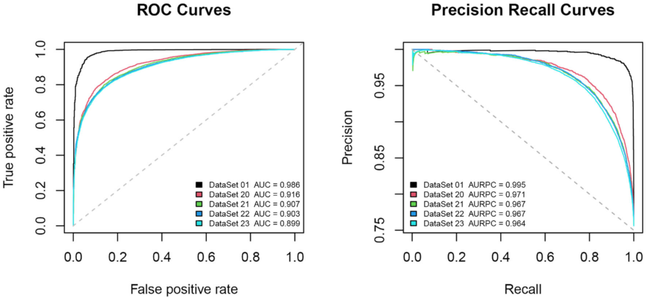
4.7. Considering Different Temporal Windows

We have observed that the dataset with a temporal window of 48 h (DataSet 01) has good classification performance. In order to investigate whether or not the LightGBM method is capable of identifying electromagnetic pre-earthquake perturbations with different temporal windows, datasets with temporal windows of 7 days (DataSet 20), 10 days (DataSet 21), 20 days (DataSet 22) and 30 days (DataSet 23) have been generated (shown in Table 1).

Figure 13 provides the ROC and recall-precision curves of the five datasets with different temporal windows. Table 6 presents the classification performance with different temporal windows using LightGBM. From Table 6, the AUC ranges from 0.899 to 0.986 and the AURPC ranges from 0.964 to 0.995 on different datasets. It remains true that by increasing the days of the temporal window, the performances decrease by about 0.087 for AUC and 0.031 for AURPC. That is, the LightGBM model’s performance is worse than if we increase the days of the temporal window. Based on these results, we conclude that the choice of the temporal window size is influencing, to a certain extent, the performance of the LightGBM model, by reducing its capability in identifying pre-earthquake perturbations. Regarding the machine learning methods, the LightGBM method performed better on the smaller dataset. This is due to the nature of trees, i.e., inherently fewer samples could train a better tree structure and produce better performance. Although the LightGBM model is capable of identifying perturbations with different temporal window sizes, it gives the best performance on the dataset with our initial selection of the temporal window of 48 h.

4.8. Dominant Features from LightGBM

In comparison with the blind features-based DNN model, LightGBM allows the importance of features to be determined during classification, i.e., the importance of each element in distinguishing one class from another. Gini importance is utilized to measure the importance of a feature and calculated as the sum of the split scores (across all trees) containing the feature, proportional to the number of samples it splits [63]. As shown in Figure 14, the frequency interval from 371.07 to 468.72 Hz of ICE, the frequency interval from 468.72 to 605.43 Hz of ICE, the frequency interval from 292.95 to 371.07 Hz of ICE, the frequency interval from 488.25 to 624.96 Hz of IMSC and the frequency interval from 292.95 to 390.60 Hz of IMSC are the most important features for the LightGBM model. A machine learning method trained using earthquake and non-earthquake electromagnetic data can demonstrate how the electromagnetic data have been influenced by the earthquake process.

The above results are well illustrated in Figure 15 and Figure 16, which show perturbations observed in the electric and magnetic field near the epicenter of some earthquakes in low frequency. Figure 15 presents perturbations three days before the Indonesian earthquake occurred on 17 July 2006 with a magnitude of 7.7, and the data related to the orbits were very close to the epicenter (9.28° S, 107.38° E). Perturbations are observed in the electric and magnetic fields near the epicenter in the form of intensification with the cutoff frequency in the range of about 350–400 Hz in ELF, as indicated by the arrow, reported by Bhattacharya et al. [74]. From Figure 16, perturbations are observed five days before the earthquake occurred on 30 August 2005 18:10:45 UT with a magnitude of 6.2, where the epicenter of the quake is 38.55° north latitude and 143.06° east longitude, and similar perturbations are observable with intensification at around 500 Hz in ELF in both the electric field and magnetic field. In addition, some examples of earthquake precursors for VLF temporary variations are demonstrated by Eppelbaum and Finkelstein [75].

Figure 17a shows the histograms and summary statistics obtained for distances from the epicenters of the seismic-related data. It can be seen that the distances interval from 100 to 200 km is observed as a key feature. The time interval from 10 to 11 h before the time of the main shock has the largest weight (Figure 17b).

4.9. Discussion

We summarize the previous studies using machine learning for pre-earthquake perturbation analysis for the DEMETER data, shown in

Table 7. Previous studies using machine learning for pre-earthquake perturbations analysis from the DEMETER data. BPNN: back-propagation neural network. MARBDP: mining association rule based on dynamic pruning. DTW: dynamic time warping. S4VMs: safe semi-supervised support vector machines. IAP: plasma analyzer instrument. ISL: Langmuir probes instrument.

Study	Study Area	Study Period	Input Data	Model	Objective and Performance
Xu et al. [77]	The globe	2007–2008	Ne, Te, Ti, NO+, H+ and He+ from IAP and ISL	BPNN	predict seismic events in 2008. Accuracy: 69.96%.
Li and Parrot [33]	The globe	June 2004–December 2010	Total ion density (the sum of H+, He+ and O+)) from IAP	Statistics model	statistics of data perturbation. Sensitivity: 65.25% Specificity: 71.95%
Wang, Pi, Zhang and Shen [76]	Taiwan, China	January 2008–June 2008	Ne, Ni, Te, Ti, NO+, H+, He+ and O+ from IAP and ISL	MARBDP	predict earthquakes of Ms >5.0 from January 2008 to June 2008. sensitivity: 70.01%
Zang et al. [78]	The globe	June 2004–December 2010	Ne, Ni, Te, Ti, NO+, H+, He+ and O+ from IAP and ISL	calculate asymmetry and stability using DTW distance	recognizing epicenter-neighboring orbits during strong seismic Sensitivity: 65.03%
Zang et al. [79]	The globe	June 2004–December 2010	Ne, Te, Ti, O+, plasma potential	S4VMs with kernel combination	seismic classification-based method for recognizing epicenter-neighboring orbit. Sensitivity: 79.36% Specificity: 98.34%
Our proposed method	The globe	June 2004–December 2010	Low-frequency power spectra from IMSC and ICE	LightGBM	discriminate electromagnetic pre-earthquake perturbations Sensitivity: 95.41% Specificity: 93.69% Accuracy: 95.01%

. Through the performance comparison among these studies, the result shows that among those popular machine learning methods, the LightGBM method outperforms the others, i.e., it gives the best performance on all the benchmarking datasets.

Compared with the existing studies on pre-earthquake perturbation analysis, this study has three main advantages. First, hyperparametric optimization and cross-validation are used in all the engaged methods, which allows us to find the best parameters for these methods. In this way, we can perform technology selection with high confidence, assuring that a robust method is selected and used. Second, differing from the traditional statistics and data mining methods, a more advanced machine learning architecture is used for pre-earthquake perturbation analysis. Last, most of the existing methods are validated by a small number of samples, such as Wang et al. [76], which may have a strong bias toward the values in a larger area or a longer time interval. However, LightGBM is applied to different datasets, whereas global features are learned during the training process. Hence, LightGBM has a strong generalization ability.

The hiss of the ionosphere at low altitude with the frequency between 100 Hz and 1 kHz can propagate along the magnetic field and penetrate into the topside ionosphere [80,81,82,83,84]. In our study, the frequency intervals from 371.07 to 468.72 Hz of ICE, 468.72 to 605.43 Hz of ICE, 292.95 to 371.07 Hz of ICE, 488.25 to 624.96 Hz of IMSC and 292.95 to 390.60 Hz of IMSC are the most important features rendered by LightGBM when we discriminate the earthquake and non-earthquake electromagnetic data. Our results suggest that sudden changes in the cutoff frequency of the ELF hiss or observation of whistlers near to the epicenter of earthquakes can help to discriminate earthquake-related electromagnetic data. Due to the existence of such phenomena before earthquakes, they could be regarded as short-term precursors to earthquakes.

5. Conclusions

We have explored 15 spot-checking classification algorithms along with the deep neural network model on the classification problem, and the top classifier based on a variety of combined features generated by low-frequency power spectra of the electric and magnetic fields was used to improve the performance of electromagnetic pre-earthquake perturbations discrimination from the DEMETER data. Our work shows that the LightGBM model outperforms the other models including DNN.

In our paper, the selection of temporal and spatial windows was used both during training and the testing process. In addition, for clearer presentation, we have provided Table S4 which summarizes the main variables and results for all datasets. From Table S4, we could observe that electromagnetic pre-earthquake data in the circular region with its center at the epicenter and a radius given by the Dobrovolsky’s formula and a few hours before the times of the shocks are more reasonable in discriminating electromagnetic pre-earthquake perturbations, and the classification model also performs better on those with the nighttime than the datasets with the daytime; the results also show that the earthquake geographical region reduces the machine learning model’s capability in discriminating electromagnetic pre-earthquake perturbations. Moreover, the distance interval from 100 to 200 km from the epicenter and the time interval from 10 to 11 h before the main shock are the key features from the results of the histograms and summary statistics.

Observations of dominant features of electromagnetic pre-earthquake perturbations are derived from LightGBM, and the observations along with the study results of the influences of different frequency band ranges on discriminating electromagnetic pre-earthquake perturbations support that we can discriminate earthquake-related electromagnetic data using low-frequency signals. The physical explanations about this could consider the lithosphere–atmosphere–ionosphere coupling [85,86,87,88,89], which showed that the effect of seismic crustal stress enables mechanical energy to be transformed to heat energy, and then transmitted to the earth surface through pores in rocks. At the same time, the local stress enhancement and the occurrence of micro-earthquakes can cause numerous micro-cracks and micro-fractures inside the lithosphere, so that the geo gases and fluids within the lithosphere, such as H2 and Rn, would spill out along these channels. The increase in geo gases in the atmosphere stimulates physical processes and chemical reactions from the ground surface up to the ionosphere, which can also produce an additional electric field, penetrate into the ionosphere and cause a large-scale ionosphere perturbation, and finally cause electromagnetic pre-earthquake perturbations.

Overall, our results show that machine learning is a promising tool for processing high-dimensional electromagnetic pre-earthquake perturbations data and that it supports investigations of seismic development.

References

1. Shen, X.H.; Zhang, X.M.; Hong, S.Y.; Jing, F.; Zhao, S.F. Progress and development on multi-parameters remote sensing application in earthquake monitoring in China. Earthq. Sci. 2013, 26, 427–437. [Google Scholar] [CrossRef] [Green Version]
2. Parrot, M. First results of the DEMETER micro-satellite. Planet. Space Sci. 2006, 54, 411–558. [Google Scholar] [CrossRef]
3. Parrot, M.; Berthelier, J.J.; Lebreton, J.P.; Sauvaud, J.A.; Santolik, O.; Blecki, J. Examples of unusual ionospheric observations made by the DEMETER satellite over seismic regions. Phys. Chem. Earth Parts A/B/C 2006, 31, 486–495. [Google Scholar] [CrossRef]
4. Zhang, X.; Shen, X.; Liu, J.; Ouyang, X.; Qian, J.; Zhao, S. Analysis of ionospheric plasma perturbations before Wenchuan earthquake. Nat. Hazards Earth Syst. Sci. 2009, 9, 1259–1266. [Google Scholar] [CrossRef] [Green Version]
5. Błeçki, J.; Parrot, M.; Wronowski, R. Studies of the electromagnetic field variations in ELF frequency range registered by DEMETER over the Sichuan region prior to the 12 May 2008 earthquake. Int. J. Remote Sens. 2010, 31, 3615–3629. [Google Scholar] [CrossRef]
6. Sarkar, S.; Gwal, A.K. Satellite monitoring of anomalous effects in the ionosphere related to the great Wenchuan earthquake of May 12, 2008. Nat. Hazards 2010, 55, 321–332. [Google Scholar] [CrossRef]
7. Ryu, K.; Parrot, M.; Kim, S.G.; Jeong, K.S.; Chae, J.S.; Pulinets, S.; Oyama, K.I. Suspected seismo-ionospheric coupling observed by satellite measurements and GPS TEC related to the M7.9 Wenchuan earthquake of 12 May 2008. J. Geophys. Res. Space Phys. 2014, 119, 10305–10323. [Google Scholar] [CrossRef] [Green Version]
8. Liu, J.Y.; Chen, Y.I.; Huang, C.C.; Parrot, M.; Shen, X.H.; Pulinets, S.A.; Yang, Q.S.; Ho, Y.Y. A spatial analysis on seismo-ionospheric anomalies observed by DEMETER during the 2008 M8.0 Wenchuan earthquake. J. Asian Earth Sci. 2015, 114, 414–419. [Google Scholar] [CrossRef]
9. Walker, S.N.; Kadirkamanathan, V.; Pokhotelov, O.A. Changes in the ultra-low frequency wave field during the precursor phase to the Sichuan earthquake: DEMETER observations. Ann. Geophys. 2013, 31, 1597–1603. [Google Scholar] [CrossRef] [Green Version]
10. Píša, D.; Parrot, M.; Santolík, O. Ionospheric density variations recorded before the 2010 Mw 8.8 earthquake in Chile. J. Geophys. Res. Space Phys. 2011, 116. [Google Scholar] [CrossRef] [Green Version]
11. Zhang, X.; Qian, J.; Ouyang, X.; Shen, X.; Cai, J.; Zhao, S. Ionospheric electromagnetic perturbations observed on DEMETER satellite before Chile M7.9 earthquake. Earthq. Sci. 2009, 22, 251–255. [Google Scholar] [CrossRef] [Green Version]
12. Ho, Y.Y.; Liu, J.Y.; Parrot, M.; Pinçon, J.L. Temporal and spatial analyses on seismo-electric anomalies associated with the 27 February 2010 M=8.8 Chile earthquake observed by DEMETER satellite. Nat. Hazards Earth Syst. Sci. 2013, 13, 3281–3289. [Google Scholar] [CrossRef] [Green Version]
13. Ho, Y.Y.; Jhuang, H.K.; Su, Y.C.; Liu, J.Y. Seismo-ionospheric anomalies in total electron content of the GIM and electron density of DEMETER before the 27 February 2010 M8.8 Chile earthquake. Adv. Space Res. 2013, 51, 2309–2315. [Google Scholar] [CrossRef]
14. Louerguioui, S.; Gaci, S.; Zaourar, N. Irregularities of the ionospheric plasma and the ULF electric components obtained from DEMETER satellite experiments above Chile earthquake (27 February 2010). Arab. J. Geosci. 2014, 8, 2433–2441. [Google Scholar] [CrossRef] [Green Version]
15. Mofiz, U.A.; Battiston, R. Possible ion-acoustic soliton formation in the ionospheric perturbations observed on DEMETER before the 2007 Pu’er earthquake. Earthq. Sci. 2009, 22, 257–262. [Google Scholar] [CrossRef] [Green Version]
16. He, Y.; Yang, D.; Qian, J.; Parrot, M. Anomaly of the ionospheric electron density close to earthquakes: Case studies of Pu’er and Wenchuan earthquakes. Earthq. Sci. 2011, 24, 549–555. [Google Scholar] [CrossRef] [Green Version]
17. Shen, X.H.; Zhang, X.; Liu, J.; Zhao, S.F.; Yuan, G.P. Analysis of the enhanced negative correlation between electron density and electron temperature related to earthquakes. Ann. Geophys. 2015, 33, 471–479. [Google Scholar] [CrossRef] [Green Version]
18. Stangl, G.; Boudjada, M.Y.; Biagi, P.F.; Krauss, S.; Maier, A.; Schwingenschuh, K.; Al-Haddad, E.; Parrot, M.; Voller, W. Investigation of TEC and VLF space measurements associated to L’Aquila (Italy) earthquakes. Nat. Hazards Earth Syst. Sci. 2011, 11, 1019–1024. [Google Scholar] [CrossRef] [Green Version]
19. Bertello, I.; Piersanti, M.; Candidi, M.; Diego, P.; Ubertini, P. Electromagnetic field observations by the DEMETER satellite in connection with the 2009 L’Aquila earthquake. Ann. Geophys. 2018, 36, 1483–1493. [Google Scholar] [CrossRef] [Green Version]
20. Athanasiou, M.A.; Anagnostopoulos, G.C.; Iliopoulos, A.C.; Pavlos, G.P.; David, C.N. Enhanced ULF radiation observed by DEMETER two months around the strong 2010 Haiti earthquake. Nat. Hazards Earth Syst. Sci. 2011, 11, 1091–1098. [Google Scholar] [CrossRef]
21. Němec, F.; Santolík, O.; Parrot, M.; Berthelier, J.J. Spacecraft observations of electromagnetic perturbations connected with seismic activity. Geophys. Res. Lett. 2008, 35. [Google Scholar] [CrossRef] [Green Version]
22. Němec, F.; Santolík, O.; Parrot, M. Decrease of intensity of ELF/VLF waves observed in the upper ionosphere close to earthquakes: A statistical study. J. Geophys. Res. Space Phys. 2009, 114. [Google Scholar] [CrossRef]
23. Píša, D.; Němec, F.; Parrot, M.; Santolík, O. Attenuation of electromagnetic waves at the frequency ~1.7 kHz in the upper ionosphere observed by the DEMETER satellite in the vicinity of earthquakes. Ann. Geophys. 2012, 55. [Google Scholar] [CrossRef]
24. Píša, D.; Němec, F.; Santolík, O.; Parrot, M.; Rycroft, M. Additional attenuation of natural VLF electromagnetic waves observed by the DEMETER spacecraft resulting from preseismic activity. J. Geophys. Res. Space Phys. 2013, 118, 5286–5295. [Google Scholar] [CrossRef] [Green Version]
25. Hobara, Y.; Nakamura, R.; Suzuki, M.; Hayakawa, M.; Parrot, M. Ionospheric perturbations observed by the low altitude satellite DEMETER and possible relation with seismicity. J. Atmos. Electr. 2013, 33, 21–29. [Google Scholar] [CrossRef] [Green Version]
26. Ryu, K.; Lee, E.; Chae, J.S.; Parrot, M.; Pulinets, S. Seismo-ionospheric coupling appearing as equatorial electron density enhancements observed via DEMETER electron density measurements. J. Geophys. Res. Space Phys. 2014, 119, 8524–8542. [Google Scholar] [CrossRef] [Green Version]
27. He, Y.; Yang, D.; Zhu, R.; Qian, J.; Parrot, M. Variations of electron density and temperature in ionosphere based on the DEMETER ISL data. Earthq. Sci. 2010, 23, 349–355. [Google Scholar] [CrossRef] [Green Version]
28. He, Y.; Yang, D.; Qian, J.; Parrot, M. Response of the ionospheric electron density to different types of seismic events. Nat. Hazards Earth Syst. Sci. 2011, 11, 2173–2180. [Google Scholar] [CrossRef] [Green Version]
29. Yan, R.; Parrot, M.; Pinçon, J.-L. Statistical Study on Variations of the Ionospheric Ion Density Observed by DEMETER and Related to Seismic Activities. J. Geophys. Res. Space Phys. 2017, 122, 412–421. [Google Scholar] [CrossRef] [Green Version]
30. Parrot, M. Statistical analysis of the ion density measured by the satellite DEMETER in relation with the seismic activity. Earthq. Sci. 2011, 24, 513–521. [Google Scholar] [CrossRef] [Green Version]
31. Li, M.; Parrot, M. “Real time analysis” of the ion density measured by the satellite DEMETER in relation with the seismic activity. Nat. Hazards Earth Syst. Sci. 2012, 12, 2957–2963. [Google Scholar] [CrossRef] [Green Version]
32. Parrot, M. Statistical analysis of automatically detected ion density variations recorded by DEMETER and their relation to seismic activity. Ann. Geophys. 2012, 55. [Google Scholar] [CrossRef]
33. Li, M.; Parrot, M. Statistical analysis of an ionospheric parameter as a base for earthquake prediction. J. Geophys. Res. Space Phys. 2013, 118, 3731–3739. [Google Scholar] [CrossRef] [Green Version]
34. Parrot, M.; Li, M. Statistical analysis of the ionospheric density recorded by the demeter satellite during seismic activity. Pre-Earthq. Process. 2018. [Google Scholar] [CrossRef]
35. Zhang, J.; Liu, P.; Zhang, F.; Song, Q. CloudNet: Ground-based cloud classification with deep convolutional neural network. Geophys. Res. Lett. 2018. [Google Scholar] [CrossRef]
36. Bergen, K.J.; Johnson, P.A.; de Hoop, M.V.; Beroza, G.C. Machine learning for data-driven discovery in solid Earth geoscience. Science 2019, 363. [Google Scholar] [CrossRef] [PubMed]
37. Rouet-Leduc, B.; Hulbert, C.; Johnson, P.A. Continuous chatter of the Cascadia subduction zone revealed by machine learning. Nat. Geosci. 2018, 12, 75–79. [Google Scholar] [CrossRef]
38. Hulbert, C.; Rouet-Leduc, B.; Johnson, P.A.; Ren, C.X.; Rivière, J.; Bolton, D.C.; Marone, C. Similarity of fast and slow earthquakes illuminated by machine learning. Nat. Geosci. 2018, 12, 69–74. [Google Scholar] [CrossRef]
39. Perol, T.; Gharbi, M.; Denolle, M. Convolutional neural network for earthquake detection and location. Sci. Adv. 2018, 4, e1700578. [Google Scholar] [CrossRef] [Green Version]
40. Yoon, C.E.; O’Reilly, O.; Bergen, K.J.; Beroza, G.C. Earthquake detection through computationally efficient similarity search. Sci. Adv. 2015, 1, e1501057. [Google Scholar] [CrossRef] [PubMed] [Green Version]
41. Berthelier, J.J.; Godefroy, M.; Leblanc, F.; Malingre, M.; Menvielle, M.; Lagoutte, D.; Brochot, J.Y.; Colin, F.; Elie, F.; Legendre, C.; et al. ICE, the electric field experiment on DEMETER. Planet. Space Sci. 2006, 54, 456–471. [Google Scholar] [CrossRef]
42. Parrot, M.; Benoist, D.; Berthelier, J.J.; Błęcki, J.; Chapuis, Y.; Colin, F.; Elie, F.; Fergeau, P.; Lagoutte, D.; Lefeuvre, F.; et al. The magnetic field experiment IMSC and its data processing onboard DEMETER: Scientific objectives, description and first results. Planet. Space Sci. 2006, 54, 441–455. [Google Scholar] [CrossRef]
43. Parrot, M.; Berthelier, J.J.; Blecki, J.; Brochot, J.Y.; Hobara, Y.; Lagoutte, D.; Lebreton, J.P.; Němec, F.; Onishi, T.; Pinçon, J.L.; et al. Unexpected very low frequency (VLF) radio events recorded by the ionospheric satellite DEMETER. Surv. Geophys. 2015, 36, 483–511. [Google Scholar] [CrossRef]
44. Parrot, M.; Buzzi, A.; Santolík, O.; Berthelier, J.J.; Sauvaud, J.A.; Lebreton, J.P. New observations of electromagnetic harmonic ELF emissions in the ionosphere by the DEMETER satellite during large magnetic storms. J. Geophys. Res. 2006, 111. [Google Scholar] [CrossRef] [Green Version]
45. Dobrovolsky, I.; Zubkov, S.; Miachkin, V. Estimation of the size of earthquake preparation zones. Pure Appl. Geophys. 1979, 117, 1025–1044. [Google Scholar] [CrossRef]
46. Snoek, J.; Larochelle, H.; Adams, R.P. Practical bayesian optimization of machine learning algorithms. In Advances in Neural Information Processing Systems; Curran Associates Inc.: Lake Tahoe, NV, USA, 2012; pp. 2951–2959. [Google Scholar]
47. Rodriguez, J.D.; Perez, A.; Lozano, J.A. Sensitivity analysis of k-fold cross validation in prediction error estimation. IEEE Trans. Pattern Anal. Mach. Intell. 2009, 32, 569–575. [Google Scholar] [CrossRef] [PubMed]
48. Michie, D.; Spiegelhalter, D.J.; Taylor, C.C.; Campbell, J. (Eds.) Machine Learning, Neural and Statistical Classification; Ellis Horwood: Upper Saddle River, NJ, USA, 1994; p. 289. [Google Scholar]
49. Cox, D.R. The regression analysis of binary sequences. J. R. Stat. Soc. Ser. B 1958, 20, 215–232. [Google Scholar] [CrossRef]
50. Gruber, M. Improving Efficiency by Shrinkage: The James–Stein and Ridge Regression Estimators; Routledge: New York, NY, USA, 2017. [Google Scholar]
51. Bottou, L. Stochastic gradient descent tricks. In Neural Networks: Tricks of the Trade; Springer: Berlin/Heidelberg, Germany, 2012; pp. 421–436. [Google Scholar]
52. Crammer, K.; Dekel, O.; Keshet, J.; Shalev-Shwartz, S.; Singer, Y. Online passive-aggressive algorithms. J. Mach. Learn. Res. 2006, 7, 551–585. [Google Scholar]
53. Fisher, R.A. The Use of Multiple Measurements in Taxonomic Problems. Ann. Eugen. 1936, 7, 179–188. [Google Scholar] [CrossRef]
54. Friedman, J.; Hastie, T.; Tibshirani, R. The Elements of Statistical Learning; Springer Series in Statistics New York: New York, NY, USA, 2001; Volume 1. [Google Scholar]
55. Breiman, L. Classification and Regression Trees; Routledge: New York, NY, USA, 2017. [Google Scholar]
56. Geurts, P.; Ernst, D.; Wehenkel, L. Extremely randomized trees. Mach. Learn. 2006, 63, 3–42. [Google Scholar] [CrossRef] [Green Version]
57. Cortes, C.; Vapnik, V. Support-vector networks. Mach. Learn. 1995, 20, 273–297. [Google Scholar] [CrossRef]
58. Maron, M.E. Automatic indexing: An experimental inquiry. J. ACM 1961, 8, 404–417. [Google Scholar] [CrossRef]
59. Kégl, B. The return of AdaBoost. MH: Multi-class Hamming trees. arXiv 2013, arXiv:1312.6086. [Google Scholar]
60. Breiman, L. Random forests. Mach. Learn. 2001, 45, 5–32. [Google Scholar] [CrossRef] [Green Version]
61. Friedman, J.H. Greedy function approximation: A gradient boosting machine. Ann. Stat. 2001, 29, 1189–1232. [Google Scholar] [CrossRef]
62. Chen, T.; Guestrin, C. XGBoost: A scalable tree boosting system. In Proceedings of the 22nd ACM SIGKDD International Conference on Knowledge Discovery and Data Mining, San Francisco, CA, USA, 13–17 August 2016; pp. 785–794. [Google Scholar]
63. Ke, G.; Meng, Q.; Finley, T.; Wang, T.; Chen, W.; Ma, W.; Ye, Q.; Liu, T.-Y. LightGBM: A highly efficient gradient boosting decision tree. In Proceedings of the 31st International Conference on Neural Information Processing Systems, Long Beach, CA, USA, 4–9 December 2017; pp. 3149–3157. [Google Scholar]
64. Goodfellow, I.; Bengio, Y.; Courville, A. Deep Learning; MIT Press: Cambridge, MA, USA, 2016. [Google Scholar]
65. LeCun, Y.; Bengio, Y.; Hinton, G. Deep learning. Nature 2015, 521, 436–444. [Google Scholar] [CrossRef]
66. Meng, Q.; Ke, G.; Wang, T.; Chen, W.; Ye, Q.; Ma, Z.-M.; Liu, T.-Y. A communication-efficient parallel algorithm for decision tree. In Proceedings of the 30th International Conference on Neural Information Processing Systems, Barcelona, Spain, 5–10 December 2016; pp. 1279–1287. [Google Scholar]
67. Ranka, S.; Singh, V. CLOUDS: A decision tree classifier for large datasets. In Proceedings of the 4th Knowledge Discovery and Data Mining Conference, New York, NY, USA, 27–31 August 1998; pp. 2–8. [Google Scholar]
68. Jin, R.; Agrawal, G. Communication and memory efficient parallel decision tree construction. In Proceedings of the 2003 SIAM International Conference on Data Mining, San Francisco, CA, USA, 1–3 May 2003; pp. 119–129. [Google Scholar]
69. Bergstra, J.; Yamins, D.; Cox, D.D. Making a science of model search: Hyperparameter optimization in hundreds of dimensions for vision architectures. In Proceedings of the 30th International Conference on International Conference on Machine Learning—Volume 28, Atlanta, GA, USA, 16–21 June 2013; pp. I-115–I-123. [Google Scholar]
70. Kohavi, R. A study of cross-validation and bootstrap for accuracy estimation and model selection. In Proceedings of the 14th International Joint Conference on Artificial Intelligence, Montreal, QC, Canada, 20–25 August 1995; pp. 1137–1145. [Google Scholar]
71. Davis, J.; Goadrich, M. The relationship between Precision-Recall and ROC curves. In Proceedings of the 23rd International Conference on Machine Learning, Pittsburgh, PA, USA, 25–29 June 2006; pp. 233–240. [Google Scholar]
72. Iwata, S. Weights and measures in the indus valley. In ENCYCLOPAEDIA of the History of Science, Technology, and Medicine in Non-Western Cultures, 2nd ed.; Selin, H., Ed.; Springer: Berlin/Heidelberg, Germany, 2008; pp. 2254–2255. [Google Scholar]
73. Sing, T.; Sander, O.; Beerenwinkel, N.; Lengauer, T.J.B. ROCR: Visualizing classifier performance in R. Bioinformatics 2005, 21, 3940–3941. [Google Scholar] [CrossRef]
74. Bhattacharya, S.; Sarkar, S.; Gwal, A.K.; Parrot, M. Electric and magnetic field perturbations recorded by DEMETER satellite before seismic events of the 17th July 2006 M 7.7 earthquake in Indonesia. J. Asian Earth Sci. 2009, 34, 634–644. [Google Scholar] [CrossRef]
75. Eppelbaum, L.; Finkelstein, M. Radon Emanation, Magnetic and VLF Temporary Variations: Removing Components not Associated with Dynamic Processes. 1998. Available online: https://www.researchgate.net/publication/231817102_Radon_emanation_magnetic_and_VLF_temporary_variations_removing_components_not_associated_with_dynamic_processes (accessed on 4 November 2020).
76. Wang, Y.D.; Pi, D.C.; Zhang, X.M.; Shen, X.H. Seismo-ionospheric precursory anomalies detection from DEMETER satellite data based on data mining. Nat. Hazards 2014, 76, 823–837. [Google Scholar] [CrossRef]
77. Xu, F.; Song, X.; Wang, X.; Su, J. Neural network model for earthquake prediction using DMETER data and seismic belt information. In Proceedings of the 2010 Second WRI Global Congress on Intelligent Systems, Wuhan, China, 16–17 December 2010; pp. 180–183. [Google Scholar]
78. Zang, S.; Pi, D.; Zhang, X.; Shen, X. Recognizing methods for epicenter-neighboring orbits with ionospheric information from DEMETER satellite data. Adv. Space Res. 2017, 60, 980–990. [Google Scholar] [CrossRef]
79. Zang, S.; Pi, D.; Zhang, X.; Shen, X. Seismic classification-based method for recognizing epicenter-neighboring orbits. Adv. Space Res. 2017, 59, 1886–1894. [Google Scholar] [CrossRef]
80. Santolík, O.; Parrot, M. Case studies on the wave propagation and polarization of ELF emissions observed by Freja around the local proton gyrofrequency. J. Geophys. Res. Space Phys. 1999, 104, 2459–2475. [Google Scholar] [CrossRef]
81. Santolík, O.; Parrot, M. Application of wave distribution function methods to an ELF hiss event at high latitudes. J. Geophys. Res. Space Phys. 2000, 105, 18885–18894. [Google Scholar] [CrossRef]
82. Santolík, O.; Chum, J.; Parrot, M.; Gurnett, D.; Pickett, J.; Cornilleau-Wehrlin, N. Propagation of whistler mode chorus to low altitudes: Spacecraft observations of structured ELF hiss. J. Geophys. Res. Space Phys. 2006, 111. [Google Scholar] [CrossRef] [Green Version]
83. Chen, L.; Santolík, O.; Hajoš, M.; Zheng, L.; Zhima, Z.; Heelis, R.; Hanzelka, M.; Horne, R.B.; Parrot, M. Source of the low-altitude hiss in the ionosphere. Geophys. Res. Lett. 2017, 44, 2060–2069. [Google Scholar] [CrossRef] [Green Version]
84. Xia, Z.; Chen, L.; Zhima, Z.; Santolík, O.; Horne, R.B.; Parrot, M. Statistical characteristics of ionospheric hiss waves. Geophys. Res. Lett. 2019, 46, 7147–7156. [Google Scholar] [CrossRef] [Green Version]
85. Pulinets, S.A.; Morozova, L.I.; Yudin, I.A. Synchronization of atmospheric indicators at the last stage of earthquake preparation cycle. Res. Geophys. 2015, 4. [Google Scholar] [CrossRef] [Green Version]
86. Pulinets, S.; Davidenko, D. Ionospheric precursors of earthquakes and Global Electric Circuit. Adv. Space Res. 2014, 53, 709–723. [Google Scholar] [CrossRef]
87. Kuo, C.L.; Lee, L.C.; Huba, J.D. An improved coupling model for the lithosphere-atmosphere-ionosphere system. J. Geophys. Res. Space Phys. 2014, 119, 3189–3205. [Google Scholar] [CrossRef]
88. Harrison, R.G.; Aplin, K.L.; Rycroft, M.J. Atmospheric electricity coupling between earthquake regions and the ionosphere. J. Atmos. Sol.-Terr. Phys. 2010, 72, 376–381. [Google Scholar] [CrossRef] [Green Version]
89. Pulinets, S.; Ouzounov, D. Lithosphere–Atmosphere–Ionosphere Coupling (LAIC) modelAn unified concept for earthquake precursors validation. J. Asian Earth Sci. 2011, 41, 371–382. [Google Scholar] [CrossRef]
Figure 1. (a) Original power spectra of electric field (right pane) and magnetic field (left pane), the frequency range of our analysis is limited to below 10 kHz. (b) Processing to 11 and 6 frequency bands for the electric and magnetic field, respectively, the frequency range is limited to below 3 kHz with instrument champ electrique (ICE) and below 1kHz with instrument magnetic search coil (IMSC). (c) Processing to 11 and 3 frequency bands for the electric field (3–10 kHz) and magnetic field (8–10 kHz), respectively.
Remotesensing 12 03643 g001
Figure 2. Schematic diagrams showing data points on-orbit (orange dots), at the earthquake epicenter (red stars) and at the areas around the epicenters (dashed circles), which are considered for selecting seismic-related data. The radii of the circles are not at the scale of diagrams.
Remotesensing 12 03643 g002
Figure 3. The flowchart of the proposed machine learning framework.
Remotesensing 12 03643 g003
Figure 4. (a) Histograms and summary statistics of the seismic and (b) non-seismic input sample data. The figure shows the values of each frequency band (displays numerical data by grouping data into “bins” of equal width), and the percentage is that of the counts of each bin divided by the sum of counts of all bins.
Remotesensing 12 03643 g004
Figure 5. (a) Receiver operating characteristic (ROC) curves of 16 spot-checking algorithms displaying the performance on nighttime with its center at the epicenter and a radius given by the Dobrovolsky’s formula and 48 h before an earthquake (training dataset of Dataset 01). (b) Boxplot curves of accuracy with 16 spot-checking algorithms displaying the performance on Dataset 01. Note that the light gradient boosting machine is referred to as lgb in the figure, the other 15 algorithms are abbreviated as: logistic—logistic regression, ridge—ridge regression, sgd—stochastic gradient descent, pa—passive aggressive, lda—linear discriminant analysis, qda—quadratic discriminant analysis, cart—classification and regression trees, xgb—extreme gradient boosting, extra—extra tree, svm—support vector machine, bayes—naive Bayes, ada—AdaBoost, rf—random forest, gbm—gradient boosting machine, dnn—deep neural network.
Remotesensing 12 03643 g005
Figure 6. ROC curves displaying the performance comparison between LightGBM (lgb) and random forest (rf) on a training dataset of DataSet 01.
Remotesensing 12 03643 g006
Figure 7. Recall-precision and ROC curves displaying the performance of LightGBM on testing datasets of DataSet 01 and DataSet 08.
Remotesensing 12 03643 g007
Figure 8. Recall-precision and ROC curves displaying the performance of LightGBM on testing datasets of Dataset 01, DataSet 02, DataSet 03 and DataSet 04. Note that the scale of values on the vertical axis is different from recall-precision curves (0.5–1.) and ROC curves (0.–1.).
Remotesensing 12 03643 g008
Figure 9. Recall-precision and ROC curves displaying the performance of LightGBM on testing datasets of Dataset 01, DataSet 09, DataSet 10, DataSet 11 and DataSet 12.
Remotesensing 12 03643 g009
Figure 10. Recall-precision and ROC curves displaying the performance of LightGBM on testing datasets of (a) DataSet 01 and DataSet 05, and (b) DataSet 06 and DataSet 07 and (c) from DataSet I to DataSet VI. Note that the scale of values on the vertical axis is different from recall-precision curves (0.5–1.) and ROC curves (0.–1.).
Remotesensing 12 03643 g010
Figure 11. Recall-precision and ROC curves displaying the performance of LightGBM on testing datasets of DataSet 01, DataSet 13, DataSet 14 and DataSet 15. Note that the scale of values on the vertical axis is different from recall-precision curves (0.5–1.) and ROC curves (0.–1.).
Remotesensing 12 03643 g011
Figure 12. Recall-precision and ROC curves displaying the performance of LightGBM on testing datasets of DataSet 01, DataSet 16, DataSet 17, DataSet 18 and DataSet 19. Note that the scale of values on the vertical axis is different from recall-precision curves (0.5–1.) and ROC curves (0.–1.).
Remotesensing 12 03643 g012
Figure 13. Recall-precision and ROC curves displaying the performance of LightGBM on testing datasets of DataSet 01, DataSet 20, DataSet 21, DataSet 22 and DataSet 23. Note that the scale of values on the vertical axis is different from recall-precision curves (0.75–1.) and ROC curves (0.–1.).
Remotesensing 12 03643 g013
Figure 14. The features’ importance given by LightGBM model on Dataset 01. The larger the value, the more important a feature.
Remotesensing 12 03643 g014
Figure 15. Electric and magnetic field spectrogram for 14 July 2006 (orbit 10,821 downward). From top to bottom, the first panel shows the results of the electric field spectrogram up to 1 kHz, and the second one displays the magnetic results up to 1 kHz, where perturbations are highlighted by the red arrow.
Remotesensing 12 03643 g015
Figure 16. Electric and magnetic field spectrogram for 25 August 2005 (orbit 06,091 downward). From top to bottom, the first panel shows the results of the electric field spectrogram up to 1.5 kHz, and the second one displays the magnetic results up to 1.5 kHz, where perturbations are highlighted by the red arrow.
Remotesensing 12 03643 g016
Figure 17. (a) The histograms and summary statistics obtained for distances from the epicenter of the seismic-related data. (b) The histograms and summary statistics obtained for time interval before the time of the earthquake. The percentage is that of the counts of each bin divided by the sum of counts of all bins.
Remotesensing 12 03643 g017