Detecting and Tracking Moving Airplanes from Space Based on Normalized Frame Difference Labeling and Improved Similarity Measures

Abstract

The emerging satellite videos provide the opportunity to detect moving objects and track their trajectories, which were not possible for remotely sensed imagery with limited temporal resolution. So far, most studies using satellite video data have been concentrated on traffic monitoring through detecting and tracking moving cars, whereas the studies on other moving objects such as airplanes are limited. In this paper, an integrated method for monitoring moving airplanes from a satellite video is proposed. First, we design a normalized frame difference labeling (NFDL) algorithm to detect moving airplanes, which adopts a non-recursive strategy to deliver stable detection throughout the whole video. Second, the template matching (TM) technique is utilized for tracking the detected moving airplanes in the frame sequence by improved similarity measures (ISMs) with better rotation invariance and model drift suppression ability. Template matching with improved similarity measures (TM-ISMs) is further implemented to handle the leave-the-scene problem. The developed method is tested on a satellite video to detect and track eleven moving airplanes. Our NFDL algorithm successfully detects all the moving airplanes with the highest F₁ score of 0.88 among existing algorithms. The performance of TM-ISMs is compared with both its traditional counterparts and other state-of-the-art tracking algorithms. The experimental results show that TM-ISMs can handle both rotation and leave-the-scene problems. Moreover, TM-ISMs achieve a very high tracking accuracy of 0.921 and the highest tracking speed of 470.62 frames per second.

1. Introduction

In the last decade, new satellite sensors capable of capturing videos have been developed and launched [1,2,3,4,5,6,7,8,9,10,11,12]. Unlike satellite images, the temporal resolution of a satellite video is determined by its frame rate. For example, the sensors onboard SkySat satellites can film panchromatic videos with a frame rate of 30 frames per second (fps) at one-meter spatial resolution [13], which means the sensors’ temporal resolution is approximately 0.03 s. Satellite videography offers a new perspective for earth observation and enables important applications such as moving object detection and tracking, which may not be fully achievable using traditional satellite images.

Moving object detection and tracking has been a hot topic in the remote sensing community [14,15,16,17]. Traditional studies utilized very high spatial resolution satellite images to monitor moving objects by taking advantage of the time gap between different sensors on the same satellite [14,16]. Due to the short time lag (e.g., only 0.2 s for Quickbird satellites), very limited dynamic information can be provided. In contrast, satellite video data possess a much longer duration of up to 90 s, which enables continuous detection and tracking of moving objects in a long period of time. A successful application of satellite video data is traffic monitoring, which can be achieved by a standard two-step procedure [4,7,12]. First, the locations of moving cars are extracted by a moving object detection algorithm. Second, detected cars are tracked in the frame sequence to estimate their motion properties, such as speeds and trajectories.

Using satellite video data to detect moving objects may encounter similar challenges as ordinary videos [18], such as foreground aperture, camouflage, and parallax motion. Although existing algorithms can address such problems with various adaptive models [1,3,10], stable detection may not be achieved for the early stage of the video [19]. Ideally, moving object detection and tracking algorithms should be integrated into a unified method so that the outcomes of detection can automatically provide the initial locations of moving objects immediately for tracking. However, most studies in remote sensing utilize standalone tracking algorithms with the initial locations of moving objects being manually defined [2,5,6,8,9,20]. Moreover, the concentration of most tracking algorithms is on suppressing model drift, which happens when the tracked location of an object deviates from the correct one. However, their performance under more complex conditions, such as rotation and leave-the-scene, has not been fully tested.

While attention in satellite videography has been given primarily to cars, airplanes have not been treated in much detail due to limited data availability. Encouragingly, more and more video satellites are being launched recently. Chang Guang Satellite Technology Co., Ltd, the vendor of Jilin-1 satellite video data, aims to establish a constellation of 138 satellites that achieves a 10-minute revisit capability for any location on earth. With increased data availability, satellite videography possesses great potential for the aviation industry in the foreseeable future. Satellite videography can monitor areas that cannot be covered by air search radars due to the curvature of the earth. Moreover, satellite videography can be used to capture stealth aircraft designed to be invisible for air search radars because the stealth of an aircraft is achieved by its surface coating, which can absorb radar waves but cannot absorb visible light waves.

In this study, we have developed an integrated method for detecting and tracking moving airplanes in a satellite video. The method consists of two algorithms: First, an algorithm named normalized frame differencing labeling (NFDL) is designed to provide stable detection throughout the satellite video. Second, the detected moving airplanes are tracked by template matching (TM) in the frame sequence. In this stage, improved similarity measures (ISMs) are devised to achieve both better rotation invariance and model drift suppression. This paper is structured as follows. In Section 2, we introduce the research background of satellite videography on moving object detection and tracking. The experimental data and proposed method are presented in Section 3. The experimental results for detecting and tracking eleven airplanes are reported in Section 4 and then discussed in Section 5. Finally, Section 6 concludes this paper.

2. Background

2.1. Moving Object Detection Algorithms

In the context of moving object detection, pixels of moving objects are called the foreground, and pixels of stationary objects, as well as unwanted moving objects, are called the background. Detecting moving objects in each video frame is conducted by subtracting background pixels from the whole video frame [21,22]. Based on Cheung and Kamath [23], background subtraction algorithms can be grouped into non-recursive and recursive algorithms. A non-recursive algorithm uses a series of previous video frames to estimate the temporal variation of each pixel, and a pixel significantly deviating from the estimated variation is considered as foreground [23]. Using a SkySat satellite video, Kopsiaftis and Karantzalos [4] compared pixels in the current frame to the average of hundreds of previous frames for moving car detection. However, the average of previous frames contains information from both the background and foreground, which may reduce the detection accuracy. Ahmadi et al. [7,12] treated the median value of previous frames as the background by assuming that a pixel stays in the background for most of the previous frames, which may not be satisfied for the pixels of slow-moving objects.

A recursive moving object detection algorithm builds a background model for each pixel and frequently updates it based on the detection outcome of each input frame [23]. Yang et al. [3] detected moving cars in a SkySat satellite video by introducing saliency-enhanced video frames into a Visual Background Extractor (ViBe) [19,24]. Zhang et al. [10] also employed ViBe to detect moving cars with an emphasis on eliminating parallax motion. Shi et al. [1] presented an Improved Gaussian-based Background Subtractor (IPGBBS) to detect moving airplanes in a satellite video. Compared with ViBe, IPGBBS has a better performance on false alarm suppression, but it may not provide satisfactory detection for low-contrast objects (termed camouflage problem). In general, the success of a recursive algorithm highly relies on background model adaption [22]. During this process, sufficient input frames are required before a background model can achieve stable detection [24], which is not always available for satellite video data with a duration of only up to 90 s.

2.2. Moving Object Tracking Algorithms

Moving object tracking has been widely studied in computer science [25,26,27,28,29]. Despite the great success in tracking with ordinary videos, algorithms from computer science may encounter new problems with satellite video data [2,8], such as low-resolution targets, similar background, and extensive geographic coverage. Du et al. [6] fused Lucas-Kanade optical flow with the HSV color system and the integral image to track targets in satellite videos. Hu et al. [20] proposed a tracking method incorporating the regression model and convolutional layers. Based on kernelized correlation filter (KCF) [26], one of the most popular tracking algorithms in computer science, Shao et al. [2] composed a special velocity correlation filter that integrates the velocity feature and an inertia mechanism for satellite video object tracking. In another study by Shao et al. [8], a hybrid kernel correlation filter was proposed, which employs optical flow and histogram of oriented gradient features in a ridge regression framework. While the approaches proposed in [2,6,8,20] are concentrated on single object tracking, Guo et al. [5] developed a multi-object tracking approach with a high-speed correlation filter and a Kalman filter (CFKF). CFKF can deliver stable tracking under various conditions, including background similarity, occlusion, motion blur, etc.

So far, the focus of satellite video tracking studies has been on suppressing model drift [2,5,20]. To deal with this, post-tracking processing, such as the Kalman filter and inertia mechanism, is often adopted, which utilizes the previous motion characteristics of the objects to constrain the subsequent tracking process. Although most of the existing tracking approaches can address model drift with promising accuracy, their performance was only tested on objects moving in approximated straight lines. Their performance under complex conditions, such as rotation and leave-the-scene, remains unknown. To effectively track rotating objects, Shi et al. [1] proposed a rotation-invariant multi-object tracking algorithm named primary scale invariant feature transform keypoint matching (P-SIFT KM). The advantages of P-SIFT keypoint are their high distinctiveness, repeatability, and rotation invariance. However, the high homogeneity of an object may cause model drift in tracking, leading to reduced tracking accuracy.

3. Materials and Methods

3.1. Satellite Video Data and Preprocessing

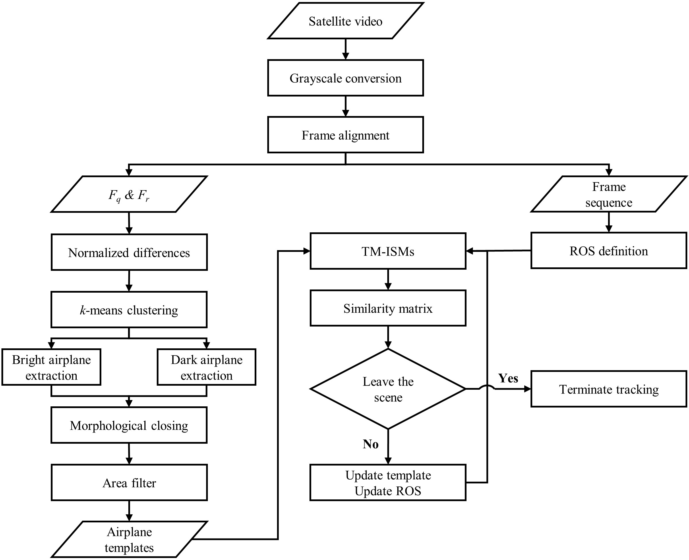
The test satellite video in this study is provided by Chang Guang Satellite Technology Co., Ltd. The original satellite video was acquired by a Jilin-1 satellite in Dubai, United Arab Emirates between 25°1′2″ N, 55°2′3″ E and 25°1′34″ N, 55°2′5″ E. The satellite video has a duration of 25 s, with a frame rate of 10 frames per second (fps) and a spatial resolution of about 1 m. The original video is cropped to cover most of the Dubai International Airport. The dimension of each cropped true-color frame is 1060 by 2750 pixels. Since our method is designed to be applicable for both true-color video (Jilin-1) and greyscale video (SkySat) data, each true-color frame of the cropped video is converted to grayscale by:

$$F=0.2989\ast F_r+0.5879\ast F_g+0.114\ast F_b$$

(1)

where F_r, F_g, and F_b represent pixel values in the red, green, and blue bands, respectively. From the second frame, all frames are geometrically aligned to the first frame to compensate for the movement of the satellite platform. This step is automatically conducted through a keypoint matching technique [30]. Specifically, SIFT keypoints extracted from two frames are matched based on the similarity of their feature vectors. Then, the coordinates of the matched keypoint pairs are used to estimate the transformation for the alignment. Figure 1 shows the first and the last (250th) frames of the aligned satellite video with all eleven moving airplanes. Airplanes 1–8, and 10 (in red rectangles) are sliding, whereas Airplanes 9 and 11 (in blue rectangles) are sliding and rotating. Airplane 5 slides for a short distance (~5 pixels) in the early 80 frames. We cannot see Airplane 10 in the last frame because it leaves the scene in the middle of the video around the 90th frame. There are three benefits of using this video to test our moving airplane detection and tracking method. First, the video contains airplanes of various sizes, from large four-engine airplanes (e.g., Airplane 1 has 60 × 80 pixels) to small two-engine airplanes (e.g., Airplane 8 has 20 × 25 pixels). Second, airplanes in this video demonstrate different motion patterns, including slide and slide with rotation. Third, this video can test the developed method with the leave-the-scene (Airplane 10) problem.

3.2. Methods

This subsection describes our method for moving airplane detection and tracking in full details. After frame alignment, normalized frame differencing labeling (NFDL) is used for moving airplane detection. The initial detection outcome is boosted by a morphological closing operation and an area filter. The templates of detected moving airplanes are input for tracking through template matching with improved similarity measures (TM-ISMs). In this process, both the template and the region of search of each airplane will be continuously updated if the airplane remains in the scene. Otherwise, the tracking will be terminated. An overview flowchart of the proposed method is shown in Figure 2. Section 3.2.1 introduces the NFDL algorithm for moving airplane detection. Section 3.2.2 presents the moving airplane tracking algorithm TM-ISMs. Section 3.2.3 analyzes the computational complexity of the TM-ISMs algorithm. Section 3.2.4 conducts an experiment to verify the rotation invariance of the improved similarity measures. Section 3.2.5 lists the metrics used to assess the performance of the developed method.

3.2.1. Moving Airplane Detection by Normalized Frame Difference Labeling

Recursive moving object detection algorithms such as ViBe [19,24] and IPGBBS [1] usually require sufficient input frames to adapt the background model before it can achieve stable detection, which is undesired for a satellite video of short duration (up to 90 s). In contrast, our NFDL algorithm adopts a non-recursive strategy for moving airplane detection that does not require background model adaption. In order to detect moving airplanes in frame F_q (the query frame), another frame F_r (the reference frame) is selected from the video to be compared with F_q. Their normalized difference image, denoted by Δ_norm, is calculated as:

$${\mathsf{\Delta }}_{norm}=\frac{\mathsf{\Delta }-\mathit{min}\left(\mathsf{\Delta }\right)}{\mathit{max}\left(\mathsf{\Delta }\right)-\mathit{min}\left(\mathsf{\Delta }\right)}\times 255$$

(2)

$$\mathsf{\Delta }=F_q-F_r$$

(3)

where Δ is the arithmetic difference array and the numerator in Equation (2) means each element in Δ is subtracted from the minimum value in Δ.

The potential range of Δ is [−255,255], and it is rescaled to Δ_norm with the range of [0,255] by Equation (2) so that negative differences, positive differences, and small differences (either positive or negative) are transformed to small positive values, large positive values, and medium positive values, respectively (Figure 3a,b). Then, the k-means clustering technique [31] is employed to group pixels of Δ_norm into three clusters. Based on their value ranges, these three clusters are further labeled with 1 (large positive values), −1 (small positive values), and 0 (medium positive values). An example of normalized difference image labeling is shown in Figure 3c, where green, red, and black pixels represent labels 1, −1, and 0, respectively. Theoretically, these different labels are caused by different combinations of pixel values in F_q and F_r (

Table 1. Possible combinations causing different pixel labels.

	1			0			−1
Fq	BRT	BRT	BCK	BRT	DRK	BCK	DRK	DRK	BCK
Fr	BCK	DRK	DRK	BRT	DRK	BCK	BRT	BCK	BRT

BRT: bright; BCK: background; DRK: dark.

). For example, the normalized difference between a bright pixel (BRT) and a dark pixel (DRK) is a large positive value and thus labeled as 1. The normalized difference between a dark pixel and a background pixel (BCK) is a small positive value and thus labeled as −1. Moreover, pixels labeled with 0 may represent either bright or dark pixels, but the small differences indicate that they are part of stationary objects. Therefore, only pixels labeled as 1 or −1 may compose moving airplanes.

To identify bright moving airplanes, we first extract pixels labeled with 1 to form a binary image I₁. Connected component labeling is then utilized to group spatially connected pixels in I₁ into different objects [32]. From the first column of Table 1, we can see that some objects in I₁ represent bright moving airplanes, whereas the others represent the background. Compared with the background, the boundary pixels of a bright airplane should have larger values than surrounding pixels; otherwise, the airplane cannot be observed. This criterion can be used to screen the objects in I₁. Specifically, for an object A in I₁, its boundary pixels, denoted by set B(A), is obtained by:

$$\begin{gathered} B\left(A\right)=A-\left(A\ominus B\right) \\ \mathit{with}A\ominus B=\left\{z|{\left(B\right)}_z\subseteq A\right\} \end{gathered}$$

(4)

where z is a pixel in A, B is a structuring element of 3 × 3 pixels, and operator – means set differencing. For the pixel z(x,y) in the set B(A), its second-order derivative in F_q, denoted by ${\nabla }^{2}f\left(x,y\right)$, takes the form:

$${\nabla }^{2}f\left(x,y\right)=f\left(x+1,y\right)+f\left(x-1,y\right)+f\left(x,y+1\right)+f\left(x,y-1\right)-4f\left(x,y\right)$$

(5)

Since a bright airplane exhibits much larger pixel values than its surrounding pixels, ${\nabla }^{2}f\left(x,y\right)$ should be negative when the pixel z(x,y) resides on the boundary. If pixels in B(A) all have negative second derivates, object A should have overall brighter boundaries than its surrounding pixels, and it is thus determined to be a bright moving airplane. Otherwise, object A is determined to be the background. In practice, instead of using the pixel-wise operation illustrated by Equation (5), we conduct a much faster operation to obtain the second-order derivatives of F_q in one calculation through the convolution with the Laplacian kernel. Let the first matrix in Figure 4 represents a subset of F_q, in which object A (inside the black polygon) has bright boundary pixels (red numbers). By convolving this matrix with a Laplacian kernel of 3 × 3, these boundary pixels will have negative values as output. Due to incomplete detection and the mixed-pixel problem, it may not be possible that all the pixels of B(A) represent the real boundary. A solution to this problem is to verify if the majority of B(A) are boundary pixels. We choose to use the 75th percentile of B(A) as an indicator of a bright moving airplane. If this number is negative, object A is determined as a bright moving airplane; otherwise, it is determined as the background.

The preceding procedure can similarly apply to the extraction of dark moving airplanes. First, pixels labeled with −1 are extracted to form a binary image I₋₁. Second, for each object in I₋₁, the second-order derivative of its boundary pixels are collected. If the 25th percentile of these second-order derivatives is positive, the object is determined as a dark moving airplane. Otherwise, the object is determined as the background. Subsequently, all moving airplanes are obtained by taking the union of bright moving airplanes and dark moving airplanes.

In order to obtain a satisfactory detection, the time interval between F_q and F_r plays an important role. The acceptable minimum time interval should meet the following criterion: during this interval, a moving airplane should be able to travel a distance longer than its length. Otherwise, the airplane may be partially detected or contains holes or gaps due to the foreground aperture problem [1,18]. Ideally, the time interval for detecting an airplane should be determined according to the average speed of the airplane, i.e., the slower the airplane is moving, the larger the time interval is required. However, such prior knowledge is not available, and the speeds of airplanes can vary in an extremely wide range. With a short test video of only 250 frames, the longest time interval is chosen in our algorithm. Specifically, Frame 250 (the last frame) is chosen as the reference frame F_r when detecting moving airplanes in Frames 1–125, whereas Frame 1 (the first frame) is chosen as the reference frame when detecting moving airplanes in Frames 126–250.

To further deal with the foreground aperture problem, a morphological closing operation is used to fill possible holes and gaps. Additionally, undesired small false alarms may exist with detected airplanes. These false alarms result from the radiometric variation of pixels in two differencing frames (mainly caused by the sun glint) and the imperfect geometrical registration. Therefore, the detection outcomes are further screened by an area filter with a threshold, which is set to be smaller than an airplane while larger than any false alarm. A detected object with an area smaller than the threshold will not be considered as a moving airplane and thus be excluded from the future tracking process.

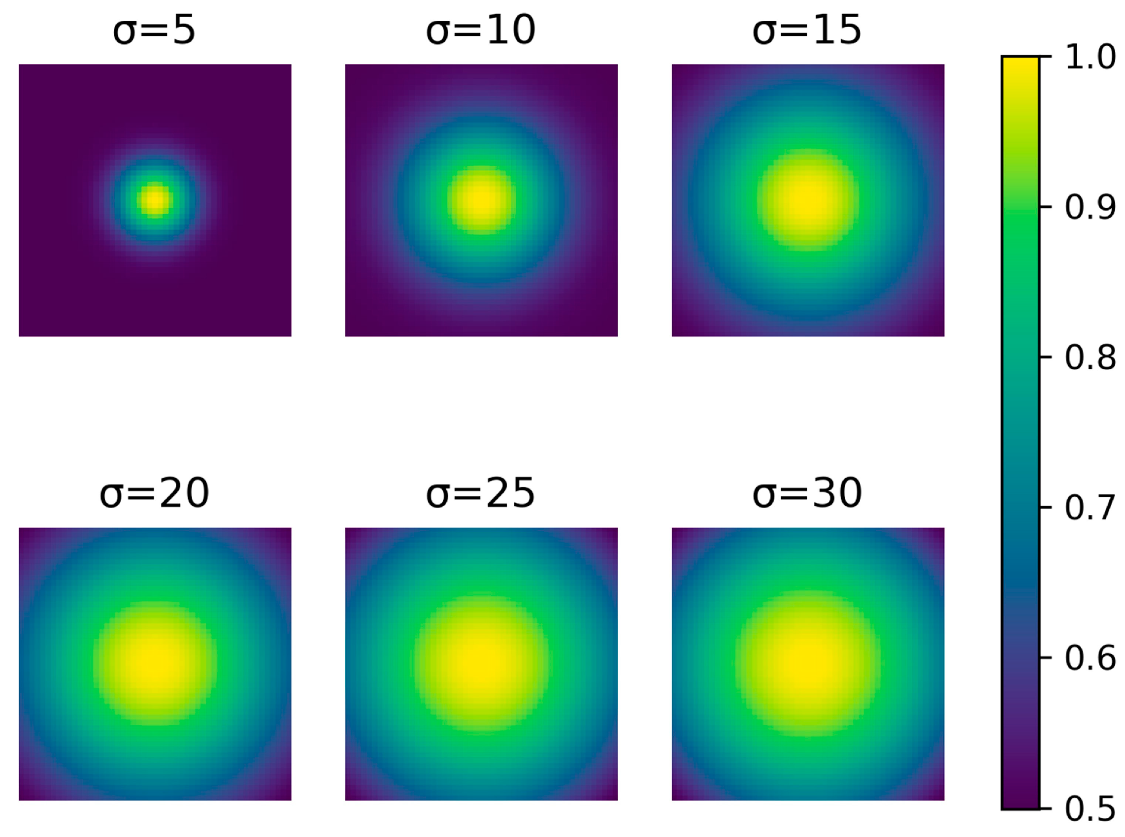
3.2.2. Moving Airplane Tracking by Template Matching

In this study, the template matching (TM) technique is adopted to track moving airplanes. Specifically, the cropped image of each detected moving airplane is referred to as a template and compared with subsets of each input video frame to find the new location of the airplane, which maximizes the similarity with the template. For each moving airplane, its template extent is initially defined based on the bounding box extracted by NFDL and frequently updated by tracking the airplanes in the frame sequence. Since the geographic coverage of a satellite video frame can be extremely large, it would be computationally costly to locate a template over an entire frame. It is necessary to define a region of search (ROS) in an input frame for each template. For an airplane in frame F_t, the upper left and lower right coordinates of its region of search, ROS_t, is represented as

$$RO{S}_t=\left(UL-\epsilon -L_t,LR+\epsilon -L_t\right)$$

(6)

where UL and LR represent the upper left and lower right coordinates of the template, respectively, ε controls the size of ROS_t, and L_t is the translation estimated by the previous tracking of the airplane. The template is moved pixel by pixel in ROS_t to calculate the similarity with each overlapped subset [33,34]. Traditional similarity measures (TSMs) have been used for TM [35,36,37], such as normalized cross-correlation (NCC), zero-mean normalized cross-correlation (ZNCC), and normalized squared difference (NSD). Collectively, they are referred to as TM-TSMs. When an airplane in ROS_t has a different orientation to the same airplane in the template, the tracking may easily fail due to the low rotation invariance of these TSMs [38,39]. To address this, we improve their rotation invariance based on the following observation. Given some degree of rotation of an object, pixels closer to the rotation center will move less from their original positions, whereas pixels farther away from the rotation center will move more. Therefore, to enhance the rotation invariance, during the computation of similarity, the pixels closer to the rotation center should be given higher weights, whereas pixels farther away from the rotation center should be given lower weights. This is achieved by introducing a Gaussian weighting plane in the similarity calculation, wherein the center of the Gaussian weighting plane has the highest weight because it corresponds to the rotation center, which remains constant in the rotation, and the weights for other pixels are inversely related to their distance from the rotation center. The Gaussian weighting plane G of a template is defined as:

$$\begin{gathered} G={\left[g\left(u,v\right)\right]}_{m\times n} \\ withg\left(u,v\right)=A·exp(\frac{-{\left|d\right|}^2}{2{\sigma }^2}) \end{gathered}$$

(7)

where (m, n) is template size, A the amplitude, and d the Euclidean distance from pixel (u, v) to the center of the template. Figure 5 illustrates Gaussian weighting planes with different standard deviation σ (from 5 to 30 with an increasing step of 5) and a constant amplitude of 1. With a smaller σ, higher weights are more concentrated toward the center of the Gaussian weighting plane. In contrast, with a larger σ, higher weights are spread out across the Gaussian weighting plane. Intuitively, the standard deviation σ should be estimated according to the degree of rotation. For an object with a large rotation angle, since the relative movement of the pixels farther from the rotation center is larger, only pixels very close to the center should be given higher weights, so a smaller σ should be chosen. In contrast, for a slightly rotated object, the relative movement of the pixels farther from the rotation center is comparatively less, and thus those pixels should also be given higher weights, so a larger σ should be chosen.

Subsequently, the developed Gaussian weighted normalized cross-correlation (GWNCC) between a template Z and a subset S, is calculated as:

$${\gamma }_{GWNCC}=\frac{{\sum }_{x,y}{Z}_G\left(x,y\right)S_G\left(x,y\right)}{\sqrt{{\sum }_{x,y}{Z}_G{}^2\left(x,y\right)\ast {\sum }_{x,y}{S}_G{}^2\left(x,y\right)}}$$

(8)

where Z_G and S_G are Gaussian weighted Z and S, respectively. Since GWNCC is a variation of NCC, it is also within the range of [0, 1] with 1 indicating Z and S are identical. Similarly, the Gaussian weighted zero-normalized cross-correlation (GWZNCC) is developed to improve the rotation invariance of ZNCC. Since the ZNCC has a range of [−1, 1], the GWZNCC is rescaled to the range [0, 1] by:

$${\gamma }_{GWZNCC}=max(0,\frac{{\sum }_{x,y}\left[Z_G\left(x,y\right)-\overline{T_G}\right]\left[Z_G\left(x,y\right)-\overline{S_G}\right]}{\sqrt{{\sum }_{x,y}{\left[Z_G\left(x,y\right)-\overline{Z_G}\right]}^2{\sum }_{x,y}{\left[S_G\left(x,y\right)-\overline{S_G}\right]}^2}})$$

(9)

where $\overline{Z_G}$ and $\overline{S_G}$ are the mean values of Z_G and S_G, respectively, and the max function converts negative values to 0. Additionally, the developed Gaussian weighted normalized squared difference (GWNSD) can also be defined by:

$${\gamma }_{GWNSD}=1-\frac{{\sum }_{x,y}{\left(Z_G\left(x,y\right)-S_G\left(x,y\right)\right)}^2}{\sqrt{{\sum }_{x,y}{Z}_G{}^2\left(x,y\right)\ast {\sum }_{x,y}{S}_G{}^2\left(x,y\right)}}$$

(10)

where ${\gamma }_{GWNSD}$ is within the range of [0, 1] with 1 indicating Z and S are identical. By using one of the improved similarity measures, all subsets in ROS_t are compared with Z to form a similarity matrix $\mathit{S}\mathit{I}{\mathit{M}}_t={\left[\gamma \right]}_{\left(m^{\prime }-m+1\right)\times \left(n^{\prime }-n+1\right)}$, where (m′,n′) represents the size of ROS_t. In SIM_t, the location of highest similarity, p_t, is found by:

$$p_t=\underset{i,j}{\mathit{max}}\mathit{S}\mathit{I}{\mathit{M}}_t\left(i,j\right)$$

(11)

When an airplane is leaving the scene or occluded by another object, the similarity at p_t drops dramatically. This situation can be monitored by applying a predetermined threshold λ to the calculated similarity. Specifically, p_t is determined as the new location of the moving airplane if the similarity at p_t is larger than λ; otherwise, the tracking for this airplane is terminated. In practice, the value of λ should be carefully selected. If λ is too small, the tracking may not be terminated when the airplane leaves the scene. If λ is too large, other types of movements such as slide and rotation can be mistakenly treated as leave-the-scene.

3.2.3. Computational Complexity Analysis

Collectively, we name GWNCC, GWZNCC, and GWNSD as improved similarity measures (ISMs). The computation of TM-ISMs mainly composes of Gaussian weighting plane definition and similarity calculation. For an airplane template of size (m,n), the Gaussian weighting plane is calculated after moving airplane detection with the complexity of $𝒪$(mn), which poses very little impact on the overall computational cost. With an airplane template of size (m,n), the complexity to find the best match in a ROS of size (m′,n′) is $𝒪$((m′ − m + 1)(n′ − n + 1)). Since the ISMs are improved based on TSMs, they demonstrate the same level of complexity as their counterparts.

3.2.4. Rotation Invariance Assessment

Collectively, we name GWNCC, GWZNCC, and GWNSD as improved similarity measures (ISMs). Compared with TSMs, ISMs are expected to exhibit better rotation invariance. To verify this, an experiment is conducted with three airplanes of different sizes (labeled with 1, 4, and 8 in Figure 1). Subsets of the airplanes are cropped from a video frame. Each subset is artificially rotated from −40° to 40°, with an increasing step of 10° (Figure 6). We then calculate the similarity between each subset and its rotated version by separately using TSMs and ISMs. Meanwhile, the value of σ is set from 1 to 20, with an increasing step of 2 for optimization. The results will be discussed in detail in the next section.

3.2.5. Accuracy Assessment Metrics

The result of moving airplane detection is assessed by the standard quantitative metrics, including true positives (TP), false positives (FP), false negatives (FN), precision, recall, and F₁ score. Precision, re-call, and F₁ score are defined as:

$$precision=\frac{TP}{TP+FP}$$

(12)

$$recall=\frac{TP}{TP+FN}$$

(13)

$$F_{1}score=2\ast \frac{precision\ast recall}{precision+recall}$$

(14)

Note that if a moving airplane is split into multiple parts, only one part is treated as TP, while other parts are treated as FPs. This consideration can help us to assess the integrity of the detected airplanes.

We use the area under the curve (AUC) of the precision plot to assess the result of moving airplane tracking. The precision plot is defined as the proportion of frames where the center location errors (CLE) are under a range of thresholds. According to Wu et al. [40], CLE is defined as the Euclidean distance between the center of tracked bounding boxes and the center of ground truths. In general, when the tracked bounding boxes are closer to the ground truths (smaller model drift), smaller CLEs are obtained, leading to a larger AUC.

4. Experimental Results

The developed method is utilized to detect and track the eleven moving airplanes in the satellite video. The first subsection compares the results of NFDL with those of existing algorithms used for detecting moving objects with satellite videos. The second subsection presents the results of the rotation invariance assessment. The third subsection presents the results of moving airplane tracking by using TM-TSMs and TM-ISMs and compares the performance of TM-ISMs with six state-of-the-art algorithms designed for either ordinary video tracking or satellite video tracking.

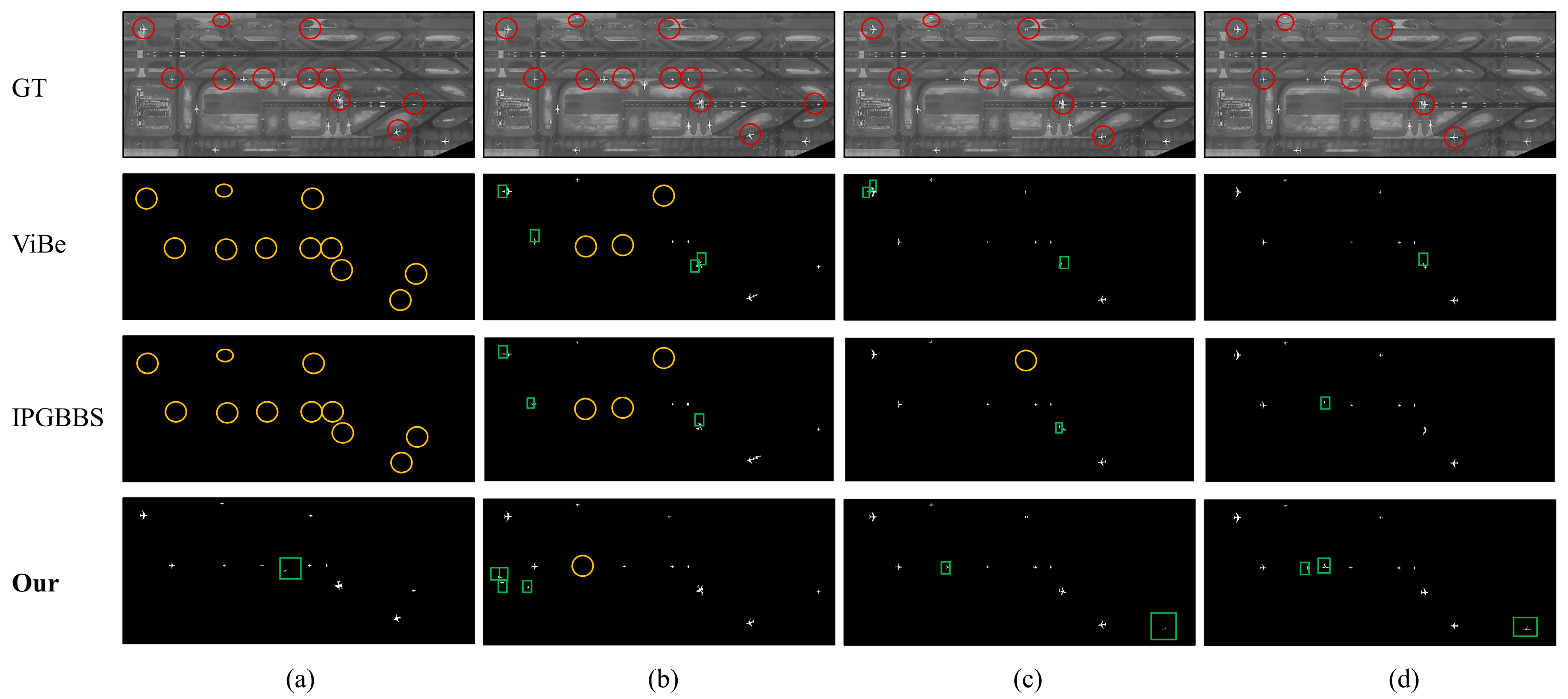
4.1. Results of Moving Airplane Detection

As discussed before, the time interval between the query frame and the reference frame is the key role for NFDL, and a large time interval can effectively address the foreground aperture problem. Therefore, for each query frame, its most distant frame is selected as the reference frame. The performance of NFDL is compared to that of both ViBe and IPGBBS. ViBe and its variants have the highest accuracy for moving car detection in satellite video data [10,23], while IPGBBS has the highest accuracy for detecting moving airplanes compared with Codebook [41], Mixture of Gaussian [42], and ViBe [19,24]. The suggested parameter values used for ViBe and IPGBBS are obtained from [1] and [3], respectively. The preliminary detection results of these three algorithms are further boosted by the morphological closing with a structuring element of 7 × 7 pixels and an area filter with a threshold of 60 pixels, which is smaller than the smallest airplane while larger than the false alarms. The boosted results of moving airplane detection in the 1st, 67th, 154th, and the 248th frames are shown in Figure 7, and corresponding quantitative evaluations are summarized in

Table 2. Quantitative evaluation results of moving airplane detection.

	Frame ID	1	67	154	248	Total	Frame ID	1	67	154	248	Average
	GT	11	11	9	9	40
ViBe	TP	0	8	9	9	26	Precision	0.77	0.67	0.75	0.90	0.76
IPGBBS		0	8	8	9	25		0.84	0.73	0.89	0.90	0.83
Our		11	10	9	9	39		0.92	0.71	0.82	0.75	0.80
ViBe	FP	0	4	3	1	8	Recall	0.91	0.73	1.00	1.00	0.65
IPGBBS		0	3	1	1	5		0.87	0.73	0.89	1.00	0.63
Our		1	4	2	3	10		1.00	0.91	1.00	1.00	0.98
ViBe	FN	11	3	0	0	14	F1 score	0.84	0.70	0.86	0.95	0.70
IPGBBS		11	3	1	0	15		0.86	0.73	0.89	0.95	0.71
Our		0	1	0	0	1		0.96	0.80	0.90	0.86	0.88

GT: ground truth.

. Since ViBe and IPGBBS cannot detect any object in the 1st frame, their demonstrated precision and recall for this frame are obtained as the averaged performance of the other three frames.

The first row of Figure 7 displays the 40 ground truths (in red circles) in four selected video frames. Both the 154th and 248th frames contain nine moving airplanes after Airplane 5 has stopped and Airplane 10 has left the study area. The second to fourth rows of Figure 7 demonstrate the detection results by using ViBe, IPGBBS, and our algorithm, while FNs (missing detection) and FPs (incorrect detection) are inside yellow circles and green rectangles, respectively. Since both ViBe and IPGBBS adopt recursive background models, they cannot detect all the airplanes in the early stage of the video (1st and 67th frames). In the 154th frame, ViBe detects all moving airplanes with 3 FPs, while IPGBBS detects eight of the nine airplanes with 1 FP. Since ViBe produces more FPs than IPGBBS over the four selected frames, it possesses lower average precision and F₁ score. In the 1st, 154th, and 248th frames, NFDL successfully detects all the moving airplanes. Compared with both ViBe and IPGBBS, NFDL has the highest values of recall for all four frames. Overall, NFDL yields the most accurate detection result with the highest recall of 0.98 and the highest F₁ score of 0.88.

The detected extent of an airplane is directly utilized for defining its template and thus greatly affects the subsequent tracking process. When an airplane is only partially detected, its defined template may not contain the whole airplane. Figure 8 shows the zoom-in view of all the airplanes detected by the three algorithms in the 248th frame. In terms of preserving the shapes of airplanes, ViBe has the poorest performance, whereas the NFDL algorithm demonstrates the best performance. Therefore, NFDL is expected to deliver the best templates for tracking.

4.2. Rotation Invariance Assessment

In Section 3.2.4, three airplanes of different sizes (small, medium, and big) are selected from the test video to calculate the similarity with their rotated versions using TSMs and ISMs. The results are summarized in Figure 9, where green lines represent TSM similarities, and 3D surfaces represent ISM similarities. In each subfigure, the highest similarity is observed when the rotation degree is 0, which is because an airplane is compared with itself. With an increased rotation angle, the similarities of all measures decrease, especially for ZNCC (second row of Figure 9). With the same rotation angle and an appropriately small value of σ, all 3D surfaces are higher than the corresponding green lines, indicating ISMs possess better rotation invariance than TSMs. For all ISMs, their resultant similarities decrease with the increase of σ. When σ is unduly large, the similarities of GWZNCC and GWNSD drop dramatically and could be even lower than their counterparts. With increased σ, the similarities of GWNCC decrease with a lower rate than that of both GWZNCC and GWNSD, which means that GWNCC has the best performance for maintaining high rotation invariance. Additionally, there is no clear pattern between airplane size and the calculated similarities. GWNCC and GWNSD have the best performance with the small airplane and the worst performance with the medium airplane, whereas GWZNCC has the best and worst performance with the big airplane and the small airplane, respectively. Overall, high rotation invariance is observed when σ is in the proper range of [3,7] for all airplanes. Within this range, all the ISMs maintain very high similarities (higher than 0.85) even with a large rotation angle of 40°, demonstrating notably better rotation invariance than their counterparts.

4.3. Results of Moving Airplane Tracking

From the detection result in the first frame (the fourth row of Figure 7a), templates of the eleven moving airplanes are extracted (after omitting the only FP in the green rectangle). We first compare the tracking results by using TM-TSMs and TM-ISMs. The take-off or landing speed of an airplane is lower than 300 km/h, and the longest distance an airplane travels between two consecutive frames (0.1 s) cannot be longer than 8.3 m. For this reason, the value of ε is set at 10 pixels (about 10 m) to make sure it is larger than the longest inter-frame travel distance. The value of ε, which controls the size of ROS, is set to 20 pixels to compensate for the varying speeds of airplanes. Based on Figure 9, the Gaussian weighting planes are created with a standard deviation (σ) of 5. With this standard deviation, all the ISMs maintain similarities higher than 0.85. Therefore, the threshold λ for TM-ISMs is set to 0.8, which is slightly lower than 0.85 to accommodate mixed pixel and lossy compression problems. Figure 10 shows the tracking results in the last frame when Airplane 10 has left the scene. The green bounding boxes represent ground truths from the first frame of the video. The magenta bounding boxes show the tracking results using TM-TSMs, and the red bounding boxes demonstrate the tracking results using TM-ISMs. For Airplanes 1–9 and 11, we calculate the total CLEs between ground truths and tracked bounding boxes over all frames, and the resultant AUCs are summarized in

Table 3. Quantitative evaluations of the tracking results by using TM and P-SIFT KM algorithms.

Algorithm	TM-TSMs			TM-ISMs
Similarity measure	NCC	ZNCC	NSD	GWNCC	GWZNCC	GWNSD
AUC	0.672	0.684	0.708	0.921	0.921	0.912

.

Based on TM-TSMs, only Airplanes 2–4 are successfully tracked with small model drift, whereas the tracking for other airplanes results in large model drift. Due to the low rotation invariance of TSMs, model drift is aggravated by the rotation. Consequently, the largest model drift is observed from the tracking of Airplanes 9 and 11, which are sliding and rotating. As a result, all TM-TSMs produce small AUCs. In contrast, TM-ISMs successfully track all the eleven airplanes with small model drift. For TM-GWNSD, the model drift for Airplane 9 is a few pixels larger than that of TM-GWNCC and TM-GWZNCC. This is indicated in Figure 9c, where GWNSD demonstrates slightly lower rotation invariance than GWNCC and GWZNCC for the big airplane. Overall, all TM-ISMs produce larger AUCs than their counterparts, and both TM-GWNCC and TM-GWZNCC exhibit the largest AUCs of 0.921. Additionally, there are no tracked bounding boxes for Airplane 10 with TM-ISMs because the tracking process is terminated as soon as the airplane leaves the scene. Therefore, TM-ISMs have successfully solved the leave-the-scene problem.

Table 4. Quantitative evaluations of different tracking algorithms.

Algorithm	Leave-the-Scene	AUC	FPS	RT
KCF [26]	√	0.950	53.60	51.10
P-SIFT KM [1]	×	0.895	216.12	12.67
MOSSE [29]	unknown	0.466	93.48	29.30
TLD [28]	unknown	0.289	2.63	1041.44
MIL [27]	×	0.913	7.99	342.80
Meanshift [25]	×	0.831	31.23	87.70
TM-GWNSD	√	0.912	448.28	6.11
TM-GWZNCC	√	0.921	392.41	6.98
TM-GWNCC	√	0.921	470.62	5.82

RT: runtime in seconds.

summarizes the AUCs of TM-ISMs and state-of-the-art algorithms, including kernelized correlation filter (KCF) [26], P-SIFT keypoint matching (P-SIFT KM) [1], minimum output sum of squared error (MOSSE) [29], tracking-learning-detection (TLD) [28], multiple instance learning (MIL) [27],and Meanshift [25]. The fourth column of Table 4 gives the average tracking speed represented by the average number of frames per second (FPS) for each airplane, and the last column gives the total run time for tracking all the eleven airplanes in the test video. In our experiment, both MOSSE and TLD lost Airplane 10 before it leaves the study area. Therefore, their capability to handle the leave-the-scene problem is unknown. Table 4 shows that TLD possesses the lowest AUC of 0.289. P-SIFT KM, MIL, and Meanshift fail to terminate the tracking after Airplane 10 leaves. Both TM-NCC and TM-ZNCC achieve a very high AUC of 0.921, comparable to that of KCF. More importantly, all TM-ISMs demonstrate the fastest tracking speed among all algorithms, especially TM-GWNCC, which is approximately nine times faster than KCF.

The trajectories of moving airplanes are depicted based on the tracking results with TM-GWNCC (Figure 11). Each trajectory is derived by sequentially connecting the airplane’s tracked locations in all frames. These trajectories agree well with the visual observation of the test video. Specifically, the trajectories of Airplanes 1–8 and 10 demonstrate only slide with no evident rotation, whereas the trajectories of Airplanes 9 and 11 show both slide and rotation.

5. Discussion

In moving airplane detection, normalized frame differences are grouped into three clusters. After comparing the performance of existing clustering algorithms, k-means was chosen for two reasons. First, k-means can run very fast over a large video frame (especially compared with DBSCAN [43]), preferable for real-time detection. Second, the number of clusters is preset with k-means rather than automatically estimated as in many other algorithms. Similar to some of the other algorithms, k-means may fail to provide reasonable clustering when pixel labels are extremely unbalanced. Although k-means always delivers the desired result in our test video, NFDL would benefit from a more effective clustering algorithm to deal with the imbalanced data problem.

For traditional remote sensing studies, the data processing speed may not be a major concern because data is often processed after being transmitted back to a ground station. In satellite videography, many tracking tasks can be time-sensitive, and thus real-time processing is desirable. The high efficiency of our method shows great potential for real-time monitoring if deployed onboard video satellites. In this case, a ground station can choose to directly receive the real-time locations of moving objects instead of large-volume video data if so desired.

For a spaceborne platform, the quality of its remote sensing data can be impacted by inclement weather, which will inevitably limit the performance of the proposed method. In cases of heavy cloud and dust, the contrast of the delivered satellite video may be degraded, and NFDL may miss the small airplanes because they can be easily melted into the background. With the ongoing resolution improvement of satellite videography and the increased satellite video data availability, our moving airplane detection and tracking method can further take advantage of these developments to deliver better performance. Our tracking algorithm is tested in only one satellite video in this study. With the increased revisit capability of satellite videography, how to identify and track the same airplane in a sequence of videos remains an interesting research question.

6. Conclusions

Satellite videography, as an emerging technology, provides a new perspective to observe the earth’s surface, which enables us to monitor moving objects from space. While attention has been given to detect and track moving cars, airplanes have not been treated in much detail. This paper describes a method to detect and track moving airplanes in a satellite video. First, we developed a Normalized Frame Difference Labeling (NFDL) algorithm for moving airplane detection. NFDL adopts a non-recursive strategy to provide stable detection throughout the whole video. Second, we used template matching to track the detected moving airplanes in the frame sequence. In this stage, the rotation invariance of TSMs was improved by introducing a Gaussian weighting plane. An experiment was conducted by applying the developed method to detect and track eleven moving airplanes in the test video. For moving airplane detection, NFDL produced the highest recall and F₁ score and also demonstrated the best capability to preserve the shapes of detected airplanes. For moving airplane tracking, all the ISMs demonstrated notably better rotation invariance than their counterparts, which contributed to more accurate tracking with better model drift suppression. With the fastest tracking speed, TM-ISMs achieved tracking accuracy better than or comparable to state-of-the-art algorithms.

References

1. Shi, F.; Qiu, F.; Li, X.; Tang, Y.; Zhong, R.; Yang, C. A Method for Detecting and Tracking Moving Airplanes from a Satellite Video. Remote Sens. 2020, 12, 2390. [Google Scholar] [CrossRef]
2. Shao, J.; Du, B.; Wu, C.; Zhang, L. Tracking Objects from Satellite Videos: A Velocity Feature Based Correlation Filter. IEEE Trans. Geosci. Remote Sens. 2019, 57, 7860–7871. [Google Scholar] [CrossRef]
3. Yang, T.; Wang, X.; Yao, B.; Li, J.; Zhang, Y.; He, Z.; Duan, W. Small moving vehicle detection in a satellite video of an urban area. Sensors 2016, 16, 1528. [Google Scholar] [CrossRef] [PubMed] [Green Version]
4. Kopsiaftis, G.; Karantzalos, K. Vehicle detection and traffic density monitoring from very high resolution satellite video data. In Proceedings of the IEEE International Geoscience and Remote Sensing Symposium (IGARSS), Milan, Italy, 26–31 July 2015; pp. 1881–1884. [Google Scholar]
5. Guo, Y.; Yang, D.; Chen, Z. Object Tracking on Satellite Videos: A Correlation Filter-Based Tracking Method with Trajectory Correction by Kalman Filter. IEEE J. Sel. Top. Appl. Earth Obs. Remote Sens. 2019, 12, 3538–3551. [Google Scholar] [CrossRef]
6. Du, B.; Cai, S.; Wu, C.; Zhang, L.; Dacheng, T. Object Tracking in Satellite Videos Based on a Multi-Frame Optical Flow Tracker. IEEE J. Sel. Top. Appl. Earth Obs. Remote Sens. 2019, 12, 3043–3055. [Google Scholar] [CrossRef] [Green Version]
7. Ahmadi, S.A.; Ghorbanian, A.; Mohammadzadeh, A. Moving vehicle detection, tracking and traffic parameter estimation from a satellite video: A perspective on a smarter city. Int. J. Remote Sens. 2019, 40, 8379–8394. [Google Scholar] [CrossRef]
8. Shao, J.; Du, B.; Wu, C.; Zhang, L. Can We Track Targets From Space? A Hybrid Kernel Correlation Filter Tracker for Satellite Video. IEEE Trans. Geosci. Remote Sens. 2019, 57, 8719–8731. [Google Scholar] [CrossRef]
9. Du, B.; Sun, Y.; Cai, S.; Wu, C.; Du, Q. Object Tracking in Satellite Videos by Fusing the Kernel Correlation Filter and the Three-Frame-Difference Algorithm. IEEE Geosci. Remote Sens. Lett. 2018, 15, 168–172. [Google Scholar] [CrossRef]
10. Zhang, J.; Jia, X.; Hu, J. Motion Flow Clustering for Moving Vehicle Detection from Satellite High Definition Video. In Proceedings of the 2017 International Conference on Digital Image Computing: Techniques and Applications (DICTA), Sydney, Australia, 29 November–1 December 2017; pp. 1–7. [Google Scholar]
11. Mou, L.; Zhu, X.; Vakalopoulou, M.; Karantzalos, K.; Paragios, N.; Le Saux, B.; Moser, G.; Tuia, D. Multitemporal Very High Resolution from Space: Outcome of the 2016 IEEE GRSS Data Fusion Contest. IEEE J. Sel. Top. Appl. Earth Obs. Remote Sens. 2017, 10, 3435–3447. [Google Scholar] [CrossRef] [Green Version]
12. Ahmadi, S.A.; Mohammadzadeh, A. A simple method for detecting and tracking vehicles and vessels from high resolution spaceborne videos. In Proceedings of the Joint Urban Remote Sensing Event (JURSE), Dubai, UAE, 6–8 March 2017; pp. 1–4. [Google Scholar] [CrossRef]
13. D’Angelo, P.; Kuschk, G.; Reinartz, P. Evaluation of skybox video and still image products. Int. Arch. Photogramm. Remote Sens. Spat. Inf. Sci. 2014, 40, 95. [Google Scholar] [CrossRef] [Green Version]
14. Leitloff, J.; Hinz, S.; Stilla, U. Vehicle detection in very high resolution satellite images of city areas. IEEE Trans. Geosci. Remote Sens. 2010, 48, 2795–2806. [Google Scholar] [CrossRef]
15. Liu, W.; Yamazaki, F.; Vu, T.T. Automated Vehicle Extraction and Speed Determination From QuickBird Satellite Images. IEEE J. Sel. Top. Appl. Earth Obs. Remote Sens. 2011, 4, 75–82. [Google Scholar] [CrossRef]
16. Salehi, B.; Zhang, Y.; Zhong, M. Automatic moving vehicles information extraction from single-pass worldView-2 imagery. IEEE J. Sel. Top. Appl. Earth Obs. Remote Sens. 2012, 5, 135–145. [Google Scholar] [CrossRef]
17. Teutsch, M.; Kruger, W. Robust and fast detection of moving vehicles in aerial videos using sliding windows. In Proceedings of the IEEE Computer Society Conference on Computer Vision and Pattern Recognition Workshops, Boston, MA, USA, 7–12 June 2015; pp. 26–34. [Google Scholar]
18. Bouwmans, T. Traditional and recent approaches in background modeling for foreground detection: An overview. Comput. Sci. Rev. 2014, 11, 31–66. [Google Scholar] [CrossRef]
19. Barnich, O.; van Droogenbroeck, M. ViBe: A universal background subtraction algorithm for video sequences. IEEE Trans. Image Process. 2010, 20, 1709–1724. [Google Scholar] [CrossRef] [Green Version]
20. Hu, Z.; Yang, D.; Zhang, K.; Chen, Z. Object tracking in satellite videos based on convolutional regression network with appearance and motion features. IEEE J. Sel. Top. Appl. Earth Obs. Remote Sens. 2020, 13, 783–793. [Google Scholar] [CrossRef]
21. Piccardi, M. Background subtraction techniques: A review. In Proceedings of the IEEE International Conference on Systems, Man and Cybernetics, Hague, The Netherlands, 10–13 October 2004; Volume 4, pp. 3099–3104. [Google Scholar]
22. Elhabian, S.Y.; El-Sayed, K.M.; Ahmed, S.H. Moving object detection in spatial domain using background removal techniques-state-of-art. Recent Patents Comput. Sci. 2008, 1, 32–54. [Google Scholar] [CrossRef]
23. Cheung, S.C.S.; Kamath, C. Robust techniques for background subtraction in urban traffic video. Vis. Commun. Image Process. 2004, 5308, 881–892. [Google Scholar] [CrossRef]
24. Barnich, O.; van Droogenbroeck, M. ViBe: A powerful random technique to estimate the background in video sequences. In Proceedings of the IEEE International Conference on Acoustics, Speech and Signal Processing, Taipei, Taiwan, 19–24 April 2009; pp. 945–948. [Google Scholar]
25. Comaniciu, D.; Ramesh, V.; Peter, M. Real-time tracking of non-rigid objects using mean shift. In Proceedings of the IEEE Conference on Computer Vision and Pattern Recognition, Hilton Head Island, SC, USA, 15 June 2000; Volume 2, pp. 142–149. [Google Scholar]
26. Henriques, J.F.; Caseiro, R.; Martins, P.; Batista, J. High-speed tracking with kernelized correlation filters. IEEE Trans. Pattern Anal. Mach. Intell. 2014, 37, 583–596. [Google Scholar] [CrossRef] [Green Version]
27. Babenko, B.; Yang, M.H.; Serge, B. Visual tracking with semi-supervised online weighted multiple instance learning. In Proceedings of the IEEE Conference on computer vision and Pattern Recognition, Miami, FL, USA, 20–25 June 2009; pp. 983–990. [Google Scholar]
28. Kalal, Z.; Mikolajczyk, K.; Matas, J. Tracking-learning-detection. IEEE Trans. Pattern Anal. Mach. Intell. 2011, 34, 1409–1422. [Google Scholar] [CrossRef] [Green Version]
29. Bolme, D.S.; Beveridge, J.R.; Draper, B.A.; Lui, Y.M. Visual object tracking using adaptive correlation filters. In Proceedings of the IEEE Computer Society Conference on Computer Vision and Pattern Recognition, San Francisco, CA, USA, 13–18 June 2010; pp. 2544–2550. [Google Scholar]
30. Ma, W.; Wen, Z.; Wu, Y.; Jiao, L.; Gong, M.; Zheng, Y.; Liu, L. Remote Sensing Image Registration with Modified SIFT and Enhanced Feature Matching. IEEE Geosci. Remote Sens. Lett. 2017, 14, 3–7. [Google Scholar] [CrossRef]
31. Jain, A.K. Data clustering: 50 years beyond K-means. Pattern Recognit. Lett. 2010, 31, 651–666. [Google Scholar] [CrossRef]
32. He, L.; Chao, Y.; Suzuki, K. A Run-based one-and-a-half-scan connected-component labeling algorithm. Int. J. Pattern Recognit. Artif. Intell. 2010, 24, 557–579. [Google Scholar] [CrossRef]
33. Liwei, W.; Yan, Z.; Jufu, F. On the Euclidean distance of images. IEEE Trans. Pattern Anal. Mach. Intell. 2005, 27, 1334–1339. [Google Scholar] [CrossRef]
34. Nakhmani, A.; Tannenbaum, A. A new distance measure based on generalized Image Normalized Cross-Correlation for robust video tracking and image recognition. Pattern Recognit. Lett. 2013, 34, 315–321. [Google Scholar] [CrossRef] [PubMed] [Green Version]
35. Mahmood, A.; Khan, S. Correlation Coefficient Based Fast Template Matching Through Partial Elimination. IEEE Trans. Image Process. 2011, 21, 2099–2108. [Google Scholar] [CrossRef]
36. Briechle, K.; Hanebeck, U.D. Template matching using fast normalized cross correlation. In Optical Pattern Recognition XII; International Society for Optics and Photonics: Bellingham, DC, USA, 2001; Volume 4387, pp. 95–102. [Google Scholar]
37. Schweitzer, H.; Bell, J.W.; Wu, F. Very fast template matching. In European Conference on Computer Vision; Springer: Berlin/Heidelberg, Germany, 2002; pp. 358–372. [Google Scholar]
38. Goshtasby, A. Template Matching in Rotated Images. IEEE Trans. Pattern Anal. Mach. Intell. 1985, 338–344. [Google Scholar] [CrossRef]
39. Tsai, D.M.; Tsai, Y.H. Rotation-invariant pattern matching with color ring-projection. Pattern Recognit. 2002, 35, 131–141. [Google Scholar] [CrossRef]
40. Wu, Y.; Lim, J.; Yang, M.H. Online object tracking: A benchmark. In Proceedings of the IEEE Computer Society Conference on Computer Vision and Pattern Recognition, Portland, OR, USA, 23–28 June 2013; pp. 2411–2418. [Google Scholar]
41. Kim, K.; Chalidabhongse, T.H.; Harwood, D.; Davis, L. Real-time foreground-background segmentation using codebook model. Real Time Imaging 2005, 11, 172–185. [Google Scholar] [CrossRef] [Green Version]
42. Stauffer, C.; Grimson, W.E.L. Adaptive background mixture models for real-time tracking. In Proceedings of the IEEE Computer Society Conference on Computer Vision and Pattern Recognition, Fort Collins, CO, USA, 23–25 June 1999; Volume 2, pp. 246–252. [Google Scholar] [CrossRef]
43. Ester, M.; Kriegel, H.P.; Sander, J.; Xu, X. A density-based algorithm for discovering clusters in large spatial databases with noise. In Proceedings of the Second International Conference on Knowledge Discovery and Data Mining (KDD-96), Portland, OR, USA, 2–4 August 1996; Volume 96, pp. 226–231. [Google Scholar]
Figure 1. The first frame (a) and the last frame (b) of the aligned satellite video. All eleven moving airplanes are labeled. Airplanes 1–8 and 10 in red rectangles are sliding, whereas Airplanes 9 and 11 in blue rectangles are sliding and rotating. Airplane 5 slides for a very short distance in the early 80 frames, and Airplane 10 leaves the scene around the 90th frame of the video.
Remotesensing 12 03589 g001
Figure 2. Flowchart of the proposed moving airplane detection and tracking method.
Remotesensing 12 03589 g002
Figure 3. Normalized difference image labeling: (a) normalized difference image between two frame subsets containing the same moving airplane; (b) frequencies of the normalized differences, (c) the k-means clustering technique groups normalized differences into three clusters labeled by 1 (green), −1 (red), and 0 (black).
Remotesensing 12 03589 g003
Figure 4. The Laplacian of an image subset containing object A. If A is a bright airplane, its boundary pixels should all have negative values of Laplacian.
Remotesensing 12 03589 g004
Figure 5. Gaussian weighting planes with σ values of 5, 10, 15, 20, 25, 30, and a constant amplitude of 1.
Remotesensing 12 03589 g005
Figure 6. Three airplanes of different sizes for rotation invariance assessment. (a) airplanes of different sizes, and (b) examples of their rotated versions.
Remotesensing 12 03589 g006
Figure 7. The moving object detection results in the 1st (a), 67th (b), 154th (c), and 248th (d) frames. Red circles, yellow circles, and green rectangles represent ground truths, FNs (missing detection), and FPs (incorrect detection), respectively.
Remotesensing 12 03589 g007
Figure 8. Zoom-in view of detected moving airplanes in the 248th frame. (a) ViBe, (b) IPGBBS, (c) Our algorithm.
Remotesensing 12 03589 g008
Figure 9. Similarities calculated by TSMs (green lines) and ISMs (3D surfaces) for the selected small airplane (a), medium airplane (b), and big airplane (c), respectively.
Remotesensing 12 03589 g009
Figure 10. Results of tracking airplanes in the last frame. Green bounding boxes represent ground truths in the first frame. Magenta and red bounding boxes demonstrate the tracking results by using traditional similarity measures and improved similarity measures, respectively.
Remotesensing 12 03589 g010
Figure 11. Trajectories of 11 moving airplanes delineated on the first frame.
Remotesensing 12 03589 g011