A Novel Electromagnetic Wave Rain Gauge and its Average Rainfall Estimation Method

Abstract

It is essential to accurately estimate rainfall to predict and prevent hydrological disasters such as floods. In this paper, an electromagnetic wave rain gauge system and a method to estimate average rainfall using the system’s multiple elevation observation data are presented. The compact electromagnetic wave rain gauge is a small-sized radar that performs very short-range observations using K-band dual-polarization technology. The method to estimate average rainfall is based on the concept of an average observation derived from multiple elevation scans with very short range and dual-polarization information. The proposed method was evaluated by comparing it with ground instruments, including a pit-gauge, tipping-bucket rain gauges, and a Parsivel disdrometer. The evaluation results demonstrated that the new methodology worked fairly well for various rainfall events.

1. Introduction

A reliable hydrological disaster forecast-warning system requires a more effective method to observe the spatial distribution of rainfall than can be achieved using conventional point-based rain gauges. Ground-based rain gauges have the advantage of providing continuous and direct measurements of rainfall. However, in areas where such gauges are absent, it is not possible to provide accurate information about the spatial distribution of rainfall [1,2,3,4]. In addition, rain gauge rainfall measurements tend to be underestimated in strong winds [5]. Weather radars have been suggested as an alternative to conventional ground-based rain gauges to estimate rainfall. They can cover a relatively large area and provide a high spatial and temporal sampling. In particular, the introduction of dual-polarization technology has facilitated rainfall estimations that are highly accurate [6,7,8,9,10,11,12]. A weather radar is the most commonly available, wide-area precipitation observation equipment, and is used to estimate rainfall intensity in conjunction with ground rain gauges. However, it is difficult to directly reflect rainfall at the ground level, as radar observations are conducted at elevations of several hundred meters to several kilometers above the ground. To address these issues, an electromagnetic wave rain gauge (EWRG) was developed. This is a new area rain gauge system that uses electromagnetic waves. To achieve the accuracy and spatial resolution of ground-level rainfall, the EWRG system operates at a low altitude, at a close range, and estimates the average rainfall with dual-polarization variables averaged over the observed area [13,14]. Note that micro-rain radar (MRR) can be another alternative for rainfall estimation using electromagnetic waves [15]. MRR is a vertical pointing FMCW system, while EWRG is a scanning dual-polarization system.

Typically, dual-polarization radar parameters, including reflectivity (Z_h), differential reflectivity (Z_dr), and the specific differential phase (K_dp)) are used either alone or in combination to estimate rainfall intensity. Representative quantitative precipitation estimation (QPE) algorithms for dual-polarization radar include those of the Joint Polarization Experiment (JPOLE) [7] and Colorado State University (CSU) [9,12]. The radar-based rainfall estimation method calculates the rainfall intensity for each gate from the radar data. The rainfall estimation method, which calculates rainfall intensity values per gate, may be suitable for radar systems with relatively long distances. However, it may not be appropriate to apply this method to area average rainfall estimation using EWRG data with very short distances (for example, 1–2 km or less). Therefore, it is necessary to develop a method that can more accurately calculate the rainfall intensity value through the concept of average rainfall in a very close-range observation area. In this study, we developed a method for estimating the average rainfall intensity using multiple elevation observation data obtained from the dual-polarization EWRG. The average rainfall intensity of the observed area can be estimated using mean values per elevation angle of reflectivity and the specific differential phase of multiple elevations. The average rainfall of the EWRG is the amount of rainfall estimated using the mean values of the radar parameters for the area, and this varies depending on the observation range. In this study, average rainfall was based on an area of 3.14 km² and an EWRG observation projected radius of 1.0 km was assumed.

The remainder of this paper is organized as follows. In Section 2, the system specifications of the developed EWRG prototype and scan strategy are briefly described. Section 3 describes the proposed method used to estimate the average rainfall. In Section 4, the proposed areal average rainfall estimation method is applied to various rainfall events. Comparisons are made with the results of conventional ground-based equipment, and the results are discussed. Section 5 presents a summary and conclusions.

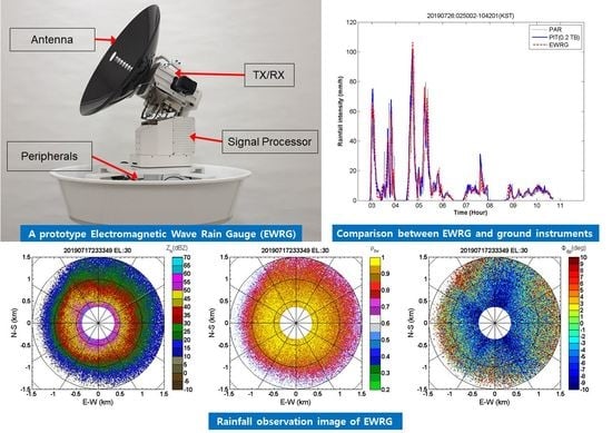
2. Description of the EWRG

2.1. EWRG Specifications

The EWRG developed in this study is an average rainfall estimation system that complements the conventional tipping bucket rain gauge. It is a compact, integrated system that combines a transmitter, receiver, and a data collection system into two assemblies (Figure 1). The system uses dual-polarization technology and operates at the K band frequency. The transmitter/receiver generates a linear frequency modulation (LFM) signal with a peak power of 4 W per channel (H/V). The parabolic dish antenna had a diameter of 50 cm and a beamwidth of 1.6°.

The system block diagram is shown in Figure 2. The intermediate frequency (IF) signals of the horizontal and vertical channels received from the transmitter/receiver of the EWRG were sampled by an analog-to-digital converter (ADC) and then converted to digital signals. They then undergo a digital down converter (DDC) and pulse compression process and are converted into I/Q data. The various observation variables are calculated from the I/Q data, and the final output is transferred to the operation control device via Ethernet. The observation variables are reflectivity (Z), radial velocity (V), spectral width (W) for each polarization, differential reflectivity (Z_dr), correlation coefficient (ρ_hv), and differential propagation phase (Φ_dp).

Table 1. Specifications of EWRG prototype.

Item	Specification
Operating frequency	24.15 GHz
Polarization	Simultaneous (H/V)
Transmit peak power	4 W/channel (H/V)
Antenna shape	Parabolic reflector (Carbon)
Antenna diameter	50 cm
Beamwidth	1.6 degree
Gain	40 dBi
Voltage standing wave ratio	<1.5:1
Driving range (deg)	0–360 (Azimuth), –2– +92 (Elevation)
Effective observation range	1.5 km
Waveform	5 MHz (LFM pulse)
Pulse width	1 μs
Pulse repetition frequency	10,000 Hz
Range resolution	7.5 m

presents the specifications of the EWRG in detail.

2.2. EWRG Scan Strategy

Given the complexity of rainfall and the vertical variability of the radar parameters, it is important to obtain low-altitude observations to reduce uncertainties in rainfall estimation [8]. However, if systems are installed close to the ground, data can be affected by topographic features, such as mountains or buildings. Generally, EWRG is installed close to the ground. Therefore, a specific scan strategy is required to minimize ground clutter effects and to enable rainfall observations to be conducted at a low altitude depending on the installation surroundings. Figure 3 shows the current scan strategy of the EWRG. Projections of each scan are shown in the XY plane. The system conducts scans at elevations of 30° (blue), 45° (red), and 60° (cyan) to estimate average rainfall. The lowest altitude, 30°, was chosen to keep the rainfall estimates consistent across multiple test sites, and 45° and 60° were chosen arbitrarily. Note that the scan strategy can be changed according to the installation location and surrounding environment.

3. EWRG Average Rainfall Estimation Method

The EWRG rainfall estimation method is based on the assumption that the spatial variability of rainfall distribution can be small at very close distances. The proposed method uses the average values of multiple elevation scan data in a very short range. At higher frequencies, such as the K band, K_dp can be an important parameter for rainfall estimation because it is not affected by propagation attenuation and the absolute calibration error of the radar system [16,17]. However, if the echo is weak, K_dp is very small and can fluctuate. In this case, Z_h can be better than K_dp. Therefore, the proposed method uses Z_h or K_dp, depending on the decision criteria described in Section 3.2.

3.1. Reflectivity Calibration

K_dp is immune to system bias, but Z_h is strongly affected by system errors. Therefore, Z_h calibration is necessary for the estimation of rainfall. In this study, we used a conventional method to monitor absolute calibration using a direct comparison of EWRG data and disdrometer measurements [18,19]. Observed Z_h values were compared with Z_h values retrieved from Parsivel data during a weak rain period (averaged observed Z_h < 35 dBZ). EWRG bias was then obtained at the best-matched bias value. Figure 4 shows an example of the comparison results of EWRG and Parsivel reflectivity after Z_h calibration. As can be seen in the figure, the EWRG Z_h peak is much smaller than Parsivel (by approximately 4–6 h) may be due to the attenuation of the radome and path. Note that the reason for selecting data during a period of weak rainfall is to minimize the impact of radome and path attenuation. The locations of Parsivel and EWRG were co-located at the Geoje field test site, and the Parsivel at the Yeoncheon site was located about 700 m away from the EWRG (see Chapter 4 for detailed layout of test sites).

3.2. EWRG Average Rainfall Estimation Procedure

The detailed process used to estimate the average rainfall is shown in Figure 5. The method consists of five main steps. (i) For inputs, Z_h and Φ_dp, as the multiple elevation scan data of the dual-polarization radar observing a very short distance, were used. The input scan observation data are observation variables obtained at elevation angles of 30°, 45°, and 60°: Z_h(30), Z_h(45), Z_h(60), Φ_dp(30), Φ_dp(45), and Φ_dp(60), respectively. (ii) Next, the mean K_dp (<K_dp>) for each elevation was retrieved from Φ_dp. The <K_dp> retrieval process is illustrated in Figure 6. Φ_dp were averaged, and then <K_dp> was calculated from a slope of averaged <Φ_dp> as $\langle K_{dp}\rangle =\frac{\mathsf{\Delta }\langle {\mathsf{\Phi }}_{dp}\left(r\right)\rangle }{2·\mathsf{\Delta }\mathrm{r}}$. (iii) Mean Z_h (<Z_h>) for each elevation was obtained using Z_h scan data; (iv) the multiple elevation means of Z_h and K_dp (μ(Z_h) and μ(K_dp)) were calculated using <Z_h> and <K_dp> for each elevation; (v) finally, according to conditions, the average rainfall intensity was estimated. In this study, μ(Z_h) of 35 dBZ and μ(K_dp) of 0.2°/km were used as threshold values. Note that in this study, attenuation correction was not applied for Z_h.

The rainfall estimation equations using reflectivity and specific differential phase are as follows:

$$\mathrm{R}\left(\mathsf{\mu }\left({\mathrm{Z}}_{\mathrm{h}}\right)\right)=\mathrm{a}{\left(\mathsf{\mu }\left({\mathrm{Z}}_{\mathrm{h}}\right)\right)}^{\mathrm{b}}$$

(1)

$$\mathrm{R}\left(\mathsf{\mu }\left({\mathrm{K}}_{\mathrm{dp}}\right)\right)=\mathrm{c}\left(\mathsf{\mu }\left({\mathrm{K}}_{\mathrm{dp}}\right)\right)$$

(2)

where Z_h (mm⁶ m⁻³) is the reflectivity factor at horizontal polarization. Parameters a, b, and c were obtained by scattering simulation using the shape model proposed by Bringi et al. [20], which is a combination of the Andsager et al. [21] and the Beard and Chuang [22] model at a temperature of 15 °C. The scatter plots of Z_h versus rainfall and K_dp versus rainfall for different elevations are shown in Figure 7. From the figures, it can be seen that Z_h does not change significantly with elevation at which K_dp varies significantly. In this study, a = 0.001, b = 0.78, and c = 21.4 were used for a frequency of 24 GHz and at an observation elevation of 45°. By assuming symmetry of scan elevations, parameters of only middle elevation are used. Note that if the scan strategy is changed, especially parameter c, must be adjusted.

4. Evaluation of EWRG Average Rainfall Estimation and Discussion

To test the EWRG, field tests for several rainfall events were conducted at multiple locations. In this paper, two main rainfall events (occurring on 17–20 July 2019 at Geoje, and on 26 July 2019 at Yeoncheon) were analyzed. A variety of ground instruments (conventional tipping bucket rain gauges, Parsivel disdrometers, and a pit-gauge) were used to evaluate the average rainfall estimation. A well-known problem associated with Parsivel is the underestimation of rainfall, especially during heavy rains. For this reason, Parsivel rainfall data were used only for qualitative evaluation in this study. Figure 8 shows the locations of the two main sites. The Geoje test site (approximately 30 m above sea level) is surrounded by the sea to the south and mountains to the north, and the Yeoncheon site (about 77 m above sea level) is located in a valley.

4.1. EWRG Field Test (Geoje)

Due to the influence of Typhoon Danas, heavy rain occurred in the southern part of the Korean Peninsula, from 17 to 20 July 2019. To evaluate the estimation of EWRG average rainfall, two tipping bucket rain gauges and one Parsivel disdrometer were installed near the EWRG. The layout of the EWRG test site is shown in Figure 9.

An example of the EWRG data obtained at 23:33:49 on 17 July 2019, is depicted in Figure 10 (where reflectivity, the correlation coefficient, and the differential phase shift are represented from left to right). The significant reduction of Z_h and ρ_hv presented in the figure with the height-range is due to heavy rain attenuation.

For a detailed analysis of the rainfall event that occurred on 17–20 July 2019, the event was further classified into three separate events, according to the time of occurrence. The first was a very heavy rainfall event that occurred from 22:05 LST on 17 July 2019, to 07:29 LST on 18 July. The second event occurred from 01:44 to 13:00 on 19 July 2019, and the third occurred from 23:10 on 2019/07/19 to 06:10 on 2019/07/20. Figure 11 shows the results of a comparative analysis of the first event. The instantaneous average rainfall intensity (mm/h) estimated by EWRG and rainfall from the rain gauge are shown in Figure 11a, and Figure 11b shows a comparison of cumulative rainfall (mm). The comparative analysis of events 2 and 3 are shown in Figure 12 and Figure 13, respectively. Figure 12a and Figure 13a show the instantaneous average rainfall intensity (mm/h) estimated by the EWRG and rain gauge, and Figure 12b and Figure 13b show a comparison of cumulative rainfall (mm). It is of note here that the EWRG rainfall is the areal-averaged rainfall, whereas that of the rain gauges is point rainfall. Figure 11 and Figure 12 show that there is little difference between EWRG-derived rainfall and rain gauge rainfall. However, for the event occurring on 20 July (Figure 13), there is an error of about 20% between EWRG and rain gauge rainfalls. These errors are considered to be due to the systemic limitation of EWRG and the spatiotemporal variability of rainfall. This system limitation is caused by the high-minimum detectable signal (MDS) due to the low transmit power and errors in the reflectivity calibration. During heavy rain, K_dp is not significantly affected by these factors, but during weak rainfall, Z_h can be greatly affected. For these reasons, the current EWRG prototype tends to underestimate weak rainfall.

4.2. EWRG Field Test (Yeoncheon)

To evaluate the EWRG’s performance, a testbed was established at the Yeoncheon SOC Demonstration Research Center of the Korea Institute of Civil Engineering and Building Technology. In addition to using a typical tipping bucket rain gauge and Parsivel disdrometer, a pit-gauge was installed to obtain more accurate ground rainfall observations at the site. The layout of the comparison testbed (complex pit-gauge and EWRG) established in the Yeoncheon SOC Demonstration Research Center is depicted in Figure 14.

On 26 July 2019, heavy rain (event 4), caused by a strong seasonal rain front, hit the central and northern parts of the Korean Peninsula, causing a downpour exceeding 100 mm/h. EWRG observation images taken at 07:08 on 26 July 2019, are shown in Figure 15 (from left to right: reflectivity, correlation coefficient, and differential phase shift). Figure 16a shows the instantaneous average rainfall intensity (mm/h) estimated by the EWRG and the rainfall intensity obtained by the ground instruments, and Figure 16b compares the cumulative rainfall (mm). In this figure, a comparison of the results of the pit-gauge (installed approximately 600 m from EWRG) and the EWRG show that, for this event, the average rainfall estimates of the EWRG were almost identical to the rainfall measured at the pit-gauge. However, as with the Geoje event, the observation results for this event demonstrated that the rainfall intensity estimation of the Parsivel disdrometer tends to be slightly underestimated.

4.3. Comprehensive Analysis

We conducted a comparative analysis between the EWRG average rainfall estimates and the data obtained from several ground instruments. Both rainfall events analyzed in this study were heavy, with instantaneous rainfall intensities of 30–100 mm/h, which are suitable for analyzing the performance of the EWRG and for determining whether it could be used to assist in the prevention of hydrological disasters. The errors between the total cumulative average rainfalls obtained by the EWRG and the ground rain gauge are summarized in

Table 2. Error comparison of total cumulative rainfall between the EWRG and ground-based equipment (Pit-Gauge, Tipping gauge).

Event	Pit-Gauge (mm)	Tipping Gauge (0.2) (mm)	EWRG (mm)	Error (%)
1	-	48.9	44.2	–9.6
2	-	51.9	46.1	–11.2
3	-	96.4	76.2	–21.0
4	76.7	-	77.2	0.7

.

The error used in the analysis was calculated as follows:

$$\mathrm{Error}(\%)=\frac{\left(\mathrm{ER}-\mathrm{GR}\right)}{\mathrm{GR}}\times 100$$

(3)

where ER represents the EWRG total cumulative rainfall and GR is rain gauge total cumulative rainfall.

For further evaluation, hourly rainfall between the rain gauge and EWRG was compared. The comparison results are shown in Figure 17 and

Table 3. Comparison results of hourly rainfall between the EWRG and ground-based equipment (Pit-Gauge, Tipping gauge).

Event	NAME	CORR	RMSE
1	−13.48	99.20	0.93
2	−15.04	95.72	1.30
3	−19.94	95.01	3.37
4	7.17	99.35	0.88
All	14.30	−96.90	1.83

. Figure 17 shows a scatterplot of gauge hourly rainfall versus EWRG hourly rainfall for all events.

For quantitative analysis, normalized mean absolute error (NMAE), Pearson correlation coefficient (CORR), and root-mean-square error (RMSE) of the rain gauge hourly measurements and EWRG average rainfall for four events were calculated as

$$\mathrm{NMAE}=\frac{\langle \left|\mathrm{ER}-\mathrm{GR}\right|\rangle }{\langle \mathrm{GR}\rangle }\times 100$$

(4)

$$\mathrm{CORR}=\frac{\sum \left[\left(\mathrm{ER}-\langle \mathrm{ER}\rangle \right)\left(\mathrm{GR}-\langle \mathrm{GR}\rangle \right)\right]}{\sqrt{\sum {\left(\mathrm{ER}-\langle \mathrm{ER}\rangle \right)}^2}\sqrt{\sum {\left(\mathrm{GR}-\langle \mathrm{GR}\rangle \right)}^2}}\times 100$$

(5)

$$\mathrm{RMSE}=\sqrt{{\langle \left(\mathrm{ER}-\mathrm{GR}\right)\rangle }^2}$$

(6)

where the angle brackets mean sample average.

The NMAE, CORR, and RMSE results for each of the events as well as for all events are shown in Table 3. The analysis shows that NMAE, CORR, and RMSE for the hourly rainfall of the four events are −14.3%, 96.9, and 1.83, respectively. From Figure 17 and Table 2 and Table 3, it is evident that the proposed method produces reasonable results compared to the ground rain gauges.

5. Summary and Conclusions

EWRG is a new concept of an electromagnetic-based rain gauge system that measures average rainfall over a very short distance, aiming to complement the conventional tipping bucket rain gauge in terms of area coverage. In this study, we developed a method for estimating average rainfall using multiple elevation observation data obtained from the EWRG. The EWRG measures rainfall at a low altitude close to the ground and provides an average spatial cover with a projected radius of 1.0 km (3.14 km²), which represents an enhanced areal average. The proposed method was developed based on the assumption that the spatiotemporal variation of rainfall distribution is low, owing to the very short observation range and scan time of the EWRG.

In addition, the performance of the novel EWRG was compared with the results obtained from a conventional rain gauge and Parsivel disdrometer at several locations in Korea. In this study, four rainfall events from two main test sites (Geoje and Yeoncheon) were analyzed. The total cumulative average rainfall estimation results from the EWRG were within 10% (on average) of those obtained from conventional ground rain gauge equipment, which verified its ability to measure rainfall. In addition, the comparison of the hourly rainfall of the EWRG and ground rain gauge shows that the rainfall estimation of EWRG is relatively accurate in terms of NAME, CORR, and RMSE.

By applying the EWRG and rainfall estimation method developed in this study, it is possible to obtain accurate measurements of rainfall over a small area. Therefore, we conclude that the proposed method is suitable for use as a new method for measuring rainfall, providing an equivalent performance (in terms of accuracy) to that of a conventional rain gauge and disdrometer. Rain gauges and EWRG have their pros and cons. It cannot be said that EWRG can completely replace a rain gauge, especially in the case of weak rainfall. However, this EWRG system can be used more effectively in mountainous or urban areas with high rainfall spatial variability for hydrological purposes.

References

1. Sandsborg, J. Local rainfall variations over small, flat, cultivated areas. Tellus 1969, 21, 673–684. [Google Scholar] [CrossRef]
2. Jackson, I.J. Tropical rainfall variations over a small area. J. Hydrol. 1969, 8, 99–110. [Google Scholar] [CrossRef]
3. Hunter, S.M. WSR-88D Radar rainfall estimation: Capabilities, limitations and potential improvements. Natl. Weather Dig. 1996, 20, 26–36. [Google Scholar]
4. Desa, M.N.M.; Niemczynowicz, J. Dynamics of short rainfall storms in a small scale urban area in Coly Limper, Malaysia. Atmos. Res. 1997, 44, 293–315. [Google Scholar] [CrossRef]
5. Sevruk, B. Adjustment of tipping-bucket precipitation gauge. Atmos. Res. 1996, 42, 237–246. [Google Scholar] [CrossRef]
6. Bringi, V.N.; Chandrasekar, V. Polarimetric Doppler Weather Wadar: Principles and Applications; Cambridge University Press: New York, NY, USA, 2001; p. 636. [Google Scholar]
7. Ryzhkov, A.V.; Schuur, T.J.; Burgess, B.W.; Heinselman, P.L.; Giangrande, S.; Zrnić, D.S. The joint polarization experiment polarimetric rainfall measurements and hydrometeor classification. Bull. Amer. Meteor. Soc. 2005, 86, 809–824. [Google Scholar] [CrossRef] [Green Version]
8. Chen, H.; Chandrasekar, V.; Bechini, R. An improved dual-polarization radar rainfall algorithm (DROPS2.0): Application in NASA IFloodS field campaign. J. Hydrometeor. 2017, 18, 917–937. [Google Scholar] [CrossRef]
9. Wang, Y.; Chandrasekar, V. Quantitative precipitation estimation in the CASA X-band dual-polarization radar network. J. Atmos. Ocean. Technol. 2010, 27, 1665–1676. [Google Scholar] [CrossRef]
10. Cifelli, R.; Chandrasekar, V.; Lim, S.; Kennedy, P.C.; Wang, Y.; Rutledge, S.A. A new dual-polarization radar rainfall algorithm: Application in Colorado precipitation events. J. Atmos. Ocean. Technol. 2011, 28, 352–364. [Google Scholar] [CrossRef] [Green Version]
11. Lim, S.; Cifelli, R.; Chandrasekar, V.; Matrosov, S.Y. Precipitation classification and quantification using X-band dual-polarization weather radar: Application in the hydrometeorology testbed. J. Atmos. Ocean. Technol. 2013, 30, 2108–2120. [Google Scholar] [CrossRef]
12. Lee, G.; Lim, S.; Jang, B.; Lee, D. Quantitative rainfall estimation for S-band dual polarization radar using distributed specific differential phase. J. Korean Water Res. Assoc. 2015, 48, 57–67. [Google Scholar] [CrossRef] [Green Version]
13. Jang, B.; Kim, W.; Lim, S.; Choi, J.; Kim, H. Analysis of rainfall cases and their observed signal from prototype of electromagnetic wave rain gauge. In Proceedings of the Institute of Electronics and Information Engineers Conference, Jeju, Korea, 27–29 June 2018; pp. 492–493. [Google Scholar]
14. Kim, W.; Lee, C.; Lim, S.; Kim, D.; Jang, B. Development of electromagnetic wave rain gauge for the measurement of areal rainfall. In Proceedings of the KSCE 2019 Convention Conference & Civil Expo, Pyeongchang, Korea, 16–18 October 2019; pp. 93–94. [Google Scholar]
15. Peters, G.; Fischer, B.; Andersson, T. Rain observations with a vertically looking Micro Rain Radar (MRR). Boreal Env. Res. 2002, 7, 353–362. [Google Scholar]
16. Aydin, K.; Bringi, V.N.; Liu, L. Rain-rate estimation in the presence of hail using S-band specific differential phase and other radar parameters. J. Appl. Meteor. 1995, 34, 404–410. [Google Scholar] [CrossRef] [Green Version]
17. Zrnić, D.S.; Ryzhkov, A. Advantages of rain measurements using specific differential phase. J. Atmos. Ocean. Technol. 1996, 13, 454–464. [Google Scholar]
18. Kalina, E.A.; Friedrich, K.; Ellis, S.M.; Burgess, D.W. Comparison of disdrometer and X-band mobile radar observations in convective precipitation. Mon. Wea. Rev. 2014, 142, 2414–2435. [Google Scholar] [CrossRef] [Green Version]
19. Frech, M.; Hagen, M.; Mammen, T. Monitoring the absolute calibration of a polarimetric weather radar. J. Atmos. Ocean. Technol. 2017, 34, 599–615. [Google Scholar] [CrossRef]
20. Bringi, V.N.; Chandrasekar, V.; Hubbert, J.; Gorgucci, E.; Randeu, W.L.; Schoenhuber, M. Raindrop size distribution in different climatic regimes from disdrometer and dual-polarized radar analysis. J. Atmos. Sci. 2003, 60, 354–365. [Google Scholar] [CrossRef]
21. Andsager, K.; Beard, K.V.; Laird, N.F. Laboratory measurements of axis ratios for large raindrops. J. Atmos. Sci. 1999, 56, 2673–2683. [Google Scholar] [CrossRef]
22. Beard, K.V.; Chuang, C. A new model for the equilibrium shape of raindrops. J. Atmos. Sci. 1987, 44, 1509–1524. [Google Scholar] [CrossRef]
Figure 1. A prototype electromagnetic wave rain gauge (EWRG).
Remotesensing 12 03528 g001
Figure 2. EWRG prototype block diagram.
Remotesensing 12 03528 g002
Figure 3. EWRG scan strategy. Blue, red, and cyan contours represent 30°, 45°, and 60° scans, respectively.
Remotesensing 12 03528 g003
Figure 4. An example of Zh comparison results of EWRG and Parsivel after Zh calibration.
Remotesensing 12 03528 g004
Figure 5. Flowchart showing the process for estimating average rainfall of the EWRG.
Remotesensing 12 03528 g005
Figure 6. An example of mean Kdp (<Kdp>) retrieval from Φdp scan. (a) Φdp scan, (b) averaged Φdp (<Φdp>), (c) mean Kdp (<Kdp>).
Remotesensing 12 03528 g006
Figure 7. Scatter plots of (a) Zh versus rainfall, and (b) Kdp versus rainfall according to elevation.
Remotesensing 12 03528 g007
Figure 8. Configuration of the location of the two main test sites. (a) Sites location on South Korea map and detailed location of (b) Yeoncheon and (c) Geoje.
Remotesensing 12 03528 g008
Figure 9. Layout of the EWRG comparative test site at Geoje.
Remotesensing 12 03528 g009
Figure 10. Rainfall observation image obtained using the EWRG (2019/07/17 23:33:49, Geoje), (a) Reflectivity (Zh); (b) Correlation Coefficient (ρhv); and (c) Differential Phase Shift (Φdp).
Remotesensing 12 03528 g010
Figure 11. Comparison between rainfall obtained by the EWRG and rain gauges for event 1. (a) EWRG average rainfall (mm/h) and rain gauge rainfall (mm/h); (b) cumulative EWRG average rainfall (mm) and cumulative rain gauge rainfall (mm). The red dotted line is the average rainfall of the EWRG, and the solid blue line and the black dotted line are rainfall measured by the tipping bucket rain gauges (0.2, 0.5), respectively.
Remotesensing 12 03528 g011
Figure 12. Comparison between rainfall obtained by the EWRG and rain gauges for event 2. (a) EWRG average rainfall (mm/h) and rain gauge rainfall (mm/h); (b) cumulative EWRG average rainfall (mm) and cumulative rain gauge rainfall (mm). The red dotted line represents the average rainfall of the EWRG prototype; the solid blue line and the black dotted line represent rainfall observed by the tipping bucket rain gauges (0.2, 0.5), and the light blue dashed line represents rainfall from the Parsivel disdrometer.
Remotesensing 12 03528 g012
Figure 13. Comparison between rainfall obtained by the EWRG and rain gauges for event 3. (a) EWRG average rainfall (mm/h) and rain gauge rainfall (mm/h); (b) cumulative EWRG average rainfall (mm) and cumulative rain gauge rainfall (mm). The red dotted line represents the average rainfall of the EWRG prototype; the solid blue line and the black dotted line represent rainfall observed by the tipping bucket rain gauges (0.2, 0.5), and the light blue dashed line represents rainfall from the Parsivel disdrometer.
Remotesensing 12 03528 g013
Figure 14. EWRG testbed at Yeoncheon SOC center. (a) Layout of the EWRG and complex pit-gauge; (b) EWRG installation; (c) Pit-Gauge and Parcivel installation.
Remotesensing 12 03528 g014
Figure 15. Rainfall observation image of EWRG (2019/07/26 07:08:02, Yeoncheon). (a) Reflectivity (Zh); (b) Correlation Coefficient (ρhv); (c) Differential Phase Shift (Φdp).
Remotesensing 12 03528 g015
Figure 16. Comparison between results obtained for event 4: (a) EWRG average rainfall (mm/h) and rain gauge rainfall (mm/h); (b) cumulative EWRG average rainfall (mm) and cumulative rain gauge rainfall (mm). The red dotted line shows the average rainfall obtained by the EWRG, and the solid blue line and the black dotted line indicate rainfall measured by the pit-gauge and Parsivel disdrometer, respectively.
Remotesensing 12 03528 g016
Figure 17. Scatterplot of hourly rainfall of EWRG and rain gauge for all events.
Remotesensing 12 03528 g017