Article

An Improved Approach for Downscaling Coarse-Resolution Thermal Data by Minimizing the Spatial Averaging Biases in Random Forest

Department of Water Resources, Faculty of Geo-Information Science and Earth Observation (ITC), University of Twente, Hengelosestraat 99, 7514 AE Enschede, The Netherlands
*
Author to whom correspondence should be addressed.
Remote Sens. 2020, 12(21), 3507; https://doi.org/10.3390/rs12213507
Submission received: 19 August 2020 / Revised: 20 October 2020 / Accepted: 22 October 2020 / Published: 25 October 2020
(This article belongs to the Special Issue Remote Sensing Monitoring of Land Surface Temperature (LST))

Abstract

:
Land surface temperature (LST) plays a fundamental role in various geophysical processes at varying spatial and temporal scales. Satellite-based observations of LST provide a viable option for monitoring the spatial-temporal evolution of these processes. Downscaling is a widely adopted approach for solving the spatial-temporal trade-off associated with satellite-based observations of LST. However, despite the advances made in the field of LST downscaling, issues related to spatial averaging in the downscaling methodologies greatly hamper the utility of coarse-resolution thermal data for downscaling applications in complex environments. In this study, an improved LST downscaling approach based on random forest (RF) regression is presented. The proposed approach addresses issues related to spatial averaging biases associated with the downscaling model developed at the coarse resolution. The approach was applied to downscale the coarse-resolution Satellite Application Facility on Land Surface Analysis (LSA-SAF) LST product derived from the Spinning Enhanced Visible and Infrared Imager (SEVIRI) sensor aboard the Meteosat Second Generation (MSG) weather satellite. The LSA-SAF product was downscaled to a spatial resolution of ~30 m, based on predictor variables derived from Sentinel 2, and the Advanced Land Observing Satellite (ALOS) digital elevation model (DEM). Quantitatively and qualitatively, better downscaling results were obtained using the proposed approach in comparison to the conventional approach of downscaling LST using RF widely adopted in LST downscaling studies. The enhanced performance indicates that the proposed approach has the ability to reduce the spatial averaging biases inherent in the LST downscaling methodology and thus is more suitable for downscaling applications in complex environments.

Graphical Abstract

1. Introduction

Land surface temperature (LST) plays a critical role in surface energy balance and partitioning and hence drives water and biogeochemical cycles [1,2,3]. The dynamics induced by this cycling, through land–atmosphere interactions, play an essential role in the evolution of weather and climate [4]. Consequently, LST has been widely used as a critical parameter in the estimation of an array of geophysical variables, such as evapotranspiration [5,6,7], soil moisture [8,9], vegetation water stress [10,11], and urban heat fluxes [12,13], to support various applications, ranging from but not limited to agriculture, climate change, urban climate, forest fire monitoring, energy and water management.
Cognizant to the fundamental role of LST in the understanding of various geophysical processes, and the need to capture their spatial-temporal evolution, space-borne missions often include thermal infra-red (TIR) sensors dedicated to LST mapping. However, the applicability of LST products derived from these sensors for operational purposes is hampered by the inherent spatial-temporal trade-off in TIR imagery. Downscaling, also referred to as disaggregation, has come to the fore as a cheaper alternative solution to the spatial-temporal trade-off problem associated with TIR imagery [14,15]. Downscaling can be defined as the synergistic utilization of the complementary nature of the high-resolution visible near-infrared (VNIR) imagery and the coarse resolution TIR imagery, sometimes supported by ancillary information to discern the spatial distribution of thermal elements at the resolution of the VNIR imagery. Although various downscaling methods have been proposed, statistical downscaling methods are often preferred over other downscaling methods owing to their simplicity [14,15]. Statistical downscaling techniques based on the well-established relationship between LST and vegetation indices (VI) [16], such as the disaggregation procedure for radiometric surface temperature (DisTrad) [17], and the algorithm for sharpening thermal imagery (TsHARP) [18] have shown excellent performance in relatively homogeneous vegetation canopies. However, the assumptions made in the LST-VI feature space-based approach are rarely satisfied in fragmented landscapes undermining their performance [14,15,19].
Consequently, statistical downscaling methods that utilize multiple predictor variables such as multiple linear regression and machine-learning algorithms are often preferred in heterogeneous landscapes over the LST-VI feature space-based approaches [15,20]. Machine learning-based methods, in particular, have consistently shown superior performance in comparison to other downscaling methods in complex environments. This is due to their ability to learn the complex, often non-linear statistical relationships that exist between the predictor variables and LST in such complex landscapes [15,21]. In a study by Li et al. [21], the ability of random forest (RF), artificial neural networks (ANN), support vector machines (SVM) and TsHARP to downscale the Moderate Resolution Imaging Spectroradiometer (MODIS) LST in two complex environments around the city of Beijing in China, were compared. In both regions, all the machine learning-based algorithms produced higher downscaling accuracies in comparison to the TsHARP method. Also, their study obtained better downscaling results with RF and ANN compared to SVM. In another study, Hutengs and Vohland, [22] applied RF to downscale MODIS LST product from a spatial resolution of ~1 km to 250 m of the MODIS VNIR reflectance in the Jordan River valley, a region characterized by complex terrain. The results of their work showed an improved performance of up to 19% for the RF-based downscaling in comparison to the TsHARP method. In yet another study, Pan et al. [23] utilized remote-sensing indices derived from Landsat 8 Optical Land Imager (OLI) to downscale MODIS LST using RF in an urban area located in an oasis–desert transition in China. They reported better accuracies in the downscaled LST based on RF as compared to LST derived from Landsat 8. Besides providing superior robust downscaling performance, machine learning-based downscaling methods have contributed immensely in our understanding of the influence of different predictors on LST under varying environments, such as in arid regions [23,24], complex terrain [22,25], and urban areas [26], among others.
Since its first application in the downscaling of LST by Hutengs and Vohland, [22], RF has become popular in the downscaling of TIR data. Being a non-parametric ensemble learning method [27], the model is less prone to overfitting and has the ability to handle high dimensional multicollinear data [28,29], which explains its superior performance and popularity in downscaling applications. However, although the ensemble decision tree with bagging approach adopted in constructing the RF model reduces the risk of overfitting, the model constructed is the average of the randomly constructed decision trees. Thus, RF is unable to predict data beyond the range of data presented during the model training. Since the methodology adopted in statistical downscaling methods involves a transfer of the model built at the coarse resolution to predict LST at the fine resolution, RF regression-based downscaling approaches will introduce biases related to spatial averaging in the downscaled LST. This issue has not been addressed in downscaling studies since it is generally assumed that the model error correction procedure in the downscaling methodology is sufficient to correct for biases in the model. However, as noted in Bindhu, Narasimhan and Sudheer, [30] and Essa et al. [31], the assumption made in the model error correction procedure is rarely satisfied in complex, heterogeneous landscapes. The procedure is based on the assumption that the model error computed at the coarse resolution pixel remains constant for the fine-resolution LST pixels that constitute the coarse resolution pixel. In such environments, the validity of this assumption will tend to decrease as the differences in the spatial resolution between the original LST and the downscaled LST increase. On the other hand, the spatial averaging biases inherent to RF will increase with increasing differences in the spatial resolution. Thus, a downscaling approach that takes into account the effect of spatial averaging in RF regression-based downscaling methodology is needed. Such an approach could harness the potential of TIR data derived from the high temporal but low spatial resolution images from geostationary satellites such as MSG, the Geostationary Operational Environmental Satellite (GOES), and Himawari-8 to provide high spatial-temporal TIR data, alleviating the spatial-temporal trade-off problem associated with TIR imagery.
In this study, an improved universally applicable RF regression-based downscaling approach, which minimizes the spatial averaging biases related to the model trained at the coarse resolution, is presented. The approach is applied to enhance the spatial resolution of the Satellite Application Facility on Land Surface Analysis (LSA-SAF) LST product from a spatial resolution of ~3 km at the sub-satellite view to ~100 m based on Sentinel 2 and Advanced Land Observing Satellite (ALOS) digital elevation model (DEM)-derived predictor variables. The downscaled LST maps are then validated against LST maps derived from Landsat 8. The approach is tested in a region in Kenya, comprising the Kenyan Rift valley system, the Kenyan highlands and the arid and semi-arid lands (ASAL) in the northern part of the country.

2. Materials and Methods

2.1. Methodology

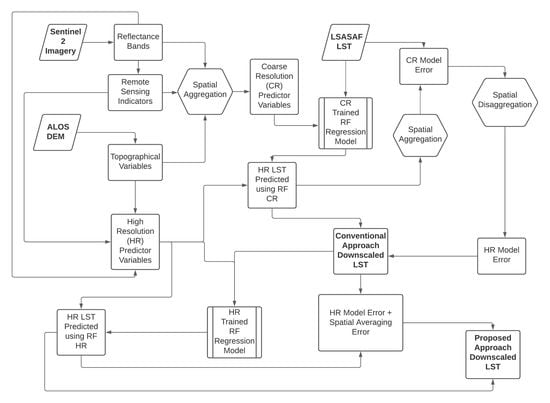
2.1.1. Proposed Downscaling Approach

The conventional approach of downscaling LST in RF is represented by the steps described by Equations (1)–(4). This approach has been widely adopted in various LST downscaling studies (e.g., [21,22,23,24]). The studies differ mainly in terms of the chosen predictor variables and the target coarse-resolution LST product.
The proposed approach follows the steps of the conventional approach from Equations (1)–(4). On the other hand, Equations (5)–(9) describe the extension of the conventional approach of downscaling LST in RF to derive the proposed improved approach for downscaling LST using RF regression.
In the first step, an RF regression linking model is trained using the coarse resolution LSA-SAF LST and predictor variables derived from Sentinel 2 and ALOS DEM. The linking model is defined using Equation (1) and describes the relationship between the predictor variables and the target LST at the coarse-scale.
L S T C R = F ( V a r _ C R i ,   V a r _ C R n )
where, L S T C R is the coarse resolution LSA-SAF LST, F is the linking model at the coarse resolution, V a r _ C R is the predictor variable aggregated to the resolution of the LSA-SAF LST, while i and n denotes the ith and nth selected predictor variable, respectively.
The linking model developed in Equation (1) is scene dependent, but the relationship it describes is assumed to be valid across multiple spatial scales within the scene, thus for each scene, a new model should be trained. Based on this assumption, the linking model is applied to the predictor variables at the fine spatial resolution to predict LST at the fine spatial resolution using Equation (2).
L S T F H R = F ( V a r _ H R i ,   V a r _ H R n )
where L S T F H R is the high-resolution LST modeled using the coarse resolution model   F , and V a r _ H R is the predictor variable at the fine spatial resolution.
However, since the selected predictor variables cannot fully account for all the variations in LST, the linking model has an inherent error; thus, the derived high-resolution LST should be corrected for this error. The model error correction procedure involves a spatial aggregation of the modeled high-resolution LST to the coarse resolution and subsequently computing the model error ( L S T C R ) as the difference between the original coarse resolution LSA-SAF LST and the aggregated LST from the model, as shown in Equation (3).
L S T C R   =   L S T C R   L S T F H R ¯
where L S T F H R ¯ is the predicted LST from Equation (2) aggregated to the coarse resolution. Prior to aggregation to the coarse scale, the high-resolution LST was first converted to radiance using the Stefan–Boltzmann law. Subsequently, the high-resolution radiance was aggregated to the coarse resolution and then converted to the aggregated LST at the coarse resolution by inverting the Stefan–Boltzmann equation. The emissivity used in the Stefan–Boltzmann equation was derived from fractional vegetation cover using the method of Jimenez-Munoz et al. [32]. The fractional vegetation cover was derived from the Normalized Difference Vegetation Index (NDVI) using the method of Carlson and Ripley [33]. The bare soil and full vegetation cover emissivity values adopted in the vegetation fraction based emissivity method are 0.97 Sobrino et al. [34], and 0.99 Sobrino et al. [35], respectively. This step was included in the aggregation procedure to avoid introducing biases in the aggregated LST owing to the non-linear relationship between radiance and LST.
In the model error correction step, it is assumed that the contribution to the model error by the fine resolution pixels that constitute the coarse resolution pixel is constant. Based on this assumption, the model error is resampled to the original resolution of the predictor variables and added to the high-resolution LST obtained using Equation (2) to derive the final downscaled LST as shown in Equation (4).
L S T H R   =   L S T F H R +   L S T H R
where L S T H R is the final downscaled LST based on the conventional approach, and L S T H R is the disaggregated model error.
However, in spatially heterogeneous environments and in particular, where the difference in spatial scales between the fine resolution predictor variables and the coarse resolution LST is large, this assumption is rarely satisfied.
The other shortcoming in the downscaling approach, especially when regression tree-based machine-learning algorithms such as RF are applied, is the assumption that the model developed in Equation (1) is valid across multiple spatial scales. The training data used to derive the model at the coarse-scale is an average representation of the spatial variability within the scene. Thus, as the difference in spatial scales between the fine resolution predictor variables and the coarse resolution LST increases, more spatial details which were not present at the coarse-scale will emerge. Since regression tree-based machine-learning algorithms are poor at predicting data outside the range of data present during training, the model trained at the coarse resolution will rarely capture such spatial details.
To counter this problem, the high-resolution LST obtained in Equation (4) is used to construct a new RF regression model and predict new data range-enhanced LST at the fine resolution using Equation (5).
L S T f H R   =   f ( V a r _ H R i ,   V a r _ H R n )
where L S T f H R is the data range enhanced high-resolution LST, and f is the RF regression model trained at the fine resolution.
Unlike the LST predicted using Equation (2), the LST from Equation (5) is less affected by issues related to averaged data ranges in the training data. However, the LST from Equation (5) still needs to be corrected for the model error, since the selected predictor variables cannot entirely account for the variations in LST. Also, it should be adjusted for the averaging effect related to the constant redistribution of the model error in the fine resolution LST obtained using Equation (4). Thus, the final corrected LST is represented by Equation (6).
L S T N H R   =   L S T f H R +   L S T H R + L S T A V G
where L S T N H R is the final downscaled LST using the proposed approach and L S T A V G is the averaging effect in the model error correction procedure.
The difference between the LST from Equation (4) and LST from Equation (5) is assumed to be primarily related to the averaging effect in the model error correction procedure. Thus, the averaging effect can be approximated using Equation (7).
L S T A V G   =   L S T f H R L S T H R
Substituting Equation (4) into Equation (7) and rearranging the terms yields:
L S T H R + L S T A V G   =   L S T f H R L S T F H R
Equation (8) indicates that the corrections for the model error and the averaging errors can be approximated as the difference between the LST predicted using Equation (5), and LST predicted using Equation (2). Thus, Equation (6) can be rewritten as follows:
L S T N H R   =   2 × L S T f H R L S T F H R
Equation (9) represents the final proposed approach for downscaling LST in complex environments using RF regression.
Besides enhancing the spatial details in the LST predicted at the fine resolution, the proposed approach indirectly incorporates the coarse-resolution model error correction as shown in Equation (8). Thus, the impact of the coarse-resolution model error correction on the downscaled LST should be less pronounced since the approach does not assume a constant redistribution of the coarse-resolution model error.
Due to the indirect incorporation of the model error correction as opposed to the direct addition of the model error in the conventional method (Equation (4)), the proposed approach will also predict LST even for cloud-contaminated pixels during the overpass time of the thermal sensor. However, the LST predicted for the cloud contaminated pixels will be highly uncertain since the RF regression models used to derive L S T f H R and L S T F H R do not contain any information on LST under cloudy conditions. Thus, we strongly recommend masking out the cloud-contaminated pixels using the cloud mask of the thermal image.

2.1.2. Random Forest Model Description

Random forests [27] are an ensemble decision tree-based supervised machine learning algorithm. The ensemble consists of an average over several randomized and de-correlated decision trees adapted for either classification or regression. For regression purposes, non-linear multivariate regression trees are constructed, with a set of decision rules being used to determine the splitting when building the trees. A bootstrap sample which contains about two-thirds of the observations is selected during model training to grow each tree, and by using a randomly selected subset of predictors, the chance of model overfitting is reduced. Splits are achieved by minimizing a cost function between the target and the predictors resulting in a regression tree.
A third of the unseen observations during model training are used to compute the popular out-of-bag (OOB) error estimate in RF [27]. A prediction is constructed for each of the unseen data instances using only those regression trees in which the respective data instance was not used in training. The average error over all OOB predictions is then used to derive the overall OOB score, providing a convenient way of assessing the performance of the model. On the other hand, improvements recorded on the splitting decision at each split node and for each tree are used to derive variable importance rankings, enabling the assessment of the contribution of each predictor to the final model. Other advantages include the ability of RF to account for correlations among features [29,36], to handle continuous and categorical data simultaneously, and the relatively small number of model parameters needed [37].
In this study, the RF regression framework for the downscaling of LST was implemented in Python using the scikit-learn (sklearn) package [38].

2.1.3. Selection of Predictor Variables

Multiple predictors are often needed to adequately describe variations in LST in fragmented landscapes owing to the complex interactions between LST and various factors related to climate, land use and land cover (LULC), and topography [22]. However, besides the computation demand that comes with increasing the number of predictors in machine-learning algorithms, it has been shown that an increase in the number of predictors increases the risk of model overfitting [39]. Additionally, despite the ability of RF to handle high-dimensional and correlated variables, it has been shown that high-dimensional variables can lead to inflated OOB accuracy scores and model instability [40].
Given these shortcomings, an objective feature selection approach based on the recursive feature elimination with cross-validation (RFECV) implemented through the sklearn package was chosen for selecting predictor variables. RFECV is a combination of the iterative feature elimination criterion proposed by Guyon et al. [39] and a cross-validation (CV) data splitting strategy. The iterative feature elimination involves the removal of the least ranked feature at each step based on weights computed based on a minimization objective function. In this study, an RFECV with the mean squared error (MSE) as the objective function and a CV of 3 (default in sklearn) was adopted. The predictors selected through the RFECV criterion were then used to train the RF regression linking model.

2.1.4. Validation of Downscaled Land Surface Temperature (LST) Maps

Owing to the scarcity of in situ LST measurements, checking for product consistency against results obtained from other models or LST products is a generally accepted indirect validation approach in LST-related studies [1,41]. As such, per pixel comparison between LST maps derived through downscaling and LST maps derived from Landsat 8 was performed to check for consistency between the downscaled LST against the one derived from Landsat 8. The performance of the downscaling approaches was evaluated in terms of the root mean squared error (RMSE), the coefficient of determination (R2) and bias, described by Equations (10)–(12), respectively.
R M S E =   1 n i = 1 n ( L S T m L S T r ) 2
where L S T m is the modeled LST, L S T r is the reference LST and n is the total number of pixels.
R 2 = 1   ( L S T r L S T m ) 2 ( L S T r L S T r ¯ ) 2
where L S T r ¯ is the mean reference LST.
B i a s =   i = 1 n ( L S T m L S T r ) n

2.2. Study Area and Data
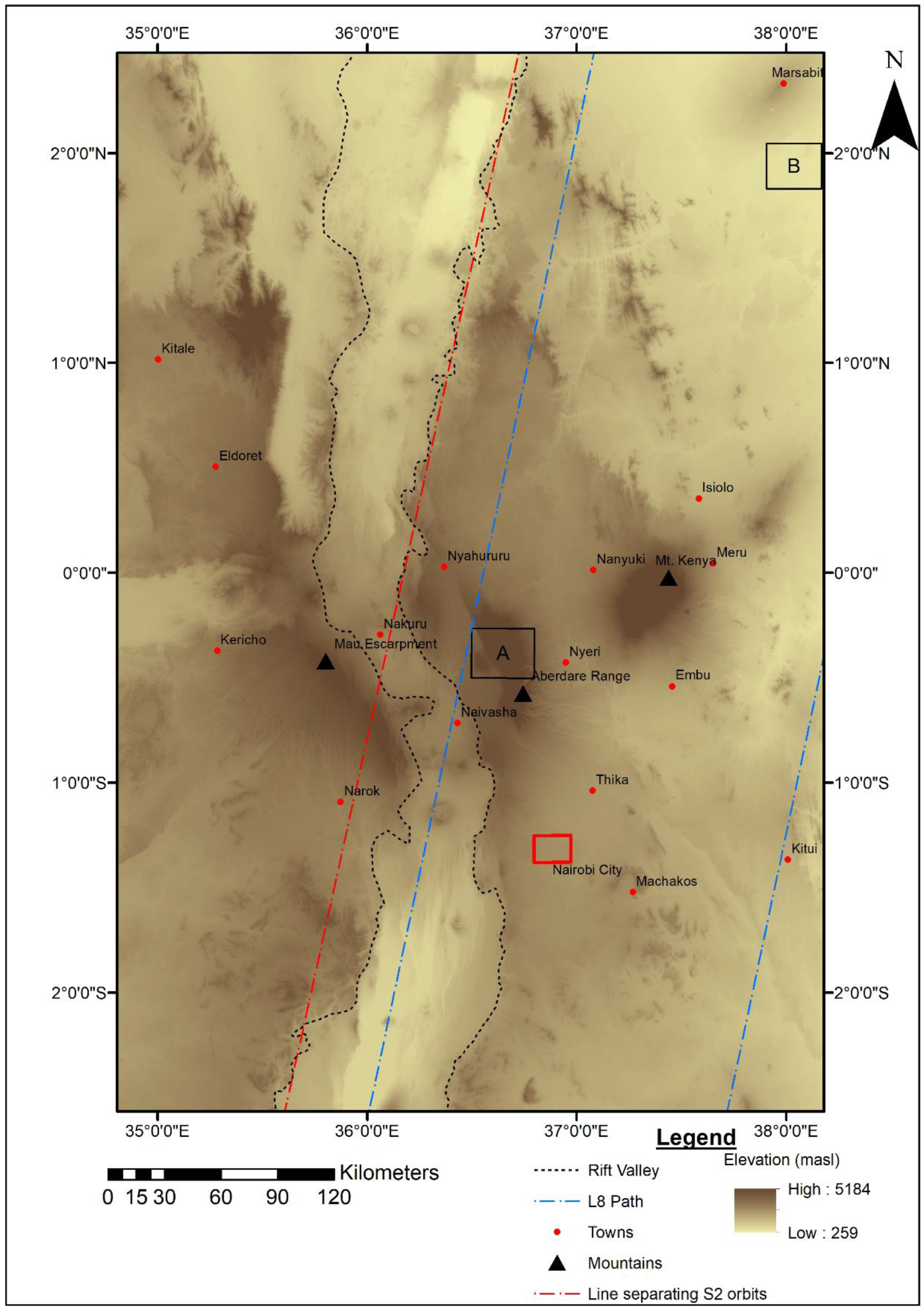
2.2.1. Study Area

The study area is located in Kenya and lies roughly between 35°E and 38°E, and 3°S and 3°N as shown in Figure 1. The study area coverage was influenced mainly by the availability of coinciding orbital paths for both Sentinel 2 and Landsat 8. The red dotted line in Figure 1 indicates the separation between the two orbital paths of Sentinel 2, 092 to the right, and 135 to the left, which makes up a mosaic of the study area. On the other hand, the orbital path for Landsat 8 in Figure 1 corresponds to orbital path number 168, and is a mosaic of tile numbers 059, 060 and 061, and forms the validation area for the downscaling. Although the orbital path of Landsat 8 falls exclusively on orbital path 092 of Sentinel 2, the study area was extended to cover path 135 to increase the thermal contrast within the study area. Since the time lag between the overpass dates for path 092 and 135 is three days at maximum, it was assumed that no significant discrepancies would arise on the reflectance mosaic obtained from the two orbits. The total study area consists of a mosaic of approximately 24 full tiles of Sentinel 2.
The study area is characterized by pronounced topographical differences with elevation ranging from as low as 259 m above sea level (masl) in the northern parts to as high as roughly 5184 masl on top of Mt. Kenya. The study area is straddled from north to south by the eastern branch (Kenyan Rift valley system) of the East African Rift System (EARS). The Kenyan Rift Valley system cuts in between the Mau Escarpment and the Aberdares Mountain Ranges at the central part of the study area, creating areas with sharp elevation drop between the mountains and the floor of the valley. Variations in climatic conditions within the study area are mainly topography-induced. Mean daily air temperature range from less than 10 °C in the mountains to above 30 °C in the low lying ASAL regions. The study area is also characterized by highly fragmented LULC due to the highly mixed land use related to small scale farming activities.

2.2.2. Data Acquisition and Processing

Table 1 shows the datasets used in this study, their characteristics, and their respective sources.
The LSA-SAF LST product [42] was used as the coarse target resolution LST for building the model. The LST product from LSA-SAF is an operational LST product disseminated through the Satellite Application Facility on Land Surface Analysis (Land-SAF) of the European Organization for the Exploitation of Meteorological Satellites (EUMETSAT) in near real-time at time intervals of 15 min and at a spatial resolution of approximately 3 km at sub-satellite. It is derived from the split window channels of the SEVIRI sensor onboard the MSG suite of weather satellites based on the generalized split-window algorithm proposed by Dozier, [43] adopted for the SEVIRI sensor [42,44]. The product has consistently been shown to meet the set target RMSE of 2 K [45,46].
The ALOS World 3D-30m (AW3D30) DEM [47], was used to derive topography-related predictors, namely Elevation, Slope, and Aspect. ALOS DEM is considered the most accurate of the current freely available DEM’s averaging an RMSE of 1.78 m for the vertical height [48]. The ALOS DEM-derived predictor variables were then aggregated to the sampling resolution (100 m) of Landsat 8 TIR bands, which was adopted as the base resolution for the downscaling model in order to match the spatial resolution of the validation LST maps derived from Landsat 8.
Sentinel 2 Level 1C products represent the top of atmosphere (TOA) reflectance and were downloaded and converted to surface or bottom of atmosphere (BOA) reflectance by correcting for atmospheric effects using the Sen2Cor algorithm [49]. A total of 11 bands were obtained after atmospheric correction since the coastal aerosol, and the cirrus bands do not contain surface information, thus not included as part of the Level 2A product produced by the Sentinel Application Platform (SNAP) software. The bands obtained after atmospheric correction include Blue, Green, Red, Near Infrared (NIR), Red Edge 1 (RE1), Red Edge 2 (RE2), Red Edge 3 (RE3), Narrow Near Infrared (NNIR), Shortwave Infrared 1 (SWIR1), Shortwave Infrared 2 (SWIR2), and the Water vapor (wvp band). The cloud and cloud shadow masks produced during the atmospheric correction procedure were applied to the remaining surface reflectance bands to obtain cloud-free pixels. Cloud-free pixels from two consecutive overpasses were then used to create composite images, with reduced effects of cloud contamination. The dates for the Sentinel 2 images used to generate the composite images, the LSASAF LST acquisition dates, and the corresponding Landsat 8 overpasses are shown in Table 2.
The composite surface reflectance images were then resampled and co-registered to match the sampling spatial resolution (100 m) of Landsat 8 TIR bands. The resampled surface reflectance bands were then used directly as predictor variables. Additionally, the surface reflectance bands were used to derive the additional remote sensing predictor variables shown in Table 3.
Landsat 8 imagery and Total Column Water Vapour (TCW) product from the European Centre for Medium-Range Weather Forecasts (ECMWF) reanalysis (ERA-5) were used to derive LST maps for validating the downscaled LST maps. Landsat 8 LST maps were derived based on the generalized split-window algorithm proposed by Li and Jiang, [41] for Landsat 8 data. Before the derivation of the LST maps from Landsat 8, all the datasets were resampled to the sampling resolution (100 m) of Landsat 8′s TIR bands. It should be noted that, although stray light contamination had plagued the TIR bands of Landsat 8 [50], an operational stray light correction procedure was implemented in 2017 to correct for these artifacts [51]. Gerace and Montanaro, [51] report that the fidelity of the corrected bands is within the range of that of MODIS TIR channels. Li and Jiang, [41] reported an error of less than 1 K using their generalized split-window algorithm in comparison to the MOD11_L2 V6 MODIS LST product, indicating the ability of the algorithm to retrieve LST from the TIR bands of Landsat 8 accurately.
Table 3. Sentinel 2-derived remote-sensing indicators.
Remote Sensing IndicatorTargeted Surface/CharacteristicsFormulationAuthor
Normalized Difference Vegetation Index (NDVI)Vegetation ( NIR Red ) ( NIR + Red ) [52]
Enhanced Vegetation Index (EVI)Vegetation 2.5 × ( NIR Red ) ( NIR + 6 × Red 7.5 × Blue + 1 ) [53]
Soil-Adjusted Vegetation
Index (SAVI)
Vegetation ( NIR Red ) ( NIR + Red + 0.5 ) × ( 1 + 0.5 ) [54]
Fraction Vegetation Cover (FVC)Vegetation cover/density ( ( NDVI NDVI s ( NDVI v NDVI s ) ) 2 Where NDVI v = 0.86 and NDVI s = 0.20 [33,55]
Bare Soil Index (BSI)Bare soil surfaces ( SWIR 1 + Red ) ( NIR + Blue ) ( SWIR 1 + Red ) + ( NIR + Blue ) [56]
Normalized Difference Built-up Index (NDBI)Built-up areas SWIR 1 NIR SWIR 1 + NIR [57]
Normalized Difference Water Index (NDWI)Water bodies ( Green NIR ) ( Green + NIR ) [58]
Normalized Multi-band Drought Index (NMDI)Soil and Vegetation moisture stress NIR ( SWIR 1 SWIR 2 ) NIR + ( SWIR 1 SWIR 2 ) [59]
Normalized Difference Water (Moisture) Index (NDMI)Vegetation Water Content ( NIR SWIR 1 ) ( NIR + SWIR 1 ) [60]

3. Results

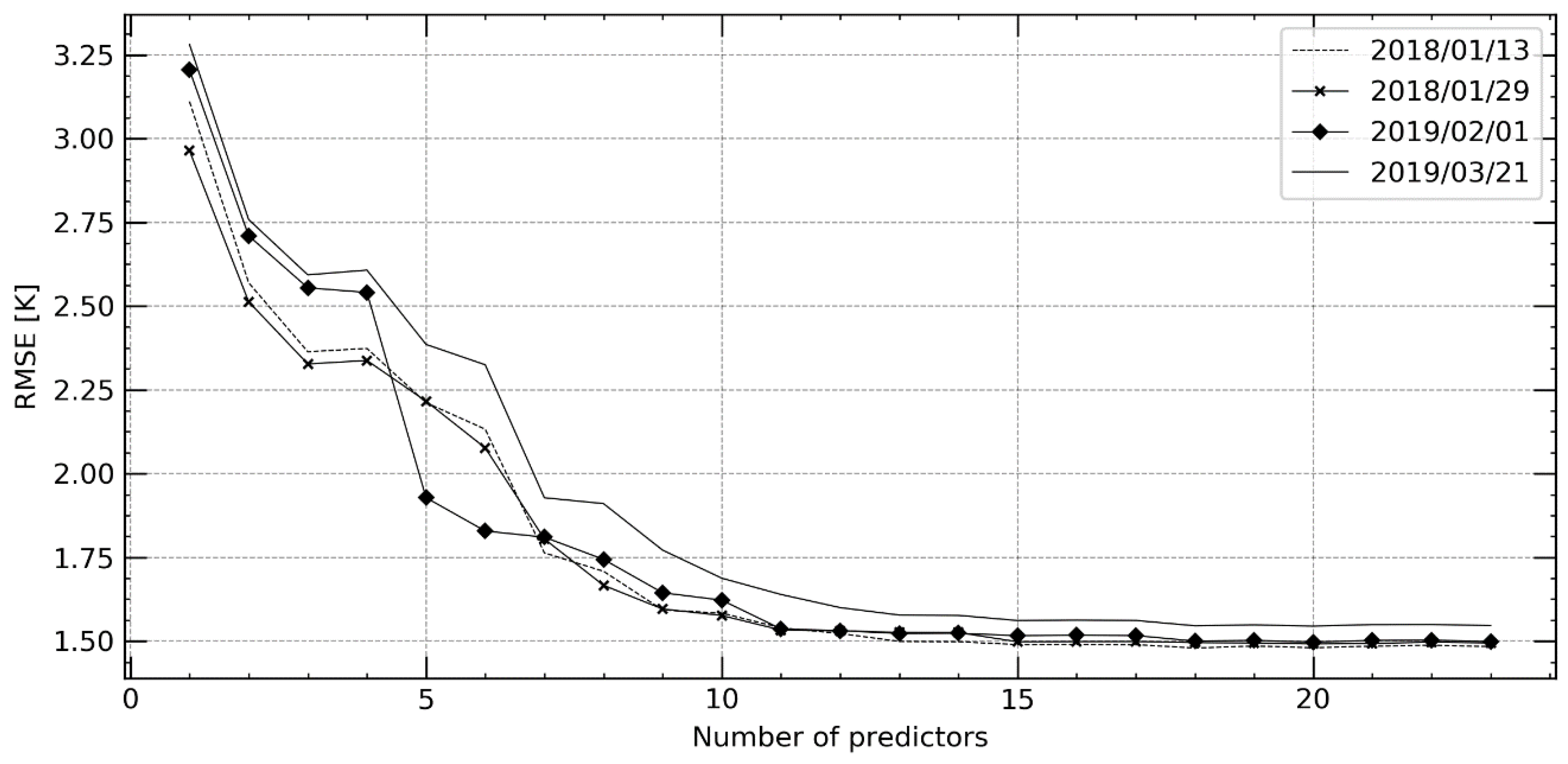
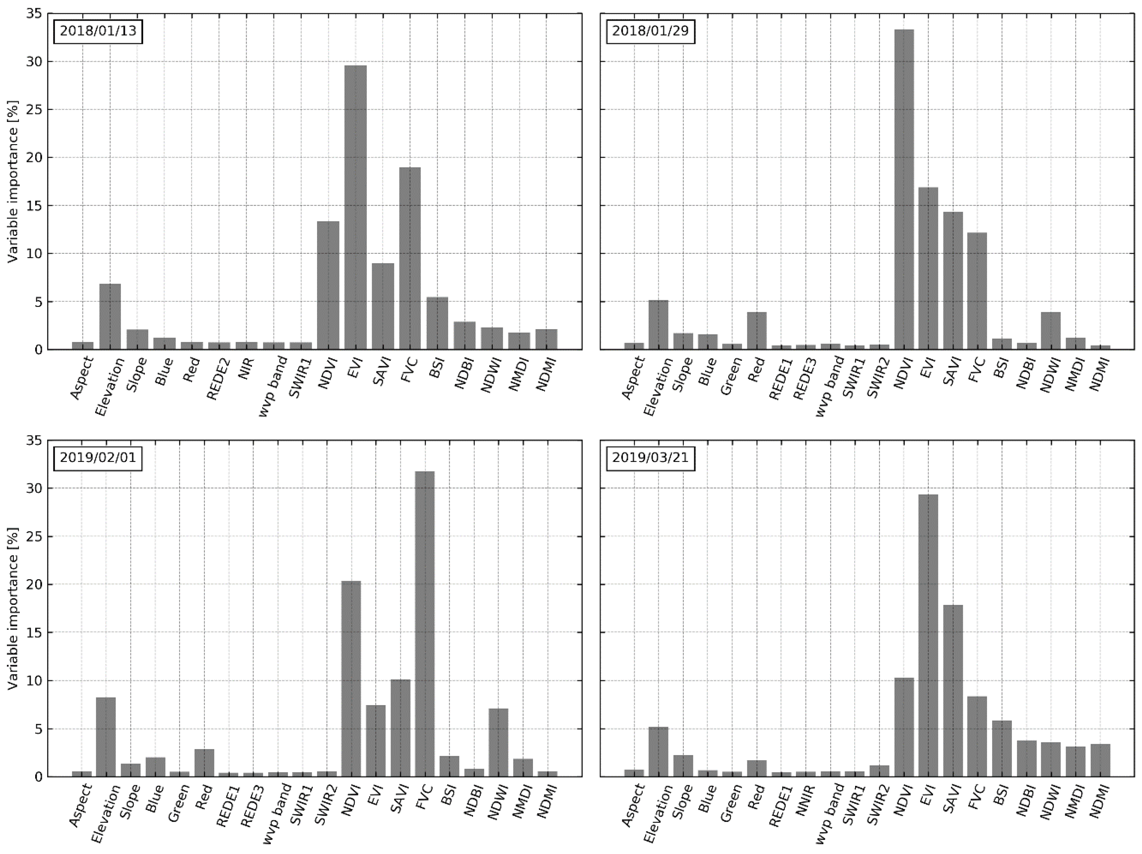
3.1. Selection of Predictor Variables

The results of the predictor variable selection process are shown in Figure 2 and Table 4. Figure 2 shows the influence of increasing the number of predictor variables on the model’s performance. The model performance increases drastically when predictor variables are increased from 1 to about 12 variables, as indicated by the decrease in the RMSE with increasing variables. Beyond 12 variables, increasing the number of variables yields minimal effect on the model performance.
Table 4 shows the total number of variables selected, the RMSE values obtained during the variable selection process using RFECV, and the OOB score values for models trained using all the variables and the RFECV selected variables, respectively. In three of the four days, RFECV variable selection resulted in 20 variables except for 13 January 2018, when 18 variables were selected. Overall, the performance of the models based on the two sets of predictor variables is more or less the same.
Figure 3 shows the individual variables selected through RFECV for each day and their respective percentage contribution to the final model. Although the RFECV variable selection did not show much variation in the number of selected variables across the days considered, the individual variables selected vary across the days, as observed in Figure 3. Topography-related variables and indices are constantly selected, and only reflectance variables change during the selection process across the four days. In terms of the contribution of the variables to the final model, vegetation indices, i.e., NDVI, Enhanced Vegetation Index (EVI), Soil-Adjusted Vegetation Index (SAVI), and the Fraction Vegetation Cover (FVC), have the highest contribution to the final model. The least contribution is observed in reflectance variables. Elevation follows the vegetation-related indices in the contribution to the final model. From Figure 3, it is also observed that the overall trend in terms of the percentage contribution by the topography-related variables is mostly unchanged.

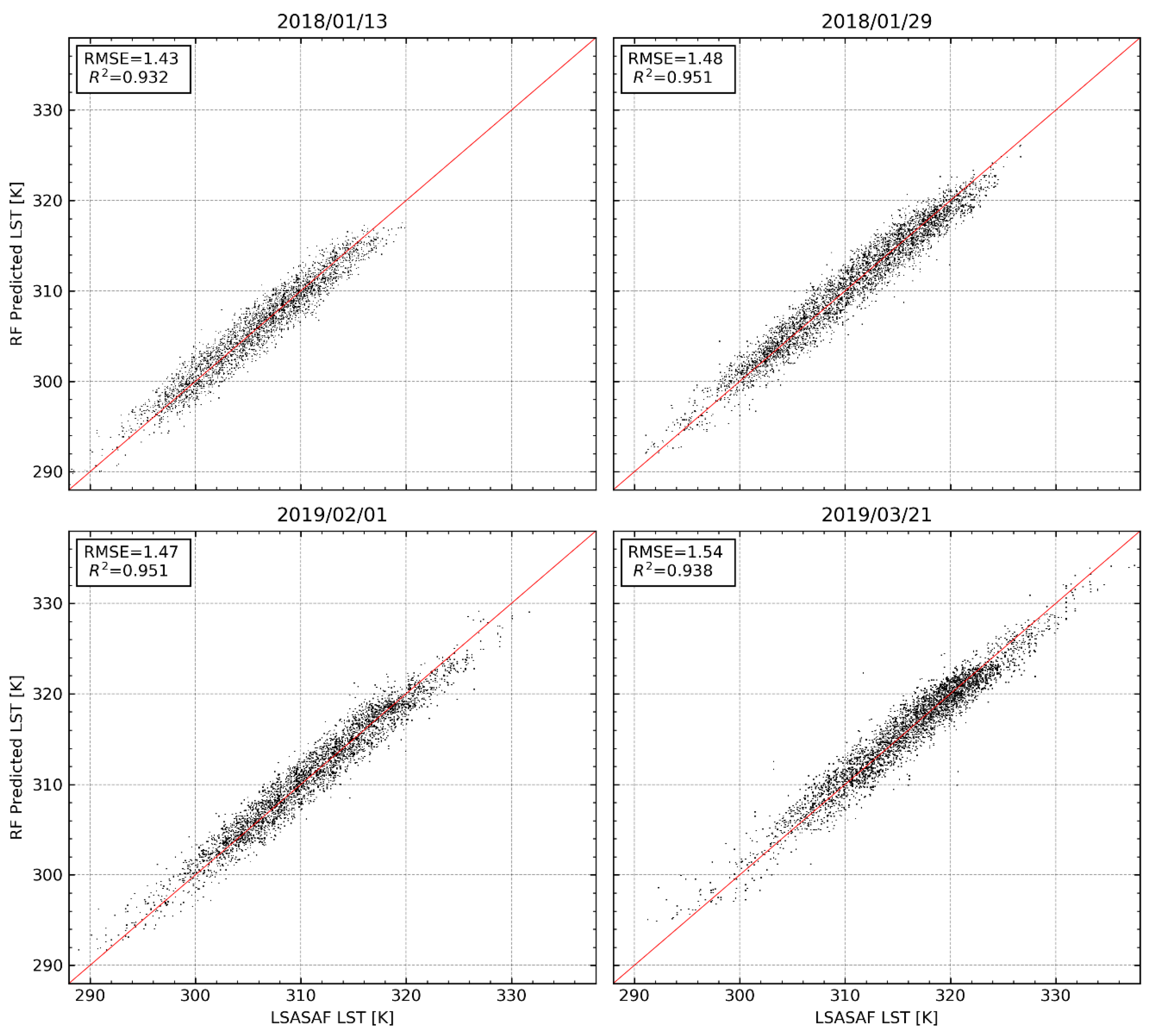
3.2. The Prediction Ability of the Selected Model

Figure 4 shows the scatterplot between the original LSA-SAF LST and the predicted LST obtained using the RF regression model built on the selected variables at the coarse-scale, with the data split into 70% to 30% training and validation sets, respectively. The spread between the points is quite linear and follows the one-to-one line.
To investigate the ability of the developed model to predict LST at high resolutions, LST predicted by the model was compared to LST derived from Landsat 8. The results of the comparison are shown in Figure 5. The results indicate a linear relationship between the predicted LST and Landsat 8 LST. However, compared to results at the coarse scale (Figure 4), a decrease in the model performance is observed in Figure 5. There is a reduction in the model performance both in terms of the R2 and the RMSE. Notably, a significant departure from the linear trend is observed in both the upper and lower limits of the scatterplots. At the lower limits, Landsat 8 LST decreases without a corresponding decrease in the predicted LST. In contrast, at the upper limits, Landsat 8 LST increases without a corresponding increase in the predicted LST. Although the model performance at the high resolution is considerably lower, the trend in the model performance in terms of both the R2 and the RMSE observed in Figure 5 is consistent with the trend in the model performance seen in Figure 4.

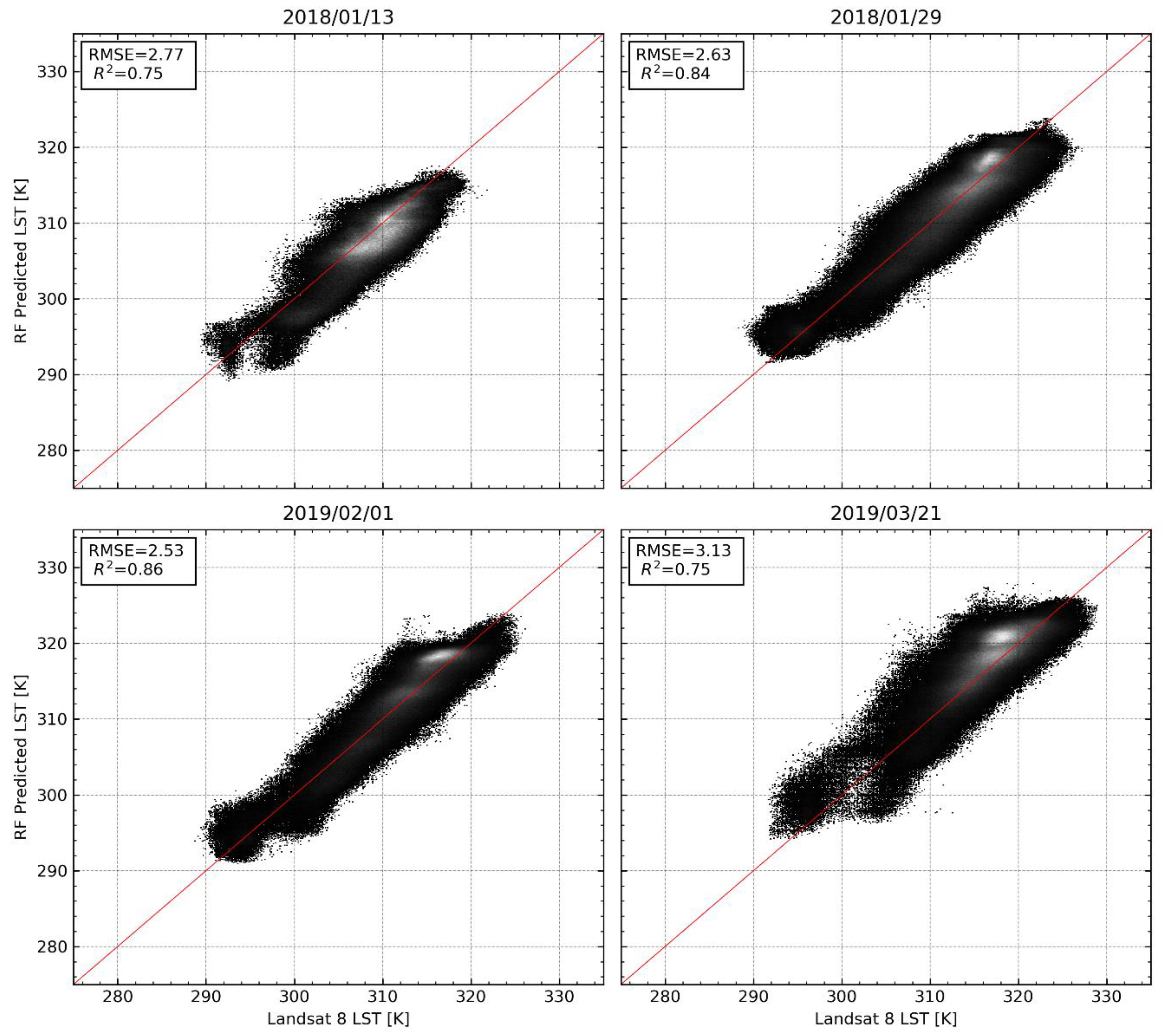
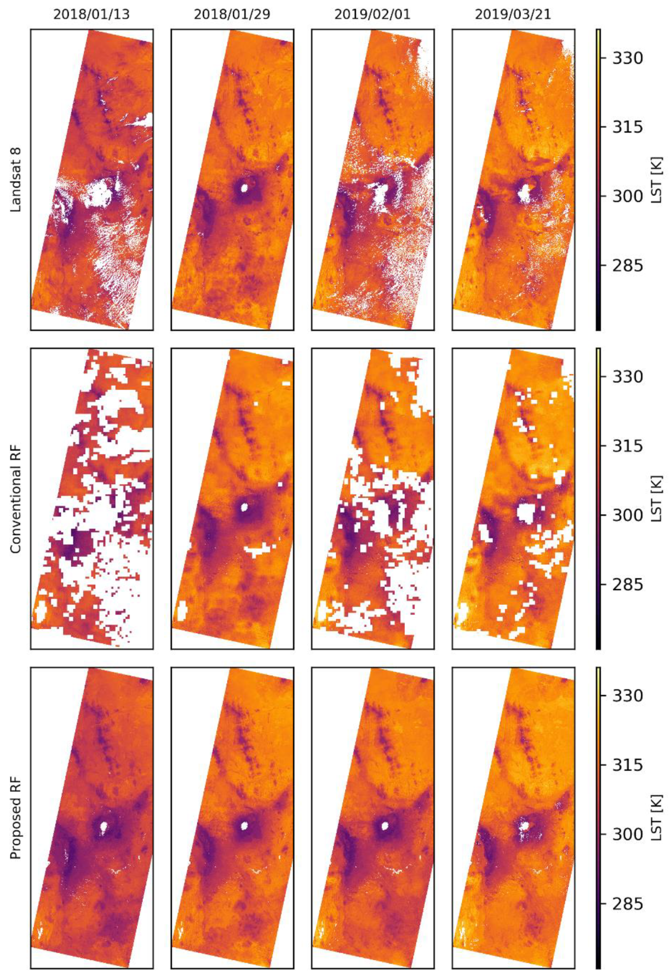
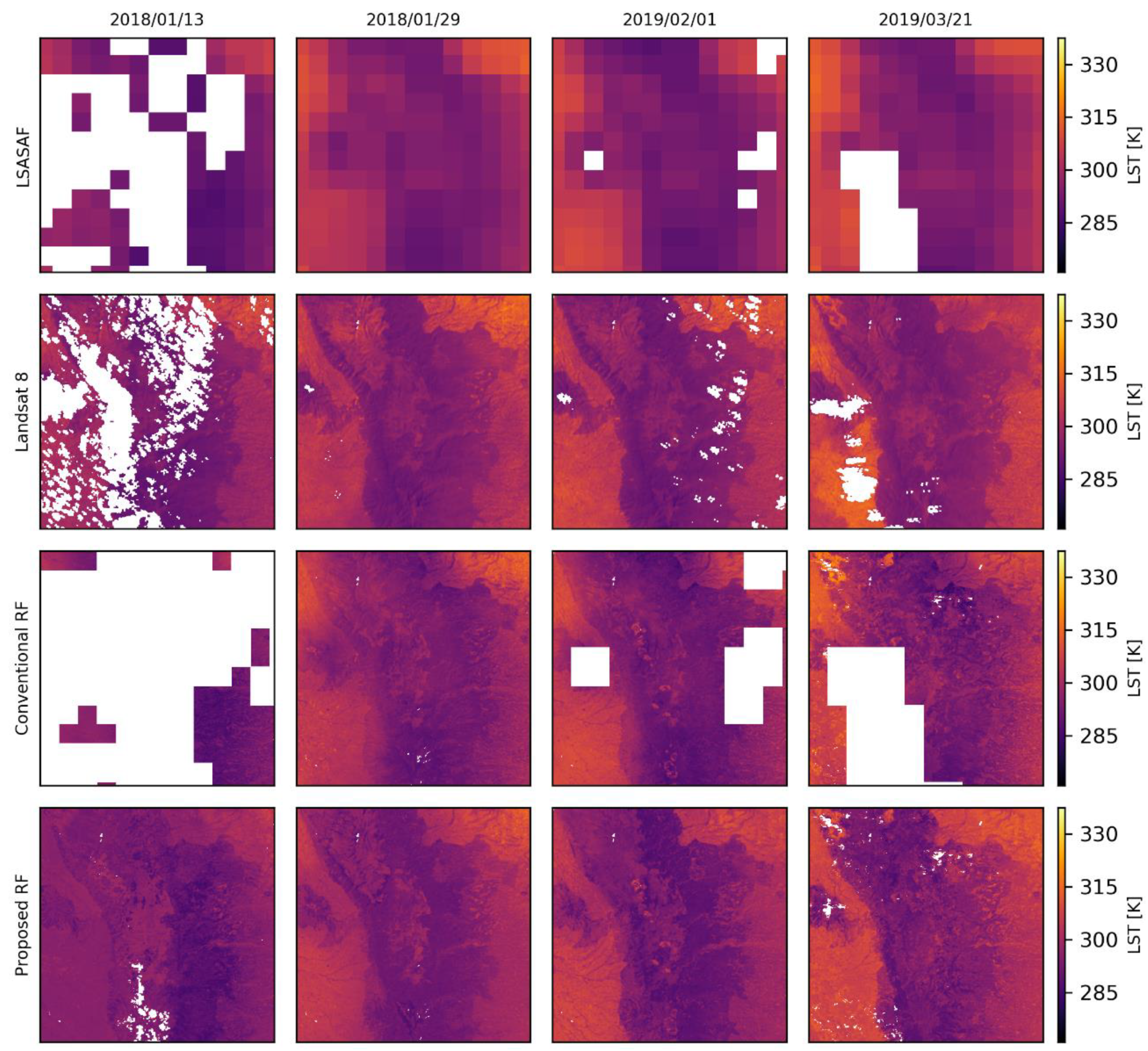
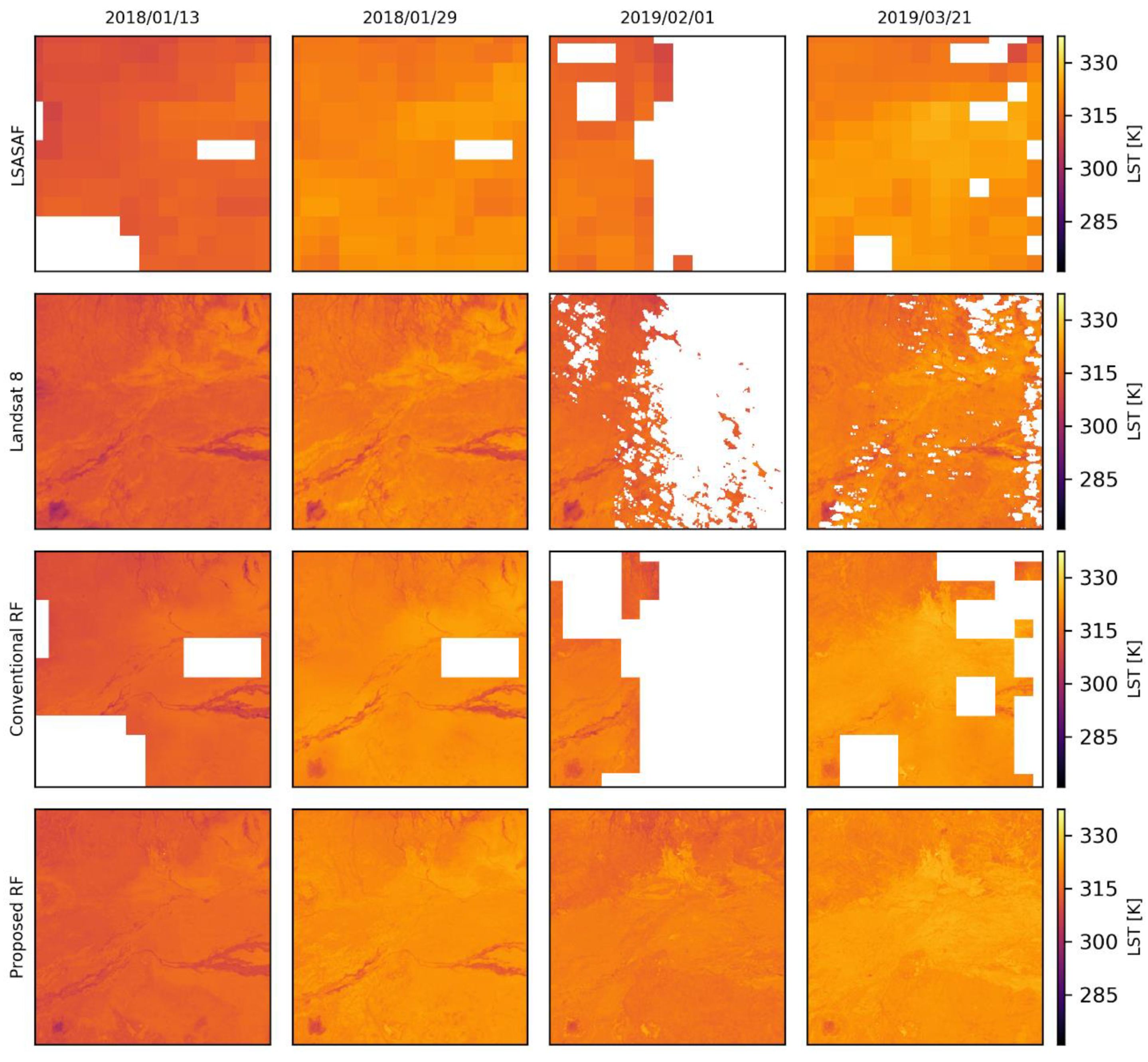
3.3. Downscaling Results

Figure 6 shows LST maps derived from Landsat 8 and the downscaled LST maps obtained using the conventional RF approach and the proposed RF approach. The downscaled LST maps from both approaches show consistency with Landsat 8-derived LST maps both in terms of the spatial details and variations in the LST across the four days. One notable difference is the considerably lower amount of pixels with missing data (white patches) in the maps derived using the proposed approach in comparison to the maps obtained using the conventional approach as well as from Landsat 8. The pixels with missing data are mainly related to cloud cover, and to a lesser extent, water bodies.
Figure 7 shows LST maps for a section of the Aberdares Mountain ranges, one of the areas in the study area that is characterized by complex terrain. The downscaled LST maps in Figure 7 show more spatial details than the coarse-scale LSA-SAF LST maps. The spatial details in the downscaled maps are also consistent with the ones observed in the Landsat 8 LST maps. However, the maps obtained using the proposed approach show enhanced details, which are more consistent with the ones observed in the Landsat 8 LST maps, especially in the transition zones between the mountains and the surrounding areas.
Figure 8 shows an ASAL area in the semi-arid northern part of Kenya. Similar to the observations in Figure 7, enhanced spatial details are observed in the downscaled images in comparison to the LSA-SAF LST maps. In addition, more spatial details and better spatial consistency with Landsat 8 LST maps are observed in the maps derived using the proposed approach than in the conventional approach. However, it is also observed that the downscaled maps from both approaches show slightly higher LST than that observed in the Landsat 8 LST maps.
Figure 9 shows the linear regression results between the Landsat 8 derived LST and the downscaled LST from the two approaches. The regression results confirm the spatial consistency observed between Landsat 8 LST maps and downscaled LST maps in Figure 6. A strong linear relationship is observed between the Landsat 8 LST and the downscaled LST using both downscaling approaches. However, the proposed approach shows a slightly better performance in terms of the R2 in comparison to the conventional approach on 29 January 2018 and 1 February 2019 while a slight deterioration in the R2 is observed on 13 January 2018 and 21 March 2019. In terms of the RMSE, the proposed approach performs marginally better than the conventional approach across all the days. In terms of the bias, the proposed approach shows a better performance than the conventional approach across all the days apart from 13 January 2018. With regards to the spread of points relative to the one-to-one line, the proposed approach shows less scatter, especially at the lower temperatures. However, the proposed approach shows more scatter in the upper-temperature ranges in some of the days, e.g., on 21 March 2019. Based on the scatterplots, it is also evident that, in general, both downscaling approaches tend to overestimate the LST observed by Landsat 8 at the higher LST values.
Table 5 shows the statistical results for three categories of vegetation cover classified based on NDVI ranges.
Based on the statistical results presented in Table 5, the least performance based on the conventional approach is observed in the fully vegetated areas. In contrast, the best performance based on the conventional approach is observed in the sparsely vegetated areas. The proposed approach shows a significant improvement in the performance of the downscaled LST in partial and full vegetation canopies based on both the R2 and the RMSE in comparison to the conventional approach. In terms of the R2, an average increase of 0.07 and 0.22 is observed in the partially and fully vegetated areas, respectively. In terms of the RMSE, an average reduction of 0.99 and 1.32 K is obtained in the partially and fully vegetated areas, respectively. However, in the sparsely vegetated areas, the proposed approach shows a slight deterioration. An average reduction of 0.06 in the R2 and an increase of 0.02 K in the RMSE is observed in the sparsely vegetated areas. The proposed approach shows a lower bias across the three classes of vegetation coverage in comparison to the conventional approach. Based on the bias, it is also observed that both approaches overestimate the Landsat 8 LST in the sparsely vegetated areas and underestimate Landsat 8 LST in both the partially and fully vegetated areas.

4. Discussion

The main goal of this study was to reduce the spatial averaging bias inherent in LST downscaling methodology using RF regression in complex environments. As noted in Kustas and Anderson, [2], in complex environments, the partitioning of available energy at the land surface is influenced by many other factors besides soil moisture and vegetation cover. Thus, as highlighted in Hutengs and Vohland, [22], Yang et al. [24] and Zhao et al. [25], additional predictor variables, especially those that have an influence on albedo, surface emissivity, and solar insolation are vital for downscaling LST in complex environments. The results shown in Figure 2 are a confirmation of the added benefits of using multiple predictors variables in the downscaling of LST in complex environments. However, based on the results in Figure 2 and Table 4, it is evident that there is a limit to the number of predictor variables that are beneficial to the model performance. As observed in Figure 2, it appears that the inflection point in terms of the contribution of the predictor variables to the model performance is about 12 variables. Thus, most of the predictor variables beyond the inflection point are likely redundant. The redundancy may likely be due to correlated predictor variables or simply because some predictor variables have little correlation with LST. Although RF is not highly affected by feature correlation, it is beneficial to carry out variable selection since, as pointed out in Guyon et al. [39] and Millard and Richardson, [40], besides reducing the computation demand, the choice of predictors in machine learning reduces the dimensionality problem and thus lowers the risk of model overfitting. Based on the results presented in Figure 3, it appears that reflectance bands constitute most of the redundant predictors. They are the most affected during the process of variable selection in RFECV, and in most cases, have the least contribution to the final model, indicating that they are weaker LST predictors. Similar findings have been reported in Yang et al. [24] and are attributed to the fact that, unlike remote-sensing indices, raw reflectance bands contain less information on the characteristics of the surface. The high contribution by vegetation indices to the linking model observed in Figure 3 is an assertion to the well-established LST-VI feature space concept reported in Sandholt et al. [16]. On the other hand, the stable contribution by topography-related variables shows the significant influence of topography on LST in complex terrain and agrees with findings in Hutengs and Vohland, [22] and Zhao et al. [25].
Although the risk of overfitting in RF is low even in the presence of correlated variables [27,29,36], Strobl et al. [29] note that correlation has huge influence on the variable importance measures generated using RF. The considerable variations in each vegetation index’s contributions despite their relatively constant combined contribution to the final model observed in Figure 3 across the four days support the argument by Strobl et al. [29]. Through random selection of predictor variables, the effect of collinearity on the prediction ability of RF is reduced since the contribution of the other correlated variables is significantly reduced because the impurity they can remove is already removed by the first randomly selected predictor variable. Besides, as noted in Strobl et al. [29], the random selection of predictor variables allows for the inclusion of marginalized predictors in the ensemble, thus improving the stability of the model. However, since the random permutation importance approach employed in the computation of variable importance in RF assesses the change in the model performance based on the presence or absence of the selected variable, collinear variables will tend to compensate for each other during the process of random permutation, leading to biases in the variable importance derived from RF. Thus, as observed in Figure 3 any of the correlated variables can be selected to remove the impurity when splitting the nodes making it difficult to determine the individual contribution of each predictor variable to the final model. Consequently, as argued in Matsuki et al. [36] the contribution of the correlated vegetation related variables in Figure 3 can only be interpreted as group and not independently.
Results presented in Figure 4 indicate that the linking models built using Equation (1) are capable of predicting LST in each of the respective model training scenes. A high linear relationship exists between the modeled LST against the 30% unseen LST data set aside during model training, as confirmed by the high R2 (0.94 on average), indicating the selected predictors can largely explain the thermal variability in the respective scenes. However, upon transfer to the fine spatial resolution, the model performance deteriorates. This deterioration is primarily due to the inability of the selected predictor variables to account for other variations in LST at fine resolution [17]. However, the trend observed on the extreme edges of the scatterplots in Figure 5 cannot be attributed solely to the inability of the predictor variables to capture variations in LST at high resolution. This trend is attributed to the inability of the RF model to predict beyond the data range present in the training data. This trend indicates that the model developed at the coarse-scale largely represents the average conditions within the scene, thus cannot adequately capture the variations in LST under extreme conditions.
Based on visual comparison of the downscaled LST maps presented in Figure 6, not much difference can be discerned between the conventional approach and the proposed approach, apart from less cloud contamination in the maps derived from the proposed approach. However, the zoomed-in areas shown in Figure 7 and Figure 8 indicate that besides lesser cloud contamination, more spatial details consistent with Landsat 8 LST maps are observed in the LST maps derived using the proposed approach. This improvement is attributed to the step implemented to enhance the data range in the RF regression model and the model error correction procedure adopted, which avoids a constant redistribution of the model error calculated at the coarse-scale. However, this step results in the proposed approach reproducing LST even under cloud-contaminated pixels, resulting in less cloud-contaminated LST maps. Although this might be appealing to the user, as suggested in the methodology, it is strongly recommended to mask out the cloud-contaminated pixels. As pointed out in Martins et al. [44], clouds alter the redistribution of the incoming shortwave and longwave radiation at the surface resulting in an entirely different energy balance at the surface in comparison to the energy balance under clear sky conditions. The relatively poor performance in terms of the spread of scatter points observed on 13 January 2018 in Figure 9 also suggests that cloud cover may influence the downscaling results since cloud masking may not detect all the cloud-contaminated pixels. Besides, as pointed out in Kustas et al. [17] and Hutengs and Vohland, [22], downscaling of LST is influenced considerably by thermal contrast within the scene, which may be affected by excessive cloud cover. The reduced thermal contrast may lead to an imbalance in the distribution of LST values in the target LST when training the model. As noted in Millard and Richardson [40], imbalances in the target variable will increase the risk of model overfitting, undermining the model’s prediction ability. However, the effect may also be related to the effect of cloud cover on Landsat 8 LST, since the coarse resolution, TCW product used cannot capture the high spatial variability in atmospheric water vapor under cloudy conditions.
The statistical results shown in Table 5 and the scatterplots in Figure 9 indicate that the proposed approach is superior to the conventional approach, especially in vegetated areas. Vegetated areas mainly correspond to the lower temperatures where much of the improvement in the scatter in Figure 9 is observed. The weaker performance in vegetated areas compared to the sparsely vegetated areas based on the conventional approach, appears to contradict results from other studies, e.g., in Kustas et al. [17] and Agam et al. [18]. However, the weaker performance is mainly attributed to topography since most of the fully vegetated areas correspond to forested areas in the mountains. In contrast, the sparsely vegetated areas are mostly located in low lying areas where the effect of topography is less pronounced. As pointed out in Hutengs and Vohland, [22], the complex terrain in mountainous areas has profound implications on LST downscaling. The significant improvement observed in the fully vegetated areas using the proposed approach can be attributed to an improved ability of the proposed approach to capture the spatial details in the complex mountain environment. The enhanced spatial details are due to reduced spatial averaging errors related to the coarse model and the model error correction in the proposed approach.
The biases observed in the downscaled LST in both approaches may be partly related to systematic differences in the Landsat 8 LST and the coarse-resolution LSA SAF LST. However, the tendency by the downscaled LST to overestimate the Landsat 8 LST in the arid sparsely vegetated areas may also be partly attributed to the inability of the selected predictor variables to capture the thermal variability related to other factors such as soil moisture. In addition, it should also be noted that Landsat 8-derived LST has been shown to underestimate observed LST in arid environments [23]. The underestimation is partly related to the use of vegetation cover to obtain emissivity in the calculation of LST from Landsat 8 [41]. The constant bare surface emissivity adopted in the vegetation cover-based emissivity method cannot capture the enormous variations in emissivities depicted by bare surfaces. Thus, it is difficult to draw conclusions from the performance of the downscaling results obtained in the arid sparsely vegetated areas in the absence of reliable LST estimates.

5. Conclusions

In this study, an improved approach for downscaling coarse-resolution TIR data in complex environments based on RF regression is presented. The approach is applied to downscale the coarse-resolution LSA-SAF LST (~3 km) to ~100 m using predictor variables derived from Sentinel 2 and ALOS DEM. Visually, the LST maps obtained based on the proposed downscaling approach show more spatial details, which are more consistent with the Landsat 8-derived maps as opposed to the conventional RF-based downscaling approach.
Quantitatively, comparison with LST derived from Landsat 8 indicates that the proposed approach, in general, outperforms the conventional approach. The proposed approach shows an overall decrease in the bias across all the three vegetation cover categories. Significant improvements are also observed in the forested mountainous areas, where a 0.22 increase in the R2 and a decrease of 1.32 K in the RMSE is obtained. In the partially vegetated areas, the R2 improved by 0.07, while a reduction in the RMSE by 0.99 K is achieved. On the other hand, a slight decrease in performance, a 0.06 decrease in the R2, and an increase of 0.02 K in RMSE is observed in the sparsely vegetated areas. Concrete conclusion on the performance of the downscaling results in the sparsely vegetated areas cannot, however, be made owing to uncertainties inherent in Landsat 8 LST in arid regions.
The improved performance observed based on the proposed approach indicates that the approach is suitable for correcting for spatial averaging errors related to the model trained at the coarse resolution in regions characterized by complex terrain.

Author Contributions

Conceptualization, S.M.N.; data curation, S.M.N.; formal analysis, S.M.N.; investigation, S.M.N.; methodology, S.M.N. and C.M.M.; project administration, C.M.M. and Z.S.; resources, C.M.M. and Z.S.; software, S.M.N.; supervision, C.M.M. and Z.S.; validation, S.M.N.; visualization, S.M.N.; writing—original draft, S.M.N.; writing—review and editing, S.M.N., C.M.M. and Z.S.; All authors have read and agreed to the published version of the manuscript.

Funding

This research received no external funding.

Conflicts of Interest

The authors declare no conflict of interest.

References

  1. Li, Z.-L.; Tang, B.-H.; Wu, H.; Ren, H.; Yan, G.; Wan, Z.; Trigo, I.F.; Sobrino, J.A. Satellite-derived land surface temperature: Current status and perspectives. Remote Sens. Environ. 2013, 131, 14–37. [Google Scholar] [CrossRef] [Green Version]
  2. Kustas, W.; Anderson, M. Advances in thermal infrared remote sensing for land surface modeling. Agric. For. Meteorol. 2009, 149, 2071–2081. [Google Scholar] [CrossRef]
  3. Luyssaert, S.; Jammet, M.; Stoy, P.C.; Estel, S.; Pongratz, J.; Ceschia, E.; Churkina, G.; Don, A.; Erb, K.; Ferlicoq, M.; et al. Land management and land-cover change have impacts of similar magnitude on surface temperature. Nat. Clim. Chang. 2014, 4, 389–393. [Google Scholar] [CrossRef] [Green Version]
  4. Sismanidis, P.; Bechtel, B.; Keramitsoglou, I.; Kiranoudis, C.T. Mapping the Spatiotemporal Dynamics of Europe’s Land Surface Temperatures. IEEE Geosci. Remote Sens. Lett. 2018, 15, 202–206. [Google Scholar] [CrossRef]
  5. Senay, G.B.; Friedrichs, M.; Singh, R.K.; Velpuri, N.M. Evaluating Landsat 8 evapotranspiration for water use mapping in the Colorado River Basin. Remote Sens. Environ. 2016, 185, 171–185. [Google Scholar] [CrossRef] [Green Version]
  6. Timmermans, W.J.; Kustas, W.P.; Andreu, A. Utility of an automated thermal-based approach for monitoring evapotranspiration. Acta Geophys. 2015, 63, 1571–1608. [Google Scholar] [CrossRef] [Green Version]
  7. Allen, R.; Irmak, A.; Trezza, R.; Hendrickx, J.M.H.; Bastiaanssen, W.; Kjaersgaard, J. Satellite-based ET estimation in agriculture using SEBAL and METRIC. Hydrol. Process. 2011, 25, 4011–4027. [Google Scholar] [CrossRef]
  8. Taktikou, E.; Bourazanis, G.; Papaioannou, G.; Kerkides, P. Prediction of Soil Moisture from Remote Sensing Data. Procedia Eng. 2016, 162, 309–316. [Google Scholar] [CrossRef] [Green Version]
  9. Mishra, V.; Ellenburg, W.L.; Griffin, R.E.; Mecikalski, J.R.; Cruise, J.F.; Hain, C.R.; Anderson, M.C. An initial assessment of a SMAP soil moisture disaggregation scheme using TIR surface evaporation data over the continental United States. Int. J. Appl. Earth Obs. Geoinf. 2018, 68, 92–104. [Google Scholar] [CrossRef]
  10. Holzman, M.E.; Carmona, F.; Rivas, R.; Niclòs, R. Early assessment of crop yield from remotely sensed water stress and solar radiation data. ISPRS J. Photogramm. Remote Sens. 2018, 145, 297–308. [Google Scholar] [CrossRef]
  11. Hong, S.; Lakshmi, V.; Small, E.E.; Hong, S.; Lakshmi, V.; Small, E.E. Relationship between Vegetation Biophysical Properties and Surface Temperature Using Multisensor Satellite Data. J. Clim. 2007, 20, 5593–5606. [Google Scholar] [CrossRef] [Green Version]
  12. Tran, H.; Uchihama, D.; Ochi, S.; Yasuoka, Y. Assessment with satellite data of the urban heat island effects in Asian mega cities. Int. J. Appl. Earth Obs. Geoinf. 2006, 8, 34–48. [Google Scholar] [CrossRef]
  13. Dominguez, A.; Kleissl, J.; Luvall, J.C.; Rickman, D.L. High-resolution urban thermal sharpener (HUTS). Remote Sens. Environ. 2011, 115, 1772–1780. [Google Scholar] [CrossRef] [Green Version]
  14. Ha, W.; Gowda, P.H.; Howell, T.A. A review of downscaling methods for remote sensing-based irrigation management: Part I. Irrig. Sci. 2013, 31, 831–850. [Google Scholar] [CrossRef]
  15. Zhan, W.; Chen, Y.; Zhou, J.; Wang, J.; Liu, W.; Voogt, J.; Zhu, X.; Quan, J.; Li, J. Disaggregation of remotely sensed land surface temperature: Literature survey, taxonomy, issues, and caveats. Remote Sens. Environ. 2013, 131, 119–139. [Google Scholar] [CrossRef]
  16. Sandholt, I.; Rasmussen, K.; Andersen, J. A simple interpretation of the surface temperature/vegetation index space for assessment of surface moisture status. Remote Sens. Environ. 2002, 79, 213–224. [Google Scholar] [CrossRef]
  17. Kustas, W.P.; Norman, J.M.; Anderson, M.C.; French, A.N. Estimating subpixel surface temperatures and energy fluxes from the vegetation index–radiometric temperature relationship. Remote Sens. Environ. 2003, 85, 429–440. [Google Scholar] [CrossRef]
  18. Agam, N.; Kustas, W.P.; Anderson, M.C.; Li, F.; Neale, C.M.U. A vegetation index based technique for spatial sharpening of thermal imagery. Remote Sens. Environ. 2007, 107, 545–558. [Google Scholar] [CrossRef]
  19. Govil, H.; Guha, S.; Dey, A.; Gill, N. Seasonal evaluation of downscaled land surface temperature: A case study in a humid tropical city. Heliyon 2019, 5, e01923. [Google Scholar] [CrossRef] [PubMed] [Green Version]
  20. Wu, J.; Zhong, B.; Tian, S.; Yang, A.; Wu, J. Downscaling of Urban Land Surface Temperature Based on Multi-Factor Geographically Weighted Regression. IEEE J. Sel. Top. Appl. Earth Obs. Remote Sens. 2019, 12, 2897–2911. [Google Scholar] [CrossRef]
  21. Li, W.; Ni, L.; Li, Z.L.; Duan, S.B.; Wu, H. Evaluation of machine learning algorithms in spatial downscaling of modis land surface temperature. IEEE J. Sel. Top. Appl. Earth Obs. Remote Sens. 2019, 12, 2299–2307. [Google Scholar] [CrossRef]
  22. Hutengs, C.; Vohland, M. Downscaling land surface temperatures at regional scales with random forest regression. Remote Sens. Environ. 2016, 178, 127–141. [Google Scholar] [CrossRef]
  23. Pan, X.; Zhu, X.; Yang, Y.; Cao, C.; Zhang, X.; Shan, L. Applicability of Downscaling Land Surface Temperature by Using Normalized Difference Sand Index. Sci. Rep. 2018, 8, 9530. [Google Scholar] [CrossRef] [PubMed] [Green Version]
  24. Yang, Y.; Cao, C.; Pan, X.; Li, X.; Zhu, X.; Yang, Y.; Cao, C.; Pan, X.; Li, X.; Zhu, X. Downscaling Land Surface Temperature in an Arid Area by Using Multiple Remote Sensing Indices with Random Forest Regression. Remote Sens. 2017, 9, 789. [Google Scholar] [CrossRef] [Green Version]
  25. Zhao, W.; Duan, S.-B.; Li, A.; Yin, G. A practical method for reducing terrain effect on land surface temperature using random forest regression. Remote Sens. Environ. 2019, 221, 635–649. [Google Scholar] [CrossRef]
  26. Xu, J.; Zhang, F.; Jiang, H.; Hu, H.; Zhong, K.; Jing, W.; Yang, J.; Jia, B. Downscaling Aster Land Surface Temperature over Urban Areas with Machine Learning-Based Area-To-Point Regression Kriging. Remote Sens. 2020, 12, 1082. [Google Scholar] [CrossRef] [Green Version]
  27. Breiman, L. Random Forests. Mach. Learn. 2001, 45, 5–32. [Google Scholar] [CrossRef] [Green Version]
  28. Tyralis, H.; Papacharalampous, G.; Langousis, A.; Tyralis, H.; Papacharalampous, G.; Langousis, A. A Brief Review of Random Forests for Water Scientists and Practitioners and Their Recent History in Water Resources. Water 2019, 11, 910. [Google Scholar] [CrossRef] [Green Version]
  29. Strobl, C.; Boulesteix, A.L.; Kneib, T.; Augustin, T.; Zeileis, A. Conditional variable importance for random forests. BMC Bioinform. 2008, 9, 307. [Google Scholar] [CrossRef] [Green Version]
  30. Bindhu, V.M.; Narasimhan, B.; Sudheer, K.P. Development and verification of a non-linear disaggregation method (NL-DisTrad) to downscale MODIS land surface temperature to the spatial scale of Landsat thermal data to estimate evapotranspiration. Remote Sens. Environ. 2013, 135, 118–129. [Google Scholar] [CrossRef]
  31. Essa, W.; Verbeiren, B.; van der Kwast, J.; Batelaan, O. Improved DisTrad for Downscaling Thermal MODIS Imagery over Urban Areas. Remote Sens. 2017, 9, 1243. [Google Scholar] [CrossRef] [Green Version]
  32. Jimenez-Munoz, J.C.; Cristobal, J.; Sobrino, J.A.; Sòria, G.; Ninyerola, M.; Pons, X. Revision of the single-channel algorithm for land surface temperature retrieval from landsat thermal-infrared data. IEEE Trans. Geosci. Remote Sens. 2009, 47, 339–349. [Google Scholar] [CrossRef]
  33. Carlson, T.N.; Ripley, D.A. On the relation between NDVI, fractional vegetation cover, and leaf area index. Remote Sens. Environ. 1997, 62, 241–252. [Google Scholar] [CrossRef]
  34. Sobrino, J.A.; Mattar, C.; Pardo, P.; Jiménez-Muñoz, J.C.; Hook, S.J.; Baldridge, A.; Ibañez, R. Soil emissivity and reflectance spectra measurements. Appl. Opt. 2009, 48, 3664–3670. [Google Scholar] [CrossRef]
  35. Sobrino, J.A.; Jiménez-Muñoz, J.C.; Sòria, G.; Romaguera, M.; Guanter, L.; Moreno, J.; Plaza, A.; Martínez, P. Land surface emissivity retrieval from different VNIR and TIR sensors. IEEE Trans. Geosci. Remote Sens. 2008, 46, 316–327. [Google Scholar] [CrossRef]
  36. Matsuki, K.; Kuperman, V.; Van Dyke, J.A. The Random Forests statistical technique: An examination of its value for the study of reading. Sci. Stud. Read. 2016, 20, 20–33. [Google Scholar] [CrossRef] [PubMed] [Green Version]
  37. Chen, X.; Ishwaran, H. Random forests for genomic data analysis. Genomics 2012, 99, 323–329. [Google Scholar] [CrossRef] [PubMed] [Green Version]
  38. Pedregosa, F.; Varoquaux, G.; Gramfort, A.; Michel, V.; Thirion, B.; Grisel, O.; Blondel, M.; Prettenhofer, P.; Weiss, R.; Dubourg, V.; et al. Scikit-learn: Machine Learning in Python. J. Mach. Learn. Res. 2011, 12, 2825–2830. [Google Scholar]
  39. Guyon, I.; Weston, J.; Barnhill, S.; Vapnik, V. Gene Selection for Cancer Classification using Support Vector Machines. Mach. Learn. 2002, 46, 389–422. [Google Scholar] [CrossRef]
  40. Millard, K.; Richardson, M. On the Importance of Training Data Sample Selection in Random Forest Image Classification: A Case Study in Peatland Ecosystem Mapping. Remote Sens. 2015, 7, 8489–8515. [Google Scholar] [CrossRef] [Green Version]
  41. Li, S.; Jiang, G. Land Surface Temperature Retrieval from Landsat-8 Data with the Generalized Split-Window Algorithm. IEEE Access 2018, 6, 18149–18162. [Google Scholar] [CrossRef]
  42. Trigo, I.; Monteiro, I.; Olesen, F.; Kabsch, E. An assessment of remotely sensed land surface temperature. J. Geophys. Res. 2008, 113, D17108. [Google Scholar] [CrossRef]
  43. Dozier, J. A generalized split-window algorithm for retrieving land-surface temperature from space. IEEE Trans. Geosci. Remote Sens. 1996, 34, 892–905. [Google Scholar] [CrossRef] [Green Version]
  44. Martins, J.P.A.; Trigo, I.F.; Ghilain, N.; Jimenez, C.; Göttsche, F.-M.; Ermida, S.L.; Olesen, F.-S.; Gellens-Meulenberghs, F.; Arboleda, A. An All-Weather Land Surface Temperature Product Based on MSG/SEVIRI Observations. Remote Sens. 2019, 11, 3044. [Google Scholar] [CrossRef] [Green Version]
  45. Göttsche, F.-M.; Olesen, F.-S.; Trigo, F.I.; Bork-Unkelbach, A.; Martin, A.M. Long Term Validation of Land Surface Temperature Retrieved from MSG/SEVIRI with Continuous in-Situ Measurements in Africa. Remote Sens. 2016, 8, 410. [Google Scholar] [CrossRef] [Green Version]
  46. Niclòs, R.; Galve, J.M.; Valiente, J.A.; Estrela, M.J.; Coll, C. Accuracy assessment of land surface temperature retrievals from MSG2-SEVIRI data. Remote Sens. Environ. 2011, 115, 2126–2140. [Google Scholar] [CrossRef]
  47. Tadono, T.; Nagai, H.; Ishida, H.; Oda, F.; Naito, S.; Minakawa, K.; Iwamoto, H. Generation of the 30 m-mesh global digital surface model by alos prism. ISPRS Int. Arch. Photogramm. Remote Sens. Spat. Inf. Sci. 2016, 41, 157–162. [Google Scholar] [CrossRef]
  48. Caglar, B.; Becek, K.; Mekik, C.; Ozendi, M. On the vertical accuracy of the ALOS world 3D-30m digital elevation model. Remote Sens. Lett. 2018, 9, 607–615. [Google Scholar] [CrossRef]
  49. Louis, J.; Debaecker, V.; Pflug, B.; Main-Knorn, M.; Bieniarz, J.; Mueller-Wilm, U.; Cadau, E.; Gascon, F. Sentinel-2 Sen2Cor: L2A processor for users. In Proceedings of the ESA Living Planet Symposium, Prague, Czech Republic, 9–13 May 2016. [Google Scholar]
  50. Montanaro, M.; Gerace, A.; Lunsford, A.; Reuter, D. Stray Light Artifacts in Imagery from the Landsat 8 Thermal Infrared Sensor. Remote Sens. 2014, 6, 10435–10456. [Google Scholar] [CrossRef] [Green Version]
  51. Gerace, A.; Montanaro, M. Derivation and validation of the stray light correction algorithm for the thermal infrared sensor onboard Landsat 8. Remote Sens. Environ. 2017, 191, 246–257. [Google Scholar] [CrossRef]
  52. Rouse, J.W.J.; Haas, R.H.; Schell, J.A.; Deering, D.W. Monitoring Vegetation Systems in the Great Plains with Erts. NASA Spec. Publ. 1974, 351, 309–317. [Google Scholar]
  53. Huete, A.; Didan, K.; Miura, T.; Rodriguez, E.P.; Gao, X.; Ferreira, L.G. Overview of the radiometric and biophysical performance of the MODIS vegetation indices. Remote Sens. Environ. 2002, 83, 195–213. [Google Scholar] [CrossRef]
  54. Huete, A.R. A soil-adjusted vegetation index (SAVI). Remote Sens. Environ. 1988, 25, 295–309. [Google Scholar] [CrossRef]
  55. Meng, X.; Cheng, J.; Zhao, S.; Liu, S.; Yao, Y. Estimating Land Surface Temperature from Landsat-8 Data using the NOAA JPSS Enterprise Algorithm. Remote Sens. 2019, 11, 155. [Google Scholar] [CrossRef] [Green Version]
  56. Rikimaru, A.; Roy, P.S.; Miyatake, S. Tropical forest cover density mapping. Trop. Ecol. 2002, 43, 9–39. [Google Scholar]
  57. Zha, Y.; Gao, J.; Ni, S. Use of normalized difference built-up index in automatically mapping urban areas from TM imagery. Int. J. Remote Sens. 2003, 24, 583–594. [Google Scholar] [CrossRef]
  58. McFeeters, S.K. The use of the Normalized Difference Water Index (NDWI) in the delineation of open water features. Int. J. Remote Sens. 1996, 17, 1425–1432. [Google Scholar] [CrossRef]
  59. Wang, L.; Qu, J.J. NMDI: A normalized multi-band drought index for monitoring soil and vegetation moisture with satellite remote sensing. Geophys. Res. Lett. 2007, 34, L20405. [Google Scholar] [CrossRef]
  60. Gao, B.C. NDWI—A normalized difference water index for remote sensing of vegetation liquid water from space. Remote Sens. Environ. 1996, 58, 257–266. [Google Scholar] [CrossRef]
Figure 1. Map showing the study area and the coverage of data used.
Remotesensing 12 03507 g001
Figure 2. Variation of the root mean squared error (RMSE) obtained through recursive feature elimination with cross-validation (RFECV) with an increasing number of predictors.
Remotesensing 12 03507 g002
Figure 3. Histograms showing the contribution of each selected predictor variable to the final model for each day corresponding to the four Landsat 8 overpass dates used in the study.
Remotesensing 12 03507 g003
Figure 4. Relationship between LSA-SAF LST and random forest (RF) model-predicted LST at 3km for each day corresponding to the four Landsat 8 overpass dates used in the study.
Remotesensing 12 03507 g004
Figure 5. Relationship between Landsat 8-derived LST and RF-predicted LST at 100 m for each day corresponding to the four Landsat 8 overpass dates used in the study.
Remotesensing 12 03507 g005
Figure 6. LST maps derived from Landsat 8 (top) and the downscaled LST maps (middle and bottom) corresponding to orbit 168 of Landsat 8 for the four Landsat 8 overpass days used in the study.
Remotesensing 12 03507 g006
Figure 7. A zoom-in to the area labeled A in Figure 1 showing variations in LST in the complex terrain of the Aberdares Mountain ranges.
Remotesensing 12 03507 g007
Figure 8. A zoom-in to the area labeled B in Figure 1 showing variations in LST in an arid and semi-arid land (ASAL) area.
Remotesensing 12 03507 g008
Figure 9. Relationship between Landsat 8 LST and the downscaled LST based on the two approaches for each day corresponding to the four Landsat 8 overpass dates used in the study.
Remotesensing 12 03507 g009
Table 1. Datasets used in this study, their source and their characteristics.
DatasetTemporal ResolutionSpatial ResolutionProcessing LevelSource
Sentinel 25 days20 mLevel 1C (TOA)https://scihub.copernicus.eu/dhus/#/home
LSA-SAF LST15 min~3 kmOperational producthttps://landsaf.ipma.pt/en/products/land-surface-temperature/
ALOS DEMOnce30 mVoid filledhttps://www.eorc.jaxa.jp/ALOS/en/aw3d30/data/index.htm
Landsat 8 OLI (band 4 and 5)16 days30 mC1 Level-2 (BOA)https://earthexplorer.usgs.gov/
Landsat 8 TIR (band 10 and 11)16 days100 mC1 Level-1 (TOA)https://earthexplorer.usgs.gov/
Total column water vaporHourly30 kmModel outputhttps://cds.climate.copernicus.eu/cdsapp#!/dataset/reanalysis-era5-single-levels?tab=form
Table 2. Acquisition dates for images used in the study.
LSA-SAFLandsat 8 (Path 168)Sentinel 2 (Orbit 092)Sentinel 2 (Orbit 135)
13 January 2018—07: 4513 January 2018—07: 42[14 January 2018
and
19 January 2018]
[12 January 2018
and
17 January 2018]
29 January 2018—07: 4529 January 2018—07: 42[24 January 2018
and
29 January 2018]
[27 January 2018
and
1 February 2018]
1 February 2019—07: 4529 January 2018—07:42[29 January 2019
and
3 February 2019]
[1 February 2019
and
6 February 2019]
21 March 2019—07: 4529 January 2018—07: 42[20 March 2019
and
25 March 2019]
[18 March 2019
and
23 March 2019]
Table 4. Error metrics obtained with all variables and RFECV selected variables.
DateAll VariablesSelected VariablesTotal Selected Variables
OOB Score [-]RMSE [K]OOB Score [-]RMSE [K]
13 January 20180.931.490.931.4818
29 January 20180.951.470.961.4620
1 February 20190.951.480.951.4820
21 March 20190.931.540.941.5320
Average0.941.500.951.4920
Table 5. Statistical results across three vegetation cover categories based on NDVI.
Vegetation CoverageDownscaling ApproachStatistical MetricDate
13 January 201829 January 20181 February 201921 March 2019Average
Sparsely Vegetated
[0 < NDVI < 0.2]
ConventionalR20.580.590.660.590.61
RMSE2.502.552.462.962.62
Bias−0.730.761.121.130.57
ProposedR20.520.520.610.530.55
RMSE2.532.622.482.942.64
Bias−0.780.290.961.000.37
Partially Vegetated
[0.2 < NDVI < 0.5]
ConventionalR20.440.520.580.470.50
RMSE3.763.192.993.943.47
Bias−2.43−0.81−0.64−1.49−1.34
ProposedR20.460.650.650.530.57
RMSE3.462.041.562.872.48
Bias−2.41−0.57−0.41−1.17−1.14
Fully Vegetated
[0.5 < NDVI < 1]
ConventionalR20.330.530.530.310.43
RMSE4.443.293.574.493.95
Bias−2.99−0.54−1.29−1.70−1.63
ProposedR20.510.770.740.560.65
RMSE3.512.261.633.122.63
Bias−2.67−0.14−0.82−0.75−1.10
Publisher’s Note: MDPI stays neutral with regard to jurisdictional claims in published maps and institutional affiliations.

