Abstract
This work presents a new method for assessing global ionospheric maps (GIM) using ionosonde data. The method is based on the critical frequency at the F2 layer directly measured by ionosondes to validate VTEC (vertical total electron content) values from GIMs. The analysis considered four different approaches to using foF2. The study was performed over one of the most challenging scenarios, the Brazilian region, considering four ionosondes (combined in six pairs) and thirteen GIM products available at CDDIS (Crustal Dynamics Data Information System). Analysis was conducted using daily, weekly, one year (2015), and four years (2014–2017) of data. Additional information from the ionosphere was estimated to complement the daily analysis, such as slab thickness and shape function peak. Results indicated that slab thickness and shape function peak could be used as alternative indicators of periods and regions where this method could be applied. The weekly analysis indicated the squared frequency ratio with local time correction as the best approach of using foF2, between the ones evaluated. The analysis of one-year data (2015) was performed considering thirteen GIMs, where CODG and UQRG were the two GIMs that presented the best performance. The four-year time series (2014–2017) were analyzed considering these two products. Regional and temporal ionospheric influences could be noticed in the results, with expected larger errors during the solar cycle peak in 2014 and at locations with pairs of ionosondes with the larger distance apart. Therefore, we have confirmed the viability of the developed approach as an assessment method to analyze GIMs quality based on ionosonde data.
1. Introduction
Vertical total electron content (VTEC) based on GNSS (Global Navigation Satellite System) measurements has been one of the main parameters used to describe the ionosphere. Given such valuable information, many efforts have been made in the last few decades to provide reliable VTEC values in terms of global ionospheric maps (GIMs). Since 1998, for instance, several Ionosphere Associated Analysis Centers (IAACs) from IGS (International GNSS Service) have developed methods to provide GIMs [1]. Some of the main analysis centers are established by CODE (Center for Orbit Determination in Europe), ESA (European Space Agency), JPL (Jet Propulsion Laboratory), UPC (Universitat Politècnica de Catalunya), and WHU (Wuhan University). Despite all methods are based on VTEC inputs provided by GNSS measurements, the quality of each product varies, depending mainly on the modeling process, DCB (Differential Code Bias) computation, and shell-model specification [2].
The quality of ionospheric models is commonly defined based on comparisons with reference values from consolidated ionospheric models such as IRI (International Reference Ionosphere [3]) [4,5,6], IGS GIMs [7,8,9], ionosonde data [10,11,12], and VTEC values from altimeter and GNSS data [13,14,15]. In the case of GIMs, mostly of the validation and assessment methods are based on comparison with two complementary sources of reference data: VTEC measurements from altimeters and STEC (slant TEC) variability from independent GNSS receivers. Previous studies related to GIMs assessment concerning this approach can be found in Hernández-Pajares et al. [14] and Roma-Dollase et al. [2], indicating the quality and consistency of IGS GIMs.
A complimentary assessment to benefit the quality indicators of GIM’s accuracy would be the incorporation of ionosonde measurements as a reference to specify the “true” ionosphere. The electron density peak in the F2 layer (NmF2) is commonly measured by ionosondes in terms of the associated critical frequency (foF2), which is specially trustable when they are directly provided from manually calibrated ionosonde datasets [16]. Some studies related to the estimation of foF2 can be found in works such as Altinay et al. [17] and Pietrella et al. [18].
Several investigations regarding the comparison of VTEC with foF2 have been performed. Spalla and Ciraolo [19] investigated the calibration of Faraday Rotation measurements by the slab thickness. In this work, the correlation between VTEC and foF2 is analyzed with a limitation of the assumption of constant slab thickness, used during nighttime over long periods (long enough to allow sufficient points to statistics, but short enough to avoid long periods effects caused by variations of slab thickness). Leitinger et al. [20] present an analysis of the relations between VTEC and foF2 at regular and extreme behaviors, highlighting the influence of slab thickness for estimating VTEC based on foF2 or vice versa, considering mid-latitudes. Kouris et al. [21] present a study of the variation of VTEC and foF2 values, showing a clear correlation between them, specifically when low/medium solar activity periods are considered. A study correlating VTEC and foF2, and using foF2 to predict VTEC, by means of linear regression, was conducted by Cander [22]. Some papers applied the relation between VTEC and foF2 to perform ionospheric analysis at global [23] and regional approaches [24,25]. In addition, VTEC and foF2 relations have also been used for improving climatological models, see for instance Habarulema et al. [11] and Pignalberi [26]. However, there is still room for the definition of a systematic GIMs quality assessment based on foF2 measurements.
Considering the relevance of assessing GIMs and the consistency of foF2 from ionosonde data, we present a new GIM assessment method. The assessment is based on how much VTEC from GIM can help in the interpolation of directly measured and manually scaled foF2 considering periods and regions with variable slab thickness (Section 2). We have applied this strategy in one of the most challenging ionospheric scenarios, which comprehends the most recent solar maximum (2014) at low latitudes. Results of the proposed method are presented in Section 3, the discussion in Section 4, and Section 5 shows the conclusions.
2. Materials and Methods
The assessment of the IGS GIMs has been carried out using ionospheric products available at the Crustal Dynamics Data Information System (CDDIS). The VTEC global ionospheric maps selected for this study are indicated in Table 1. They are provided in IONEX (ionosphere map exchange) format by IGS [27], in two different latencies and correspondingly different availability of receivers: rapid (1–2 days) and final (1–2 weeks). More information about GIM products can be found for instance in Hernandez-Pajares et al. [1] and Roma-Dollase et al. [2].

Table 1.
Global ionospheric maps (GIM) products used.
Data from four ionosondes (digisondes from Lowell Digisonde International) (Figure 1) of the Brazilian National Institute for Space Research (INPE, acronym in Portuguese) were used: BVJ03 located in Boa Vista-RR (2.8N, 60.7W; 12.9N magnetic latitude), SAA0K in São Luiz-MA (2.5S, 44.3W; 0.8S magnetic latitude), FZA0M in Fortaleza-CE (3.8S, 38.5W; 5.5S magnetic latitude) and CAJ2M in Cachoeira Paulista-SP (22.7S, 45.0W; 16.4S magnetic latitude). Ionosonde data are available at the Space Weather Data Share, of Brazilian Study and Monitoring of Space Weather (EMBRACE/INPE) program [28]. In this study, only manually scaled foF2 data were used with a 10-min time resolution.
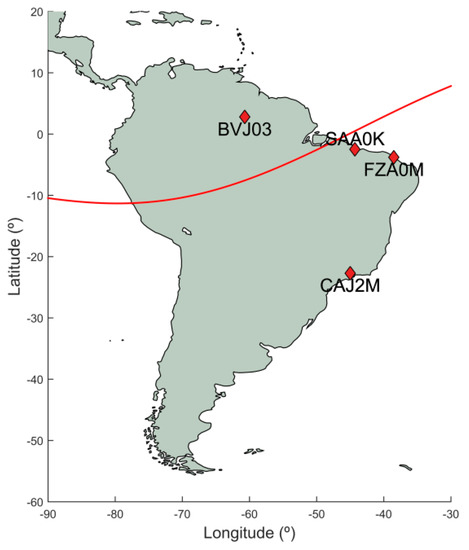
Figure 1.
Location of the four ionosondes used for the GIMs assessment.
The peculiarity of our validation method is that we form a pair of ionosonde stations. The foF2 variability of the ionosphere between both stations is considered as relatively close to the VTEC variability. To this end, Table 2 presents the selected pairs of ionosonde stations with their respective distances.
Table 2.
Six possible pair combinations of the four ionosondes and their respective distances.
We have applied the assessment method at different time series: one week; one year and four years. The first analysis aimed to select the assessment strategy with better performance, using one-week data from 2015 with the six possible ionosonde pair combinations (Table 2) and all the rapid and final GIMs (Table 1). In the second assessment, after the selection of the best strategy, we extended the application of this method for a one-year time series (2015), assessing all GIMs previously used. The third assessment was conducted with two of the products with the best performance in the 2015 time series, CODG and UQRG, considering a four-year time series (2014-2017).
The method of assessment proposed in this paper is based on the correlation between the critical frequency at the F2 layer and the VTEC [19,20,21]. Figure 2 presents plots comparing the behavior of foF2 measured by two pairs of ionosondes and the respective VTEC values estimated using two GIM products (CODG and UQRG) for the ionosonde positions. Values presented correspond to the day of year (DOY) 21 of 2015. It can be noticed that foF2 and VTEC in general present a clear similarity. Some specific behaviors of foF2 are not always well represented by VTEC but we assume that the quality depends on the GIM product.
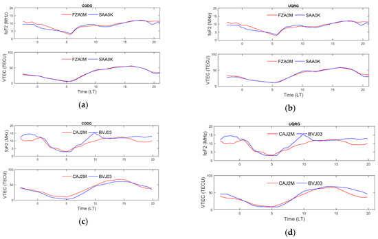
Figure 2.
Comparison of the foF2 measured with ionosondes and VTEC values estimated for the respective ionosondes using CODG (a,c) and UQRG (b,d).
In the proposed GIM assessment method, data from one ionosonde () is estimated based on data from the other ionosonde of the considered pair (). The VTEC variation between both places is used to transport the foF2 from ionosonde 2 to the location of the ionosonde 1. In this way, estimated foF2 can be compared with the real foF2 measured at the first ionosonde (), and, implicitly, the GIM quality can be assessed in front of a manually scaled foF2 measurement.
The GIM assessment was based on the root mean square (RMS) of the differences between the values of foF2 measured at the first station () and the values estimated with GIMs ():
where is the number of values estimated.
The assessment also considered the normalized root mean square (NRMS):
to confirm the results obtained.
The rates of improvement (RoI) were also calculated:
where represents the critical frequencies at the F2 layer measured at the second ionosonde.
Two equations were analyzed to carry out foF2 transportation. The first approach is based on the simple ratio between critical frequency and VTEC values, i.e., on the assumption of a direct linear correlation:
where and represent the vertical total electron content values interpolated for the ionosondes positions using a GIM product.
The second approach is based on the ratio of the squared critical frequency and VTEC values. Considering the relationship between frequency and VTEC in the ionospheric delay estimation:
we are implicitly assuming a linear correlation between VTEC and the peak density, NmF2. When taking into account the first-principles relationship between NmF2 and foF2 (see for instance Kelley [29]), we formulate the second approach as:
In addition to the approaches presented, we also evaluated the use of local time (LT) for the time-collocation vs. the usage of plain Universal Time (UT). In this way, we had analyzed four approaches, considering equation (4) with LT and UT and equation (6) using LT and UT for time-collocation.
In the method proposed, we consider that the behavior of foF2 is correlated to VTEC, assuming constant slab thickness. One limitation of this assumption is related to regions with significantly distinct ionosphere (and consequently different slab thickness in the two regions considered) [19,20,21]. To analyze this influence, in the first assessment section, we also estimated other ionospheric indicators. First, we analyzed the slab thickness () values [30]:
with representing the maximum electron density at the F2 layer, and, second, we have analyzed the inverse value of the slab thickness, or the shape function peak ():
which presents a higher spatial correlation than the electron density profiles [31].
3. Results
We present the main results divided into three sections. The first one concerns the selection of the best strategy to transport foF2 based on VTEC values. The second section presents further analysis with daily and weekly data, considering error versus time and distance and additional discussion concerning the estimation of two ionospheric indicators (slab thickness and shape function peak). In the third section, we present two time series analyses, the first with one-year data (2015) and thirteen GIMs and the last one with four-year data (2014–2017) and two ionospheric products.
3.1. Strategy Selection
To characterize the state of the ionosphere in the week used for the selection of the best strategy, Figure 3 presents two indices: Dst (Disturbance storm time), on the left, and F10.7 (solar radio flux at 10.7 cm), on the right. The period corresponds to days 20 to 26 of 2015, the indices were obtained at OMNIWEB [32]. It can be verified that no significant magnetic storms occurred in this week, the minimum Dst obtained (−34 nT) occurred on day 26, it was also the only value to reach the scale of a weak storm (−30 nT to −50 nT) [33]. Regarding the F10.7, the values are above 110, indicating the active influence of the Sun.
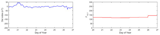
Figure 3.
Dst and F10.7 indices for the period of 020 to 026 of 2015.
Figure 4 presents the RMS of the differences between foF2 values estimated and measured during one week (DOYs 20 to 26 of 2015), involving an average number of 980 measurements per ionosonde. Each plot corresponds to the results of a distinct strategy, being the first strategy related to the Equation (4), named here as freq1, with UT time-colocation. The second strategy is related to freq1 using LT time-colocation. The third strategy is related to the squared frequency (freq2) of Equation (6) in UT; and the last is related to the squared frequency (freq2) in LT. The left panels show the ionosonde pair with the smallest distance and the right ones are referred to the pairs with the longest distance.
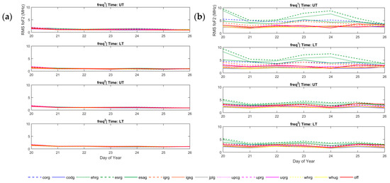
Figure 4.
One-week RMS values of the differences between foF2 values estimated with the help of the different GIMs to describe the foF2 variation between the values measured at the pair of ionosondes, considering the four approaches described for two pairs of ionosondes: (a) FZA0M and SAA0K, the smallest distance; and (b) CAJ2M and BVJ03, the longest distance.
Visually, the influence of the distance between the ionosondes and the error obtained is clear. The results on the right (longest distance) present larger differences and higher variability. It is also possible to notice that the approach considering the ratio with squared frequency of Equation (6) presents better performance for both pairs. Regarding the use of UT or LT, the selection of the best strategy is not so clear from Figure 4 only, except for the larger distance with the frequency ratio, where the use of LT provided better results.
Despite of presenting detailed results for two pairs, the other four ionosonde pairs also presented similar behavior. To summarize the values obtained and to allow the selection of the best strategy, we present in Table 3 the mean RMS errors obtained with the same dataset for the six ionosondes pairs. The values from the four approaches were classified from the smaller (lightest gray) to the largest (darkest gray) differences for each pair independently for each GIM. For instance, analyzing the first column of Table 3, i.e., the first pair (FZA0M and SAA0K) of CORG GIM, 0.87 (lightest gray) is the smallest value and 1.17 (darkest gray) is the largest value. In each row, the smaller values between the thirteen GIMs are highlighted in italic, indicating the product with better performance.
Table 3.
Mean RMS (MHz) of the differences between foF2 values measured and estimated with the four approaches presented, considering GIMs products and the simple difference between the values of both ionosondes (off). The error was computed for the week of 020 to 026 of 2015.
From this analysis, it can be noticed that the fourth strategy provided the lowest RMS values, which means that the strategy selected to assess GIMs was the ratio considering the squared frequency (Equation (6)) in LT collocation. Indeed, the influence of time transformation on LT is more significant with the simple ratio strategy than when the squared frequency is used in agreement with the typical stationarity of the electron content distribution on a sun-fixed reference frame motivated by the main solar ionization source. It can also be noticed that the larger differences in the time correction to LT are related to larger distances in longitude, once the correction is based on the longitude of the stations. For instance, for the ionosondes CAJ2M and SAA0K, which present similar longitudes (45.0W and 44.3W), the time correction is the same, as are the results in UT and LT, consequently. The results also showed that CODG and UQRG presented the best performance between the products analyzed for the week selected.
3.2. Daily and Weekly Analysis
Figure 5 presents the corresponding VTEC values and the estimated foF2 values at the locations of two pairs of ionosondes. Results presented correspond to the day of year (DOY) 21 of 2015. Again (a) and (b) are plots of the pair with a smaller distance and (c) and (d) are related to the pair with a larger distance. The green line indicates the foF2 values estimated to the location of the ionosondes represented by the red line, based on foF2 measurements from the ionosonde represented by blue lines. The left panels show the CODG GIMs solutions and the right panels show the UQRG solutions. The influence of the distance between the ionosondes is observed in both foF2 and VTEC values. The influence of VTEC can be noticed, for instance, around 10 h LT for the second pair (CAJ2M and BVJ03), where the foF2 measured at BVJ03 is larger than that at CAJ2M. In this case, UQRG better represented the ionospheric variability, leading to a closer estimation of foF2 to the values measured by the ionosonde.
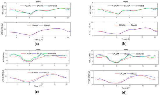
Figure 5.
Comparison of foF2 measured with ionosondes and the values estimated with GIMs versus VTEC values for the respective ionosondes using CODG (a,c) and UQRG (b,d).
Figure 6 presents the differences between the estimated and measured foF2 for one day of the same two pairs considered before (with the smallest (a) and largest (b) distances). For these same data, we also present the difference in slab thickness (Figure 7) and the shape function peak (Figure 8). The results obtained in the estimation of foF2 are correlated to the behavior of the ionosphere reflected by slab thickness and shape function peak. The shape function peak demonstrated to be a good indicator to characterize the ionospheric similarity between two regions. Values presented in Figure 8a are much more similar than those from the most distant pair (Figure 8b). Considering the values for the first pair, the highest variability of the RMS (Figure 6a) occurs close to 0 h, 05 h, and 20 h LT, when similar periods with larger differences were observed in the shape function peak estimation. The higher differences between FAZ0M and SAA0K are associated with the geomagnetic locations and the effects of the equatorial ionization anomaly (EIA). SAA0K is located closer to the magnetic equator, which leads to lower ionization in comparison to FAZ0M (closer to the EIA crest). The peak of difference after 18 LT in Figure 6a is associated with the post-sunset enhancement of ionization, where EIA becomes more evident due to the transition between nighttime and daytime [12]. In the case of CAJ2M and BVJ03 (Figure 6b), they are located at a distinct magnetic hemisphere, with a large distance apart from them, and several reasons justify large foF2 differences, such as the EIA asymmetries, recombination rates, solar zenith angle, geomagnetic field configurations, and seasonal variabilities.
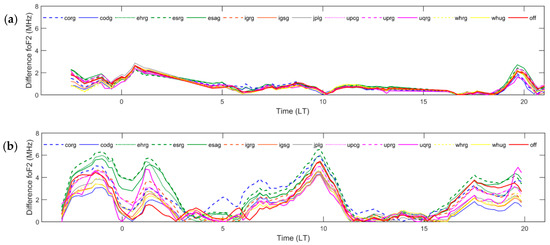
Figure 6.
Differences between foF2 values measured at the ionosondes and estimated using GIMs, for two pairs of ionosondes: (a) FZA0M and SAA0K, the closest one; (b) CAJ2M and BVJ03, the most distant one.
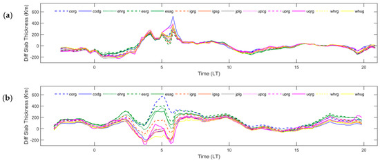
Figure 7.
Differences between slab thickness are estimated for the ionosonde positions of two pairs of ionosondes: (a) FZA0M and SAA0K, the closest one; and (b) CAJ2M and BVJ03, the most distant one.
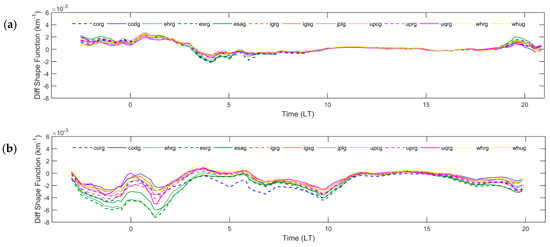
Figure 8.
Differences between shape function peak estimated for the ionosonde positions of two pairs of ionosondes: (a) FZA0M and SAA0K, the closest one; (b) CAJ2M and BVJ03, the most distant one.
Figure 9a shows the mean RMS differences of estimated foF2 and measured for one-week data versus the distance of the ionosondes. This indicates that most of the GIM products provide better results predicting the foF2 spatial variability than directly comparing data from both ionosondes (red line), even when great distances are considered. To verify the influence of ionospheric electron content on error behavior, we present the results from two more weeks in Figure 9: (b) days 166-172 of 2015, period with lower electron content; and (c) days 288-294 of 2015, period with larger electron content. The results indicate that in periods of lower ionospheric electron content, the use of any GIM provides better results than the direct comparison of data from both ionosondes, and the worst performance of some of the products occurred in periods of high ionospheric electron content. However, in general, the performance of the approach with GIMs was better, for most of the products available, than not using any GIM.
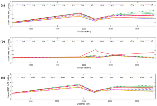
Figure 9.
Mean RMS of the differences between foF2 values measured at the ionosondes and estimated using GIMs versus the distance of the ionosondes pairs considering one-week data: (a) test week (020-026/2015); (b) low (166-172/2015); (c) high (288-294/2015) ionospheric electron content.
Figure 9 clearly shows that the increase of the error is not only affected by the distance, but also by other factors, such as the region of the ionosondes considered. Figure 10 presents the same results now divided into two sections: one with the pairs formed with CAJ2M ionosonde (right), located at different latitudes, and one with the other three pairs (left). It can be noticed that the influence of distance has a different impact on the two sections. In the section of pairs at similar latitude (left), the increase of the error related to the distance happens in the period with low electron content (b), for the other section the relation is valid for the period with high electron content (c). Considering the pairs without CAJ2M, the decrease occurs with the pair of ionosondes FZA0M and BVJ03, this behavior could be related to the location of the stations. SAA0K is located closer to the magnetic equator than the other two ionosondes, so in the period with high electron content, the proximity with the equator could lead to a more significant difference in the ionospheric influence, compared to the other station. Considering the pairs with CAJ2M, as previously mentioned, several sources of influence are involved, such as EIA asymmetries, seasonal variabilities, and recombination rates. In addition, this figure also shows the significant improvement in the results with the use of GIMs for the period with lower electron content considering pairs with CAJ2M (b).
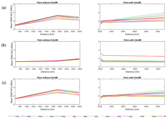
Figure 10.
Mean RMS of the differences between foF2 values measured at the ionosondes and estimated using GIMs versus the distance of the ionosondes pairs considering one-week data divided into pairs formed with ionosondes at different (right) and similar (left) latitudes: (a) test week (020-026/2015); (b) low (166-172/2015); (c) high (288-294/2015) ionospheric electron content.
3.3. Time Series Analysis
Figure 11 presents Dst (left) and F10.7 (right) indices for the years 2014 (a), 2015 (b), 2016 (c), and 2017 (d). Dst indices indicate the occurrence of some storms, including strong ones in the four years (−100 nT to −200 nT) and two severe storms in 2015 (−200 nT to −350 nT) [33]. F10.7 indicates active sun, in addition, it can be noticed the decrease of the solar activity from 2014 (solar cycle peak) to 2017.
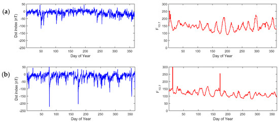
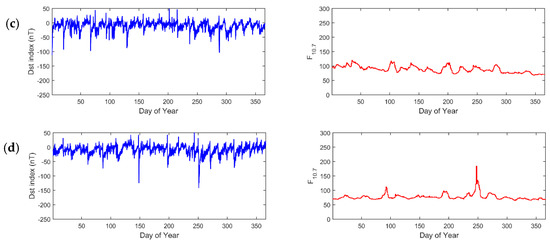
Figure 11.
Dst and F10.7 indices for the period of 1 to 365 of 2014 (a), 2015 (b), 2016 (c) and 2017 (d).
Figure 12 shows the RMS of foF2 differences for 2015 considering the thirteen GIMs and the six ionosonde pairs. Considering the general results, the seasonal influence can be noticed for all the pairs, with higher values from October to March, a period with higher ionospheric electron content in the Southern Hemisphere. In addition, the three pairs with ionosonde CAJ2M presented a higher improvement with the use of GIMs from March to October. It is worth highlighting that CAJ2M is the ionosonde with larger distances in latitude compared to the others, so the behavior of the ionosphere is less similar in this region. The results indicated that for the period with less intense ionospheric electron content, the use of GIMs led to significant improvement in the representation of the different regions considered, confirming the behavior observed in Figure 10b. That indicates this scenario like the one where the use of the GIMs presented the strongest improvements. On the other hand, when a period with higher ionospheric electron content is considered, the error estimated with the help of the GIMs is closer to the simple difference between the values of the ionosondes. These results indicate that besides being a challenging region, when periods with lower ionospheric electron content are considered, GIMs can be able to represent the Brazilian ionospheric variability. However, when periods with higher electron content are considered, the performance of GIMs representing the ionosphere in this region may not be so realistic. The worse performance of GIMs in this period can also be related to the increase of the ionospheric gradients that affect foF2 (local measurement) in a different way than VTEC (integrated measurements). The different influence in the foF2 and VTEC can be provided by the slab thickness, that in the case of the presented method is assumed to be constant. In this way, a worse performance of the method was expected, when regions and periods with different ionospheric gradients are considered. More details on the influence of slab thickness in the relations between foF2 and VTEC can be found in Spalla and Ciraolo [19], Leitinger et al. [20], and Kouris et al. [21]. Regarding the general performance of GIMs, it is worth mentioning the consistency of most of the products, presenting similar behavior, mainly if only the final products are considered, similar to other GIM assessment techniques [2].
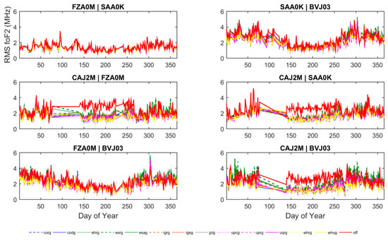
Figure 12.
RMS values of the differences between foF2 values estimated with GIMs and measured at the ionosondes for the six pairs of ionosondes for one-year data (2015).
Table 4 summarizes the mean RMS of the values from 2015 for each product. Table 5 presents the mean improvement percentages compared with the simple difference of the ionosondes foF2, without the representation of the ionospheric variation from GIM. Products with the best improvement rates are highlighted in gray. The lowest rates of improvements were observed in the pair with the smaller distance between the ionosondes, and the highest in the pair with a higher distance. This indicates the relevance of representing the ionospheric variability, especially when larger distances are considered. Analysis using NRMS values presented similar behavior to that obtained with RMS values, confirming the RMS analyses.
Table 4.
One-year (2015) mean RMS values of the differences between foF2 values measured and estimated with GIMs and the simple difference between the values of both ionosondes (off).
Table 5.
Rates of improvement considering one-year (2015) mean RMS values of the differences between foF2 values measured and estimated with GIMs.
In Figure 13, we present the mean RMS from 2015 for each product versus distance. The results show an expected increase in the mean error related to the distance of the ionosonde and that even the products with a worse performance presented improvements in the estimation of critical frequency, compared with the approach without GIM information. These results confirm what was previously indicated with one-week data, and show that, on average, the results with GIM data presented a better performance than the simple differences between the measured values.
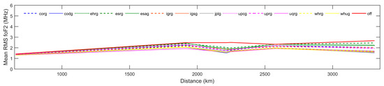
Figure 13.
Mean RMS of the differences between foF2 values measured at the ionosondes and estimated using GIMs versus the distance of the ionosondes pairs considering one-year data (2015).
The products with the highest rates of improvement were CODG, IGSG, JPLG, UQRG, WHRG, and WHUG (Table 5). From those products, we selected two (CODG and UQRG) to analyze the RMS of the differences in foF2 estimation considering four years (Figure 14): 2014 (a), 2015 (b), 2016 (c), and 2017 (d). The same behavior noticed with all the GIMs in 2015 can be observed for CODG and UQRG for the other considered years, except the one considering the ionosonde CAJ2M in 2014, due to lack of data. In addition, with the four-year time series, it is also possible to notice the influence of the solar cycle. The results show that higher RMS occurred closer to the last solar cycle peak (between 2013 and 2014).
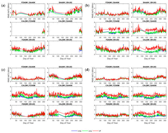
Figure 14.
RMS values of the differences between foF2 values estimated with two GIMs products (CODG and UQRG) and measured at the ionosondes for the six pairs of ionosondes for one-year data: (a) 2014; (b) 2015; (c) 2016; (d) 2017.
Table 6 summarizes the results presenting the mean RMS values, and Table 7 presents the percentages of improvement compared to the simple difference of the values measured at the ionosondes. In general, as noticed for 2015, the lowest rates of improvement were observed for the pair with the closest ionosondes, at similar latitudes and the highest rates for the most distant pair, involving ionosondes at quite different latitudes. As observed in the RMS values from Figure 13, the rates of improvement also do not follow a regular increase related to the distance. Considering the proximity of the solar cycle peak, it was not possible to notice a clear pattern of improvement for all the pairs. For instance, in the closest pair, the rate improvement decreases, and in the most distant pair, the rate tended to increase. In general, the pairs with ionosondes with a larger difference in latitude (CAJ2M_FZA0M, CAJ2M_SAA0K, and CAJ2M_BVJ03) tended to present an increase in the rates of improvement for data closer to solar minimum, while the pairs with ionosondes with closer latitudes (FZA0M_SAA0K, SAA0K_BVJ03, and FZA0M_BVJ03) tended to present a decrease in the rates of improvement. In fact, by Table 6, considering columns ‘off’ (indicating the simple difference between the foF2 of both ionosondes), gradients from each pair can be compared. This is consistent with the gradient for ionosondes in similar latitudes (spatio-longitudinal), which decrease from solar maximum (2014) to the solar minimum (2017); with the ionosondes in different latitudes (spatio-latitudinal) for which the gradient slightly varies (increase or decrease).
Table 6.
One-year mean RMS values of the differences between foF2 values measured and estimated with GIMs (CODG and UQRG) and the simple difference between the values of both ionosondes (off).
Table 7.
Rates of improvement considering one-year mean RMS values of the differences between foF2 values measured and estimated with two GIMs products (CODG and UQRG).
4. Discussion
We have presented a new way of assessing GIMs, by looking at how much they can help in the interpolation of directly measured and manually scaled foF2, applied up to four years of data in one of the most challenging ionospheric scenarios that we can have: low latitude and around the most recent solar maximum. The best strategy, linear interpolation of squared foF2 based on VTEC ratio, is in agreement with the good behavior of the shape function (electron density divided by the corresponding VTEC) for modeling radio occultations [31].
The performance of the different GIMs presented consistency, especially considering the final products. The highest errors and smaller rates of improvement were obtained with rapid products. The agreement of IGS GIMs was also observed in the assessment performed by Roma-Dollase et al. [2]. Concerning the performance over the Brazilian region, the main improvements were observed in the period of lower ionospheric electron content, considering pairs with ionosondes in different latitudes. This highlights the relevance of the use of GIMs information to approximate the variability of the ionosphere. It could also indicate some limitations of the ionospheric modeling in the Brazilian region in periods with larger electron content. That performance can also be related to the limitation of the method when periods and regions with different slab thickness values are considered. This in agreement with the behavior presented in Spalla and Ciraolo [19], Leitinger et al. [20], and Kouris et al. [21].
Many efforts have been made to model and monitor the ionosphere, especially due to its impact on activities as the ones related to GNSS. Many ionospheric assessment methods rely on ionosonde data, which can be tricky when a limited number of ionosondes are available, mainly considering regions with high ionospheric variability. In this way, the method presented may also be an alternative approach to assessing ionospheric models, by using ionosonde data aided by GIM. A limitation observed in the method is related to periods with significant differences in the ionospheric behavior of the considered regions. A possible improvement of the method could be the use of filtering based on an ionospheric indicator, such as the shape function peak estimation, to identify periods and regions when the method can be applied.
5. Conclusions
This paper presented a new method for assessing global ionospheric maps (GIM) by means of ionosonde data. Four strategies were presented, the best one was the linear interpolation of squared foF2 based on the VTEC ratio. The assessment was performed over one of the most challenging scenarios, the Brazilian region and near the last solar cycle peak. The analyses are considered daily, weekly, one-year, and four-year time series and thirteen of the main GIMs products available. The analysis was based on the RMS values and additional ionospheric indicators, slab thickness, and shape function peak were used to complement the daily analysis.
Regarding the application of the method in the Brazilian region, error increase related to distance and seasonal influence could be noticed, with larger errors near 2014 (solar cycle peak) and especially considering pairs with ionosondes in different latitudes. Considering the GIMs selected, CODG, IGSG, JPLG, UQRG, WHRG, and WHUG provided the best improvement in 2015, with mean rates of improvement between 5% and 42% in comparison to not using any GIM. With data from 2014-2017, CODG and UQRG provided improvement rates from 5% up to 49%.
Author Contributions
Conceptualization, G.O.J. and M.H.-P.; Formal analysis, G.O.J., M.H.-P., F.S.P., D.B.M.A. and J.F.G.M.; Methodology, G.O.J. and M.H.-P.; Supervision, M.H.-P.; Writing—original draft, G.O.J., M.H.-P., F.S.P., D.B.M.A. and J.F.G.M.; Writing—review & editing, G.O.J., M.H.-P., F.S.P., D.B.M.A. and J.F.G.M. All authors have read and agreed to the published version of the manuscript.
Funding
This study was financed in part by the Coordenação de Aperfeiçoamento de Pessoal de Nível Superior—Brasil (CAPES)—Finance Code 001 with the support as well of the UPC.
Acknowledgments
We acknowledge INPE for providing the ionosonde data, the IGS IAACs, in particular, CODE, ESA, JPL, UPC, and WHU, for providing global ionospheric maps and the National Institute of Science and Technology for GNSS in Support of Air Navigation (INCT GNSS-NavAer), funded by CNPq (465648/2014-2), FAPESP (2017/50115-0), and CAPES (88887.137186/2017-00).
Conflicts of Interest
The authors declare no conflict of interest. The funders had no role in the design of the study; in the collection, analyses, or interpretation of data; in the writing of the manuscript, or in the decision to publish the results.
References
- Hernández-Pajares, M.; Juan, J.; Sanz, J.; Orus, R.; Garcia-Rigo, A.; Feltens, J.; Komjathy, A.; Schaer, S.; Krankowski, A. The IGS VTEC maps: A reliable source of ionospheric information since 1998. J. Geod. 2009, 83, 263–275. [Google Scholar] [CrossRef]
- Roma-Dollase, D.; Hernández-Pajares, M.; Krankowski, A.; Kotulak, K.; Ghoddousi-Fard, R.; Yuan, Y.; Li, Z.; Zhang, H.; Shi, C.; Wang, C.; et al. Consistency of seven different GNSS global ionospheric mapping techniques during one solar cycle. J. Geod. 2017, 92, 691–706. [Google Scholar] [CrossRef]
- Bilitza, D.; Altadill, D.; Truhlik, V.; Shubin, V.; Galkin, I.; Reinisch, B.; Huang, X. International Reference Ionosphere 2016: From ionospheric climate to real-time weather predictions. Space Weather 2017, 15, 418–429. [Google Scholar] [CrossRef]
- Kilifarska, N.A.; Ouzounov, D.P. Theoretical modeling of foF2 and hmF2 ionospheric parameters during a strong magnetic disturbance. J. Geophys. Res. Space Phys. 2001, 106, 30415–30428. [Google Scholar] [CrossRef]
- Odeyemi, O.O.; Adeniyi, J.O.; Oladipo, O.A.; Olawepo, A.O.; Adimula, I.A.; Oyeyemi, E.O. Investigation on slab-thickness and B0 over an equatorial station in Africa and comparison with IRI model. J. Atmos. Sol. Terr. Phys. 2018, 179, 293–306. [Google Scholar] [CrossRef]
- Hu, A.; Carter, B.; Currie, J.; Norman, R.; Wu, S.; Wang, X.; Zhang, K. Modeling of topside ionospheric vertical scale height based on ionospheric radio occultation measurements. J. Geophys. Res. Space Phys. 2019, 124, 4926–4942. [Google Scholar] [CrossRef]
- Liu, A.; Wang, N.; Li, Z.; Wang, Z.; Yuan, H. Assessment of NeQuick and IRI-2016 models during different geomagnetic activities in global scale: Comparison with GPS-TEC, dSTEC, Jason-TEC and GIM. Adv. Space Res. 2019, 63, 3978–3992. [Google Scholar] [CrossRef]
- Wang, N.; Li, Z.; Yuan, Y.; Li, M.; Huo, X.; Yuan, C. Ionospheric correction using GPS Klobuchar coefficients with an empirical night-time delay model. Adv. Space Res. 2019, 63, 886–896. [Google Scholar] [CrossRef]
- Goss, A.; Schmidt, M.; Erdogan, E.; Seitz, F. Global and Regional High-Resolution VTEC Modelling Using a Two-Step B-Spline Approach. Remote Sens. 2020, 12, 1198. [Google Scholar] [CrossRef]
- Garcia-Fernandez, M.; Hernandez-Pajares, M.; Juan, J.M.; Sanz, J. Performance of the improved Abel transform to estimate electron density profiles from GPS occultation data. GPS Solut. 2005, 9, 105–110. [Google Scholar] [CrossRef]
- Habarulema, J.B.; Ssessanga, N. Adapting a climatology model to improve estimation of ionosphere parameters and subsequent validation with radio occultation and ionosonde data. Space Weather 2016, 15, 84–98. [Google Scholar] [CrossRef]
- Prol, F.; Camargo, P.; Hernández-Pajares, M.; Muella, M. A new method for ionospheric tomography and its assessment by ionosonde electron density, GPS TEC, and single-frequency PPP. IEEE Trans. Geosci. Remote Sens. 2018, 57, 2571–2582. [Google Scholar] [CrossRef]
- Ho, C.M.; Wilson, B.D.; Mannucci, A.J.; Lindqwister, U.J.; Yuan, D.N. A comparative study of ionospheric total electron content measurements using global ionospheric maps of GPS, TOPEX radar, and the Bent model. Radio Sci. 1997, 32, 1499–1512. [Google Scholar] [CrossRef]
- Hernández-Pajares, M.; Roma-Dollase, D.; Krankowski, A.; García-Rigo, A.; Orús-Pérez, R. Methodology and consistency of slant and vertical assessments for ionospheric electron content models. J. Geod. 2017, 91, 1405–1414. [Google Scholar] [CrossRef]
- Erdogan, E.; Schmidt, M.; Goss, A.; Görres, B.; Seitz, F. Adaptive Modeling of the Global Ionosphere Vertical Total Electron Content. Remote Sens. 2020, 12, 1822. [Google Scholar] [CrossRef]
- Araujo-Pradere, E.; Weatherhead, E.; Dandenault, P.; Bilitza, D.; Wilkinson, P.; Coker, C.; Akmaev, R.; Beig, G.; Buresová, D.; Paxton, L.; et al. Critical issues in ionospheric data quality and implications for scientific studies. Radio Sci. 2019, 54, 440–454. [Google Scholar] [CrossRef]
- Altinay, O.; Tulunay, E.; Tulunay, Y. Forecasting of ionospheric critical frequency using neural networks. Geophys. Res. Lett. 1997, 24, 1467–1470. [Google Scholar] [CrossRef]
- Pietrella, M.; Perrone, L. A local ionospheric model for forecasting the critical frequency of the F2 layer during disturbed geomagnetic and ionospheric conditions. Ann. Geophys. 2008, 26, 323–334. [Google Scholar] [CrossRef][Green Version]
- Spalla, P.; Ciraolo, L. TEC and foF2 comparison. Ann. Geophys. 1994, 37, 929–938. [Google Scholar] [CrossRef]
- Leitinger, R.; Ciraolo, L.; Kersley, L.; Kouris, S.S.; Spalla, P. Relations between electron content and peak density: Regular and extreme behaviour. Ann. Geophys. 2004, 47, 1093–1107. [Google Scholar] [CrossRef]
- Kouris, S.S.; Xenos, T.D.; Polimeris, K.V.; Stergiou, D. TEC and foF2 variations: Preliminary results. Ann. Geophys. 2004, 47. [Google Scholar] [CrossRef]
- Cander, L.R. Spatial correlation of foF2 and vTEC under quiet and disturbed ionospheric conditions: A case study. Acta Geophys. 2007, 55, 410–423. [Google Scholar] [CrossRef]
- Gerzen, T.; Jakowski, N.; Wilken, V.; Hoque, M. Reconstruction of F2 layer peak electron density based on operational vertical total electron content maps. Ann. Geophys. 2013, 31, 1241–1249. [Google Scholar] [CrossRef][Green Version]
- Krankowski, A.; Shagimuratov, I.I.; Baran, L.W. Mapping of foF2 over Europe based on GPS-derived TEC data. Adv. Space Res. 2007, 39, 651–660. [Google Scholar] [CrossRef]
- Ssessanga, N.; Mckinnell, L.A.; Habarulema, J.B. Estimation of foF2 from GPS TEC over the South African region. J. Atmos. Sol. Terr. Phys. 2014, 112, 20–30. [Google Scholar] [CrossRef]
- Pignalberi, A.; Habarulema, J.B.; Pezzopane, M.; Rizzi, R. On the development of a method for updating an empirical climatological ionospheric model by means of assimilated vTEC measurements from a GNSS receiver network. Space Weather 2019, 17, 1131–1164. [Google Scholar] [CrossRef]
- CDDIS. Available online: https://cddis.nasa.gov/Data_and_Derived_Products/GNSS/atmospheric_products.html (accessed on 16 May 2020).
- EMBRACE. Available online: http://www2.inpe.br/climaespacial/SpaceWeatherDataShare/search/ (accessed on 21 May 2020).
- Kelley, M.C. The Earth’s Ionosphere: Plasma Physics and Electrodynamics; Academic Press: Cambridge, MA, USA, 2009. [Google Scholar]
- Titheridge, J. The slab thickness of the mid-latitude ionosphere. Planet. Space Sci. 1973, 21, 1775–1793. [Google Scholar] [CrossRef]
- Hernández-Pajares, M.; Juan, J.; Sanz, J. Improving the Abel inversion by adding ground GPS data to LEO radio occultations in ionospheric sounding. Geophys. Res. Lett. 2000, 27, 2473–2476. [Google Scholar] [CrossRef]
- OMNIWEB. Available online: https://omniweb.gsfc.nasa.gov/form/dx1.html (accessed on 14 October 2020).
- Loewe, C.A.; Prölss, G.W. Classification and mean behavior of magnetic storms. J. Geophys. Res. Space Phys. 1997, 102, 14209–14213. [Google Scholar] [CrossRef]


Publisher’s Note: MDPI stays neutral with regard to jurisdictional claims in published maps and institutional affiliations. |
© 2020 by the authors. Licensee MDPI, Basel, Switzerland. This article is an open access article distributed under the terms and conditions of the Creative Commons Attribution (CC BY) license (http://creativecommons.org/licenses/by/4.0/).