Mapping Soil Organic Carbon for Airborne and Simulated EnMAP Imagery Using the LUCAS Soil Database and a Local PLSR

 ,
,  ,
,  and
and
Abstract

1. Introduction
2. Materials and Methods
2.1. Data
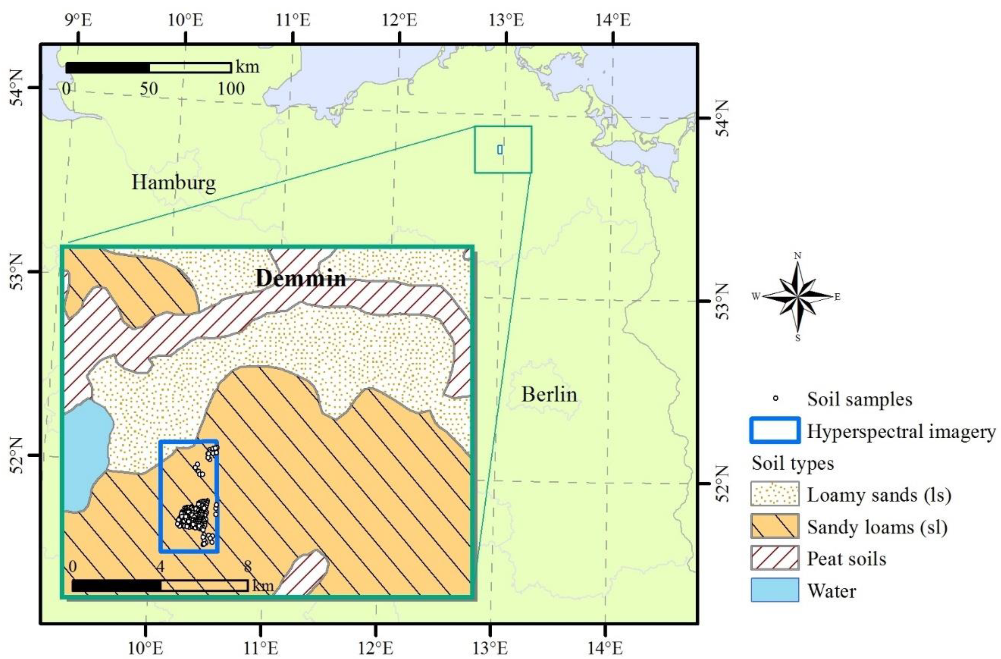
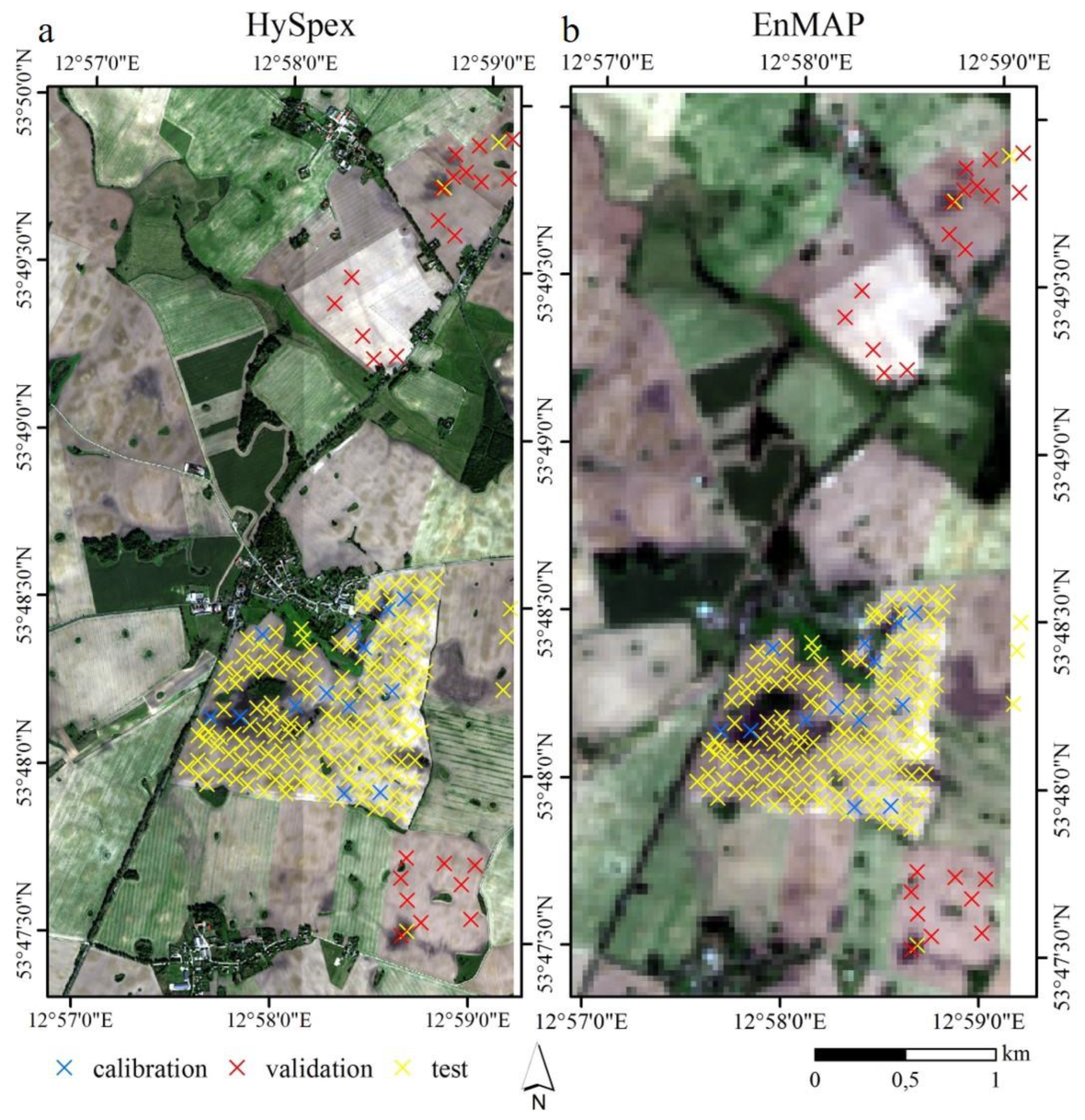
2.1.1. Study Site
2.1.2. LUCAS Soil Database
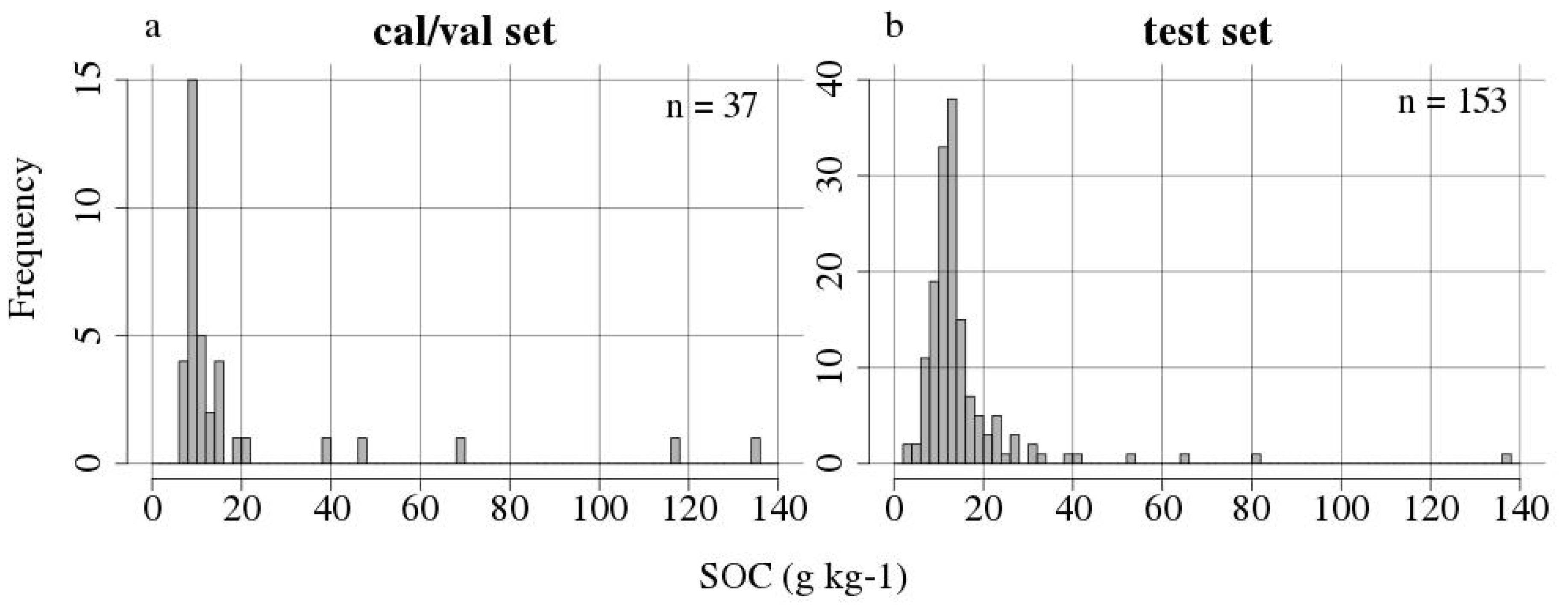
2.1.3. Field Soil Samples
2.1.4. Remote Sensing Imagery
2.2. Methods
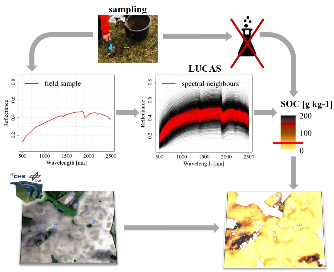
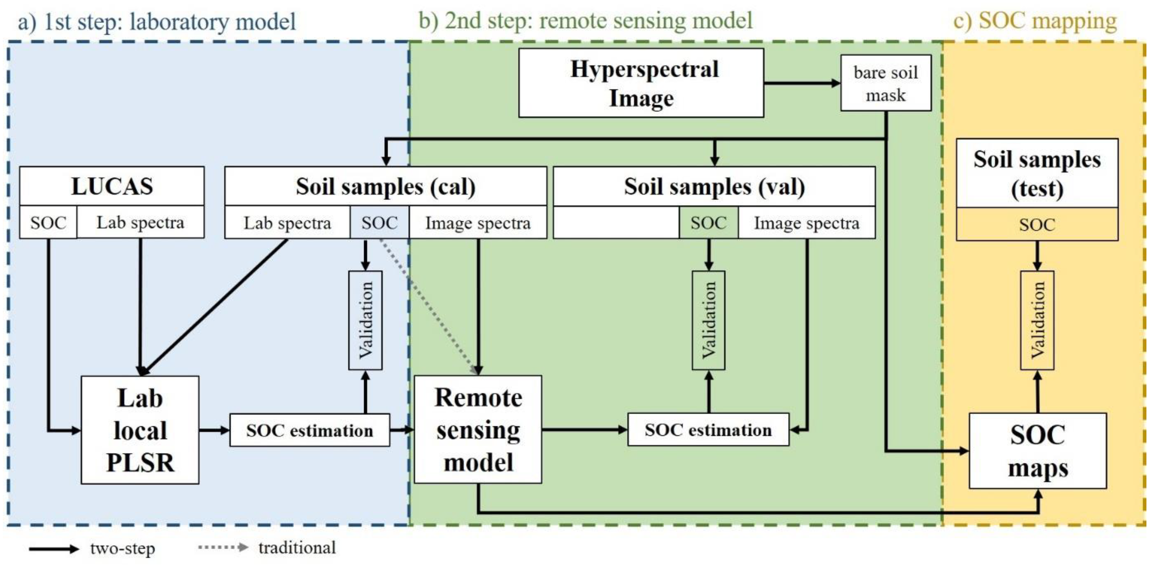
2.2.1. Overview and Concept
2.2.2. Data Pre-Processing
2.2.3. First Step: Laboratory SOC Modelling
2.2.4. Second Step: Remote Sensing SOC Modelling
3. Results
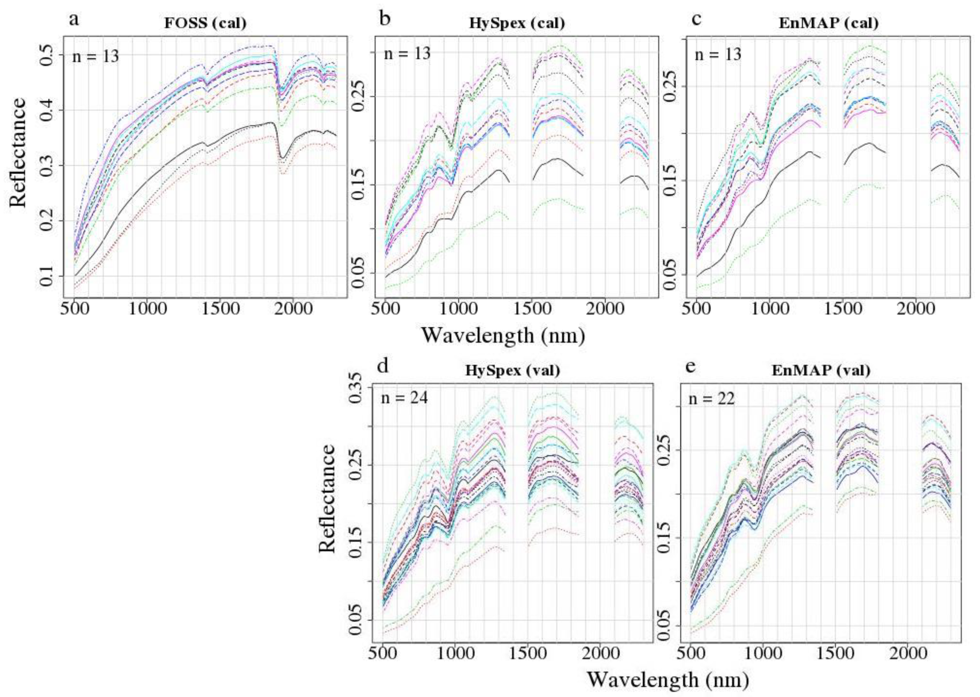
3.1. Spectral Data
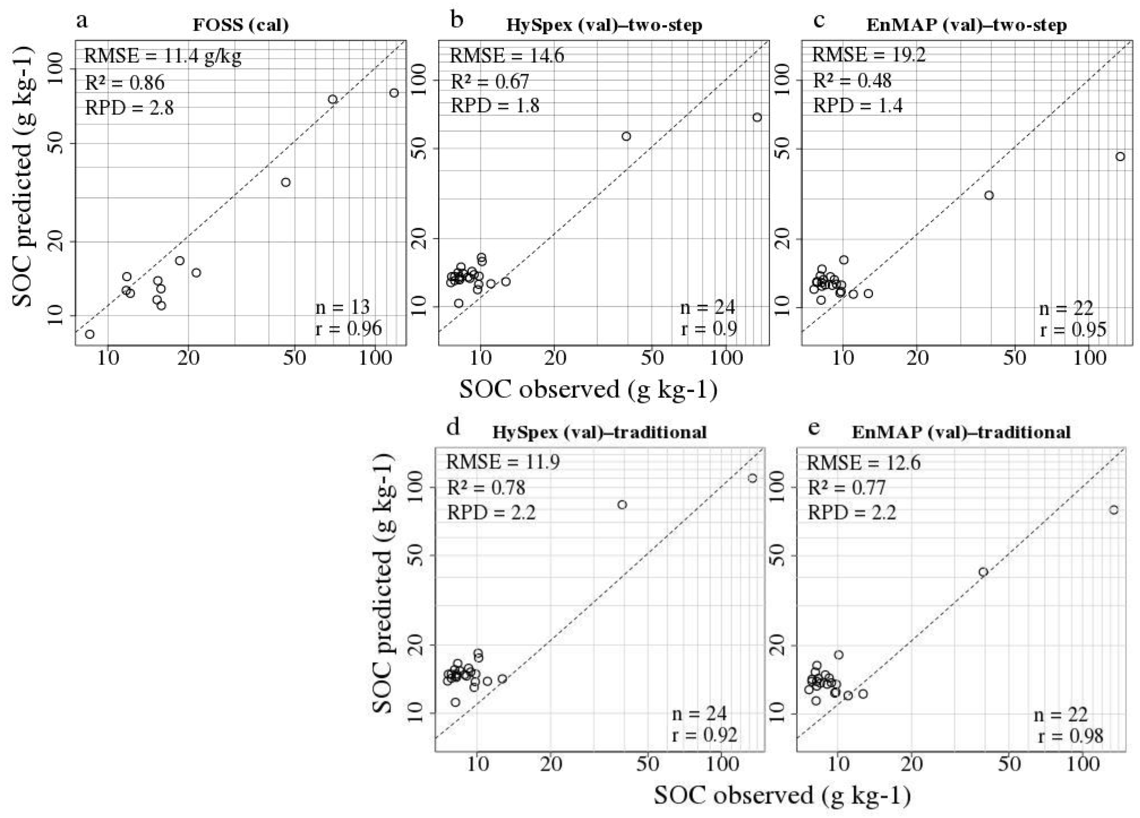
3.2. Laboratory SOC Modelling
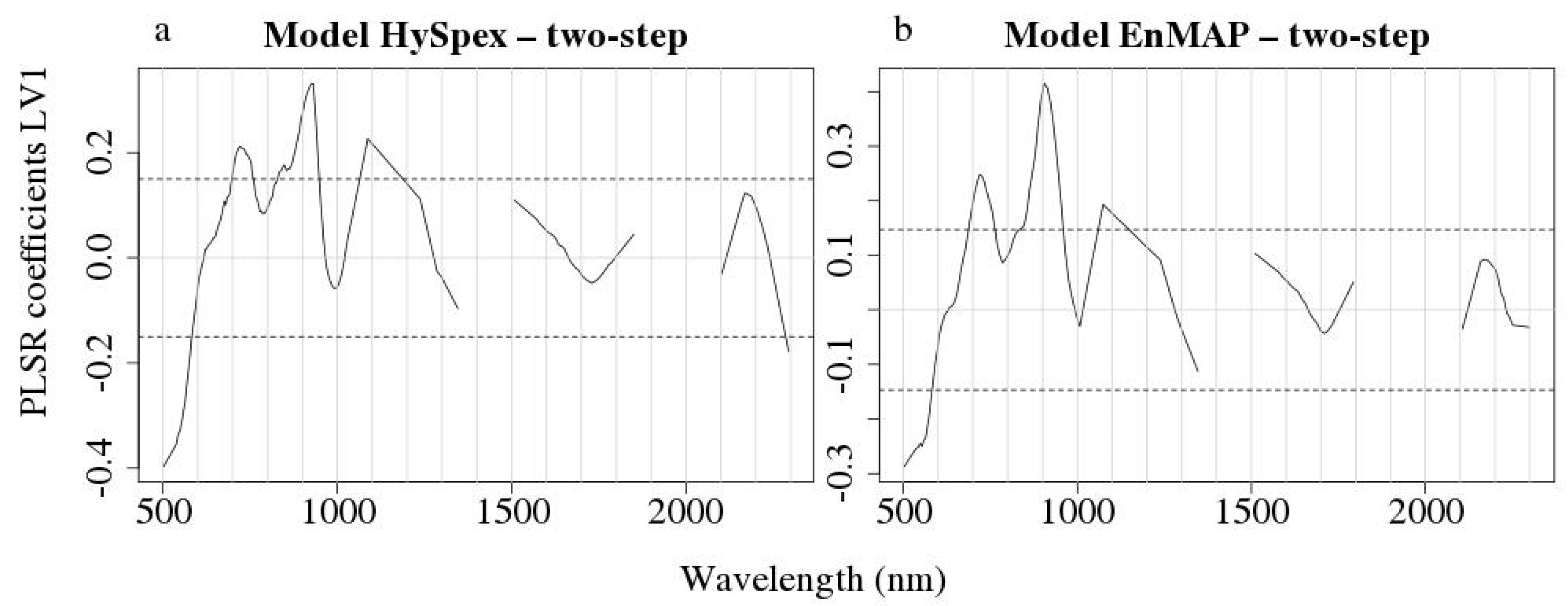
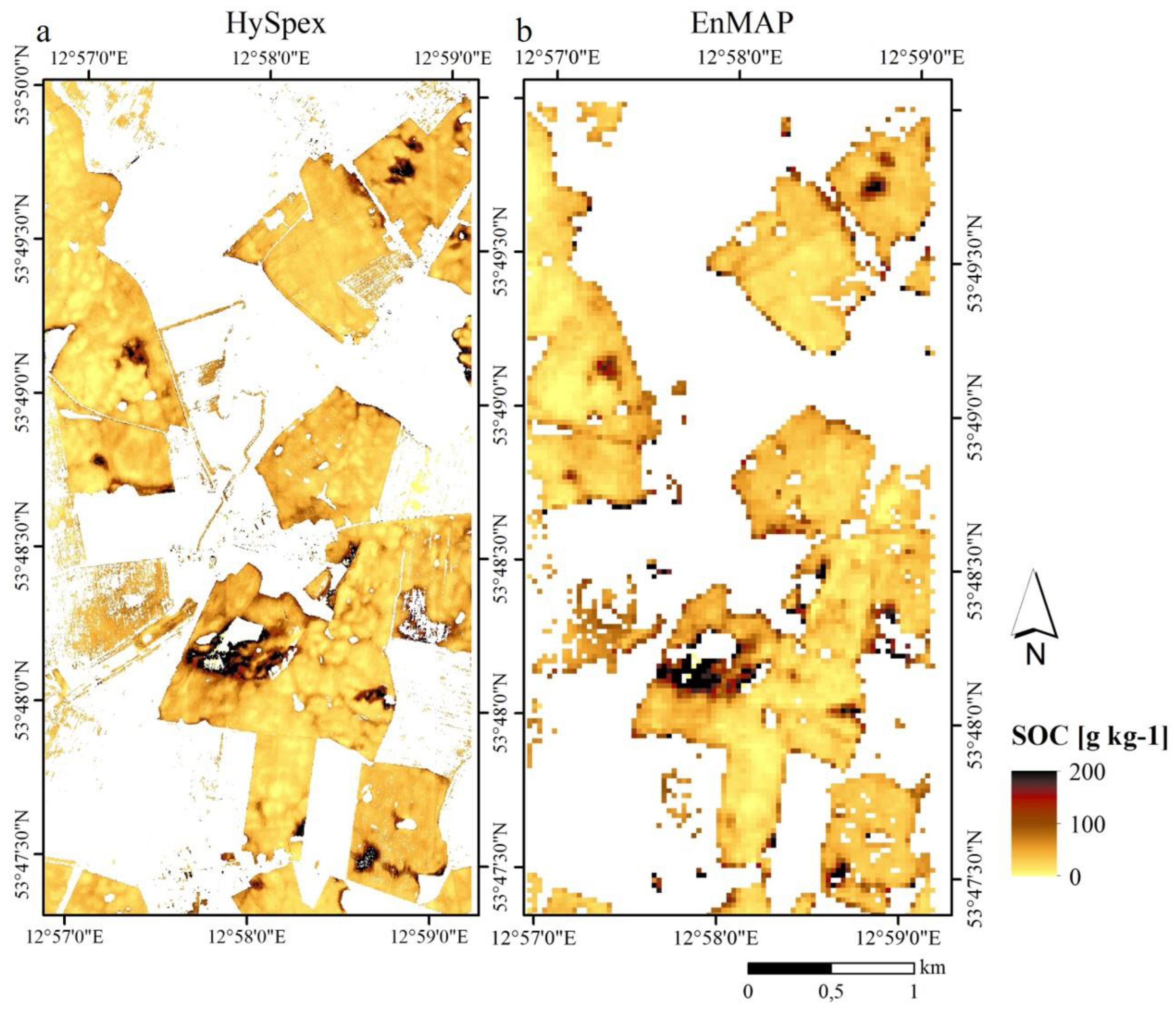
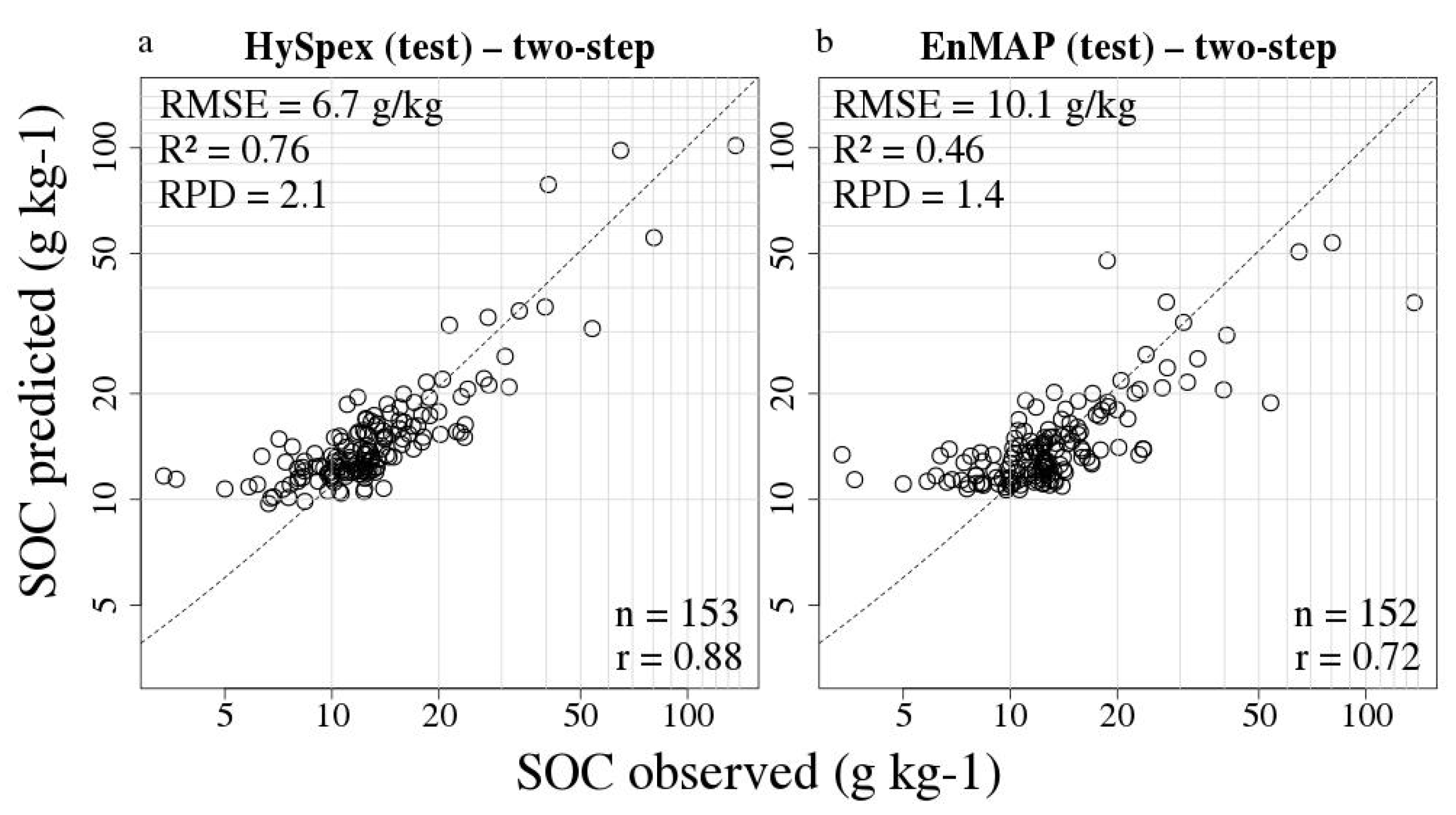
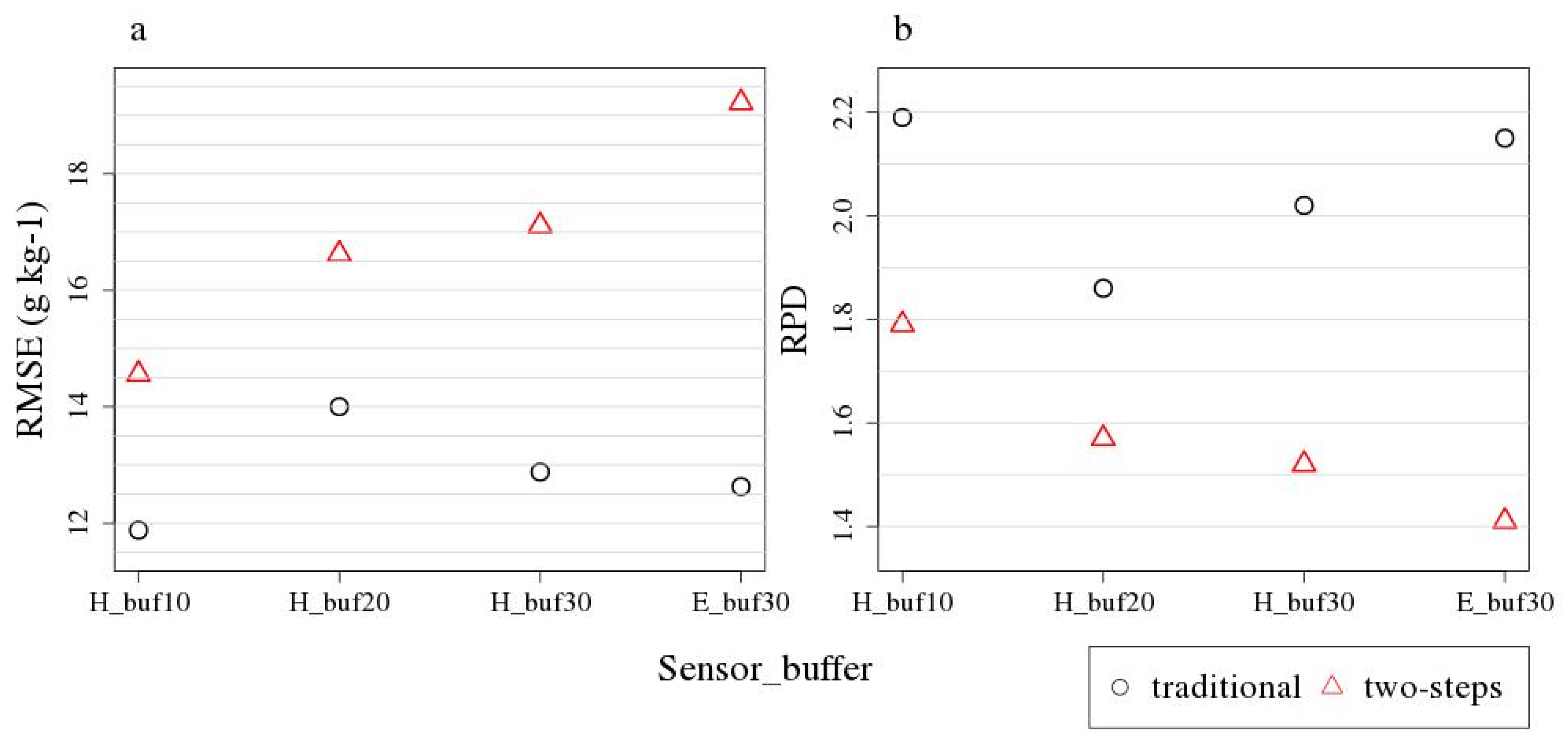
3.3. Remote Sensing SOC Modelling
4. Discussion
5. Conclusions
Author Contributions
Funding
Acknowledgments
Conflicts of Interest
References
- Lal, R. Soil carbon sequestration impacts on global climate change and food security. Science 2004, 304, 1623–1627. [Google Scholar] [CrossRef] [PubMed]
- Tóth, G.; Hermann, T.; da Silva, M.R.; Montanarella, L. Monitoring soil for sustainable development and land degradation neutrality. Environ. Monit. Assess. 2018, 190, 57. [Google Scholar] [CrossRef]
- Wiesmeier, M.; Urbanski, L.; Hobley, E.; Lang, B.; von Lützow, M.; Marin-Spiotta, E.; van Wesemael, B.; Rabot, E.; Ließ, M.; Garcia-Franco, N. Soil organic carbon storage as a key function of soils-a review of drivers and indicators at various scales. Geoderma 2019, 333, 149–162. [Google Scholar] [CrossRef]
- World Meteorological Organization (WMO). The Global Observing System for Climate: Implementation Needs. WMO Pub No. GCOS—200. 2016. Available online: https://public.Wmo.Int/en/programmes/global-climate-observing-system/ (accessed on 7 October 2020).
- Chabrillat, S.; Ben-Dor, E.; Cierniewski, J.; Gomez, C.; Schmid, T.; Van Wesemael, B. Imaging spectroscopy for soil mapping and monitoring. Surv. Geophys. 2019, 40, 361–399. [Google Scholar] [CrossRef]
- Conant, R.T.; Ogle, S.M.; Paul, E.A.; Paustian, K. Measuring and monitoring soil organic carbon stocks in agricultural lands for climate mitigation. Front. Ecol. Environ. 2011, 9, 169–173. [Google Scholar] [CrossRef]
- Kibblewhite, M.G.; Miko, L.; Montanarella, L. Legal frameworks for soil protection: Current development and technical information requirements. Curr. Opin. Environ. Sustain. 2012, 4, 573–577. [Google Scholar] [CrossRef]
- Nocita, M.; Stevens, A.; van Wesemael, B.; Aitkenhead, M.; Bachmann, M.; Barthes, B.; Ben Dor, E.; Brown, D.J.; Clairotte, M.; Csorba, A.; et al. Soil spectroscopy: An alternative to wet chemistry for soil monitoring. Adv. Agron. 2015, 132, 139–159. [Google Scholar]
- Beyer, L.; Kahle, P.; Kretschmer, H.; Wu, Q. Soil organic matter composition of man-impacted urban sites in north germany. J. Plant Nutr. Soil Sci. 2001, 164, 359–364. [Google Scholar] [CrossRef]
- Ben-Dor, E.; Inbar, Y.; Chen, Y. The reflectance spectra of organic matter in the visible near-infrared and short wave infrared region (400–2500 nm) during a controlled decomposition process. Remote Sens. Environ. 1997, 61, 1–15. [Google Scholar] [CrossRef]
- He, T.; Wang, J.; Lin, Z.; Cheng, Y. Spectral features of soil organic matter. Geo-Spat. Inf. Sci. 2009, 12, 33–40. [Google Scholar] [CrossRef]
- Viscarra Rossel, R.; Behrens, T. Using data mining to model and interpret soil diffuse reflectance spectra. Geoderma 2010, 158, 46–54. [Google Scholar] [CrossRef]
- Peón, J.; Recondo, C.; Fernández, S.; F Calleja, J.; De Miguel, E.; Carretero, L. Prediction of topsoil organic carbon using airborne and satellite hyperspectral imagery. Remote Sens. 2017, 9, 1211. [Google Scholar] [CrossRef]
- Stenberg, B.; Viscarra Rossel, R.A.; Mouazen, A.M.; Wetterlind, J. Chapter five-visible and near infrared spectroscopy in soil science. Adv. Agron. 2010, 107, 163–215. [Google Scholar]
- Ben-Dor, E.; Chabrillat, S.; Demattê, J.; Taylor, G.; Hill, J.; Whiting, M.; Sommer, S. Using imaging spectroscopy to study soil properties. Remote Sens. Environ. 2008, 113, S38–S55. [Google Scholar] [CrossRef]
- Selige, T.; Böhner, J.; Schmidhalter, U. High resolution topsoil mapping using hyperspectral image and field data in multivariate regression modeling procedures. Geoderma 2006, 136, 235–244. [Google Scholar] [CrossRef]
- Gomez, C.; Viscarra Rossel, R.A.; McBratney, A.B. Soil organic carbon prediction by hyperspectral remote sensing and field vis-nir spectroscopy: An australian case study. Geoderma 2008, 146, 403–411. [Google Scholar] [CrossRef]
- Ben-Dor, E.; Taylor, R.; Hill, J.; Demattê, J.; Whiting, M.; Chabrillat, S.; Sommer, S. Imaging spectrometry for soil applications. Adv. Agron. 2008, 97, 321–392. [Google Scholar]
- Nocita, M.; Stevens, A.; Toth, G.; Panagos, P.; van Wesemael, B.; Montanarella, L. Prediction of soil organic carbon content by diffuse reflectance spectroscopy using a local partial least square regression approach. Soil Biol. Biochem. 2014, 68, 337–347. [Google Scholar] [CrossRef]
- Stevens, A.; Nocita, M.; Tóth, G.; Montanarella, L.; van Wesemael, B. Prediction of soil organic carbon at the european scale by visible and near infrared reflectance spectroscopy. PLoS ONE 2013, 8, e66409. [Google Scholar] [CrossRef]
- Loizzo, R.; Guarini, R.; Longo, F.; Scopa, T.; Formaro, R.; Facchinetti, C.; Varacalli, G. Prisma: The italian hyperspectral mission. In Proceedings of the IGARSS 2018—2018 IEEE International Geoscience and Remote Sensing Symposium, Valencia, Spain, 22–27 July 2018; pp. 175–178. [Google Scholar]
- Guanter, L.; Kaufmann, H.; Segl, K.; Foerster, S.; Rogass, C.; Chabrillat, S.; Kuester, T.; Hollstein, A.; Rossner, G.; Chlebek, C. The enmap spaceborne imaging spectroscopy mission for earth observation. Remote Sens. 2015, 7, 8830–8857. [Google Scholar] [CrossRef]
- Chabrillat, S.; Foerster, S.; Steinberg, A.; Segl, K. Prediction of common surface soil properties using airborne and simulated enmap hyperspectral images: Impact of soil algorithm and sensor characteristic. In Proceedings of the 2014 IEEE Geoscience and Remote Sensing Symposium (IGARSS), Quebec City, QC, Canada, 13–18 July 2014; pp. 2914–2917. [Google Scholar]
- Steinberg, A.; Chabrillat, S.; Stevens, A.; Segl, K.; Foerster, S. Prediction of common surface soil properties based on vis-nir airborne and simulated enmap imaging spectroscopy data: Prediction accuracy and influence of spatial resolution. Remote Sens. 2016, 8, 613. [Google Scholar] [CrossRef]
- Wetterlind, J.; Stenberg, B. Near-infrared spectroscopy for within-field soil characterization: Small local calibrations compared with national libraries spiked with local samples. Eur. J. Soil Sci. 2010, 61, 823–843. [Google Scholar] [CrossRef]
- Castaldi, F.; Chabrillat, S.; Don, A.; van Wesemael, B. Soil organic carbon mapping using lucas topsoil database and sentinel-2 data: An approach to reduce soil moisture and crop residue effects. Remote Sens. 2019, 11, 2121. [Google Scholar] [CrossRef]
- Castaldi, F.; Chabrillat, S.; Jones, A.; Vreys, K.; Bomans, B.; van Wesemael, B. Soil organic carbon estimation in croplands by hyperspectral remote apex data using the lucas topsoil database. Remote Sens. 2018, 10, 153. [Google Scholar] [CrossRef]
- Tziolas, N.; Tsakiridis, N.; Ogen, Y.; Kalopesa, E.; Ben-Dor, E.; Theocharis, J.; Zalidis, G. An integrated methodology using open soil spectral libraries and earth observation data for soil organic carbon estimations in support of soil-related sdgs. Remote Sens. Environ. 2020, 244, 111793. [Google Scholar] [CrossRef]
- Castaldi, F.; Chabrillat, S.; Chartin, C.; Genot, V.; Jones, A.; van Wesemael, B. Estimation of soil organic carbon in arable soil in belgium and luxembourg with the lucas topsoil database. Eur. J. Soil Sci. 2018, 69, 592–603. [Google Scholar] [CrossRef]
- Ward, K.J.; Chabrillat, S.; Foerster, S. LocalPLSR. 2020. Available online: https://github.com/GFZ/LocalPLSR (accessed on 10 October 2020). [CrossRef]
- Ward, K.J.; Chabrillat, S.; Neumann, C.; Foerster, S. A remote sensing adapted approach for soil organic carbon prediction based on the spectrally clustered lucas soil database. Geoderma 2019, 353, 297–307. [Google Scholar] [CrossRef]
- Zacharias, S.; Bogena, H.; Samaniego, L.; Mauder, M.; Fuß, R.; Pütz, T.; Frenzel, M.; Schwank, M.; Baessler, C.; Butterbach-Bahl, K. A network of terrestrial environmental observatories in germany. Vadose Zone J. 2011, 10, 955–973. [Google Scholar] [CrossRef]
- Spengler, D.; Förster, M.; Borg, E. Editorial. PFG J. Photogramm. Remote Sens. Geoinf. Sci. 2018, 86, 49–51. [Google Scholar] [CrossRef]
- Bundesanstalt für Geowissenschaften und Rohstoffe (BGR). Bodenübersichtskarte 1:200.000 (bük200)—cc2342 Stralsund; BGR: Hannover, Germany, 2006. [Google Scholar]
- BGR. Soil Regions Map of the European Union and Adjacent Countries 1:5,000,000 (Version 2.0); EU Catalogue Number S.P.I.05.134; Special Publication: Ispra, Italy, 2005. [Google Scholar]
- Orgiazzi, A.; Ballabio, C.; Panagos, P.; Jones, A.; Fernández-Ugalde, O. Lucas soil, the largest expandable soil dataset for europe: A review. Eur. J. Soil Sci. 2018, 69, 140–153. [Google Scholar] [CrossRef]
- Tóth, G.; Jones, A.; Montanarella, L. Lucas Topsoil Survey: Methodology, Data and Results; JRC Technical Reports; EUR26102—Scientific and Technical Research Series; Publications Office of the European Union: Luxembourg, 2013; ISSN 1831-9424. [Google Scholar]
- Genot, V.; Colinet, G.; Bock, L.; Vanvyve, D.; Reusen, Y.; Dardenne, P. Near infrared reflectance spectroscopy for estimating soil characteristics valuable in the diagnosis of soil fertility. J. Near Infrared Spectrosc. 2011, 19, 117–138. [Google Scholar] [CrossRef]
- Udelhoven, T.; Emmerling, C.; Jarmer, T. Quantitative analysis of soil chemical properties with diffuse reflectance spectrometry and partial least-square regression: A feasibility study. Plant Soil 2003, 251, 319–329. [Google Scholar] [CrossRef]
- Brell, M.; Spengler, D.; Ruhtz, T.; Ward, K.J.; Chabrillat, S.; Segl, K.; Foerster, S.; Itzerott, S. Demmin germany (October 2015)—An enmap preparatory flight campaign. GFZ Data Serv. 2020. [Google Scholar] [CrossRef]
- Brell, M.; Spengler, D.; Ruhtz, T.; Ward, K.J.; Chabrillat, S.; Segl, K.; Foerster, S.; Itzerott, S. Demmin, germany (October) 2015—An enmap flight campaign, enmap flight campaigns technical report. GFZ Data Serv. 2020. [Google Scholar] [CrossRef]
- Norsk Elektro Optikk. Hyspex. Available online: http://www.hyspex.no/index.php (accessed on 19 May 2015).
- Brell, M.; Rogass, C.; Segl, K.; Bookhagen, B.; Guanter, L. Improving sensor fusion: A parametric method for the geometric coalignment of airborne hyperspectral and lidar data. IEEE Trans. Geosci. Remote Sens. 2016, 54, 3460–3474. [Google Scholar] [CrossRef]
- Richter, R.; Schläpfer, D. Geo-atmospheric processing of airborne imaging spectrometry data. Part 2: Atmospheric/topographic correction. Int. J. Remote Sens. 2002, 23, 2631–2649. [Google Scholar] [CrossRef]
- Segl, K.; Guanter, L.; Rogass, C.; Kuester, T.; Roessner, S.; Kaufmann, H.; Sang, B.; Mogulsky, V.; Hofer, S. Eetes—The enmap end-to-end simulation tool. IEEE J. Sel. Top. Appl. Earth Obs. Remote Sens. 2012, 5, 522–530. [Google Scholar] [CrossRef]
- R Core Team. R: A Language and Environment for Statistical Computing; R Foundation for Statistical Computing: Vienna, Austria, 2018. [Google Scholar]
- Signal Developers. Signal: Signal Processing. 2013. Available online: http://r-forge.r-project.org/projects/signal/ (accessed on 5 May 2018).
- Chabrillat, S.; Eisele, A.; Guillaso, S.; Rogaß, C.; Ben-Dor, E.; Kaufmann, H. Hysoma: An Easy-to-Use Software Interface for Soil Mapping Applications of Hyperspectral Imagery; 7th EARSeL SIG Imaging Spectroscopy Workshop: Edinburgh, Scotland, 2011. [Google Scholar]
- Chabrillat, S.; Guillaso, S.; Rabe, A.; Foerster, S.; Guanter, L. From Hysoma to Ensomap-a New Open Source Tool for Quantitative Soil Properties Mapping Based on Hyperspectral Imagery from Airborne to Spaceborne Applications; (Geophysical Research Abstracts, 18, EGU2016-14697, 2016); General Assembly European Geosciences Union: Vienna, Austria, 2016. [Google Scholar]
- Haubrock, S.N.; Chabrillat, S.; Lemmnitz, C.; Kaufmann, H. Surface soil moisture quantification models from reflectance data under field conditions. Int. J. Remote Sens. 2008, 29, 3–29. [Google Scholar] [CrossRef]
- EnMAP-Box Developers Enmap-Box 3—A Qgis Plugin to Process and Visualize Hyperspectral Remote Sensing Data. 2019. Available online: www.enmap.org/enmapbox.html (accessed on 5 May 2019).
- Mevik, B.-H.; Wehrens, R.; Liland, K.H. Pls: Partial Least Squares and Principal Component Regression. R Package Version 2.6-0. 2016. Available online: https://CRAN.R-project.org/package=pls (accessed on 5 May 2018).
- Ramirez-Lopez, L.; Stevens, A. Resemble: Regression and similarity evaluation for memory-based learning in spectral chemometrics. R Package Version 1.2.2. 2016, 1, 2. [Google Scholar]
- Hijmans, R.J. Raster: Geographic Data Analysis and Modeling. R Package Version 2.6-7. 2017. Available online: Https://cran.R-project.Org/package=raster (accessed on 5 May 2018).
- Viscarra Rossel, R.; Jeon, Y.; Odeh, I.; McBratney, A. Using a legacy soil sample to develop a mid-ir spectral library. Soil Res. 2008, 46, 1–16. [Google Scholar] [CrossRef]
- Castaldi, F.; Palombo, A.; Santini, F.; Pascucci, S.; Pignatti, S.; Casa, R. Evaluation of the potential of the current and forthcoming multispectral and hyperspectral imagers to estimate soil texture and organic carbon. Remote Sens. Environ. 2016, 179, 54–65. [Google Scholar] [CrossRef]
- Lu, P.; Niu, Z.; Li, L. Prediction of soil organic carbon by hyperspectral remote sensing imagery. In Proceedings of the 2012 Third Global Congress on Intelligent Systems, Wuhan, China, 6–8 November 2012; pp. 291–293. [Google Scholar]
- Blasch, G.; Spengler, D.; Hohmann, C.; Neumann, C.; Itzerott, S.; Kaufmann, H. Multitemporal soil pattern analysis with multispectral remote sensing data at the field-scale. Comput. Electron. Agric. 2015, 113, 1–13. [Google Scholar] [CrossRef]
- Castaldi, F.; Chabrillat, S.; Wesemael, B. Sampling strategies for soil property mapping using multispectral sentinel-2 and hyperspectral enmap satellite data. Remote Sens. 2019, 11, 309. [Google Scholar] [CrossRef]


| Dataset | Minimum | Mean | Median | Maximum | Standard Deviation | Number of Samples |
|---|---|---|---|---|---|---|
| calibration | 8.57 | 29.24 | 15.82 | 117.77 | 31.61 | 13 |
| validation | 7.58 | 15.50 | 8.97 | 134.05 | 26.02 | 24 |
| test | 3.37 | 15.37 | 12.40 | 136.60 | 13.78 | 153 |
| Method | Approach | Sensor | RMSE (g kg−1) | R2 | RPD | Bias | LV | n cal/val | SOC Range val (g kg−1) |
|---|---|---|---|---|---|---|---|---|---|
| local PLSR | lab | FOSS | 11.41 | 0.86 | 2.77 | −4.69 | 14 | 8294 1/13 | 9–118 |
| PLSR | traditional | HySpex | 11.88 | 0.78 | 2.19 | 6.19 | 1 | 13/24 | 8–134 |
| PLSR | two-step | HySpex | 14.56 | 0.67 | 1.79 | 2.15 | 1 | 13/24 | 8–134 |
| PLSR | traditional | EnMAP | 12.63 | 0.77 | 2.15 | 2.01 | 1 | 13/22 | 8–134 |
| PLSR | two-step | EnMAP | 19.22 | 0.48 | 1.41 | −0.96 | 1 | 13/22 | 8–134 |
Publisher’s Note: MDPI stays neutral with regard to jurisdictional claims in published maps and institutional affiliations. |
© 2020 by the authors. Licensee MDPI, Basel, Switzerland. This article is an open access article distributed under the terms and conditions of the Creative Commons Attribution (CC BY) license (http://creativecommons.org/licenses/by/4.0/).
Share and Cite
Ward, K.J.; Chabrillat, S.; Brell, M.; Castaldi, F.; Spengler, D.; Foerster, S. Mapping Soil Organic Carbon for Airborne and Simulated EnMAP Imagery Using the LUCAS Soil Database and a Local PLSR. Remote Sens. 2020, 12, 3451. https://doi.org/10.3390/rs12203451
Ward KJ, Chabrillat S, Brell M, Castaldi F, Spengler D, Foerster S. Mapping Soil Organic Carbon for Airborne and Simulated EnMAP Imagery Using the LUCAS Soil Database and a Local PLSR. Remote Sensing. 2020; 12(20):3451. https://doi.org/10.3390/rs12203451
Chicago/Turabian StyleWard, Kathrin J., Sabine Chabrillat, Maximilian Brell, Fabio Castaldi, Daniel Spengler, and Saskia Foerster. 2020. "Mapping Soil Organic Carbon for Airborne and Simulated EnMAP Imagery Using the LUCAS Soil Database and a Local PLSR" Remote Sensing 12, no. 20: 3451. https://doi.org/10.3390/rs12203451
APA StyleWard, K. J., Chabrillat, S., Brell, M., Castaldi, F., Spengler, D., & Foerster, S. (2020). Mapping Soil Organic Carbon for Airborne and Simulated EnMAP Imagery Using the LUCAS Soil Database and a Local PLSR. Remote Sensing, 12(20), 3451. https://doi.org/10.3390/rs12203451