Article

On the Frequency Sweep Rate Estimation in Airborne FMCW SAR Systems

1
Institute for Electromagnetic Sensing of the Environment (IREA), National Research Council (CNR), 80124 Napoli, Italy
2
Department of Engineering (DI), Università degli Studi di Napoli “Parthenope”, 80143 Napoli, Italy
*
Author to whom correspondence should be addressed.
Remote Sens. 2020, 12(20), 3448; https://doi.org/10.3390/rs12203448
Submission received: 14 August 2020 / Revised: 5 October 2020 / Accepted: 14 October 2020 / Published: 20 October 2020

Abstract

:
Use of Frequency Modulated Continuous Wave (FMCW) Synthetic Aperture Radar (SAR) systems requires to accurately know the electronic parameters of the system. In particular, the use of an incorrect value of the Frequency Sweep Rate (FSR) introduces geometric distortions in the focused images. Recently, a method, that we name FSR Estimate Through Corner reflectors (FSRETC), has been proposed to estimate the FSR value actually employed by the radar. The method is based on the use of the SAR image focused with the available erroneous FSR. Moreover, it exploits a number of Corner Reflectors (CRs) deployed over the illuminated area. In this work, we provide an assessment of the capabilities of the FSRETC algorithm. The overall analysis is performed through the use of a real dataset consisting of 10 acquisitions carried out in 2018 (5 acquisitions) and 2019 (5 acquisitions) with an airborne FMCW SAR system. The presented experimental analysis shows that even with a single acquisition, use of two CRs sufficiently far from each other in the range direction, allows achieving an accurate estimate of the searched FSR. Moreover, it is shown that the obtained estimate is very stable over the time. Therefore, the overall procedure can be applied only once, since the estimated values can be safely used for the subsequent missions, at least for the time interval considered in the work, that is, 14 months. In addition, the presented results pose the basis for an enhanced measurement strategy that allows effective application of the FSRETC algorithm through the use of only one CR.

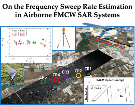
Graphical Abstract

1. Introduction

In the last years, an increasing interest toward Synthetic Aperture Radar (SAR) systems [1] mounted onboard aerial platforms, such as airplanes [2,3,4,5,6], helicopters [7], unmanned aerial vehicles (UAVs) [8,9] and drones [10,11], is registered [12]. This is mainly due to the high operative flexibility and relatively low operative costs of these platforms. Within this class of SAR systems, a key role is played by those based on the Frequency Modulated Continuous Wave (FMCW) technology [13]. Indeed, they operate with constant low transmission power, which implies simpler hardware, lower cost and smaller size than the pulse SAR systems [13].
To process FMCW SAR data, it is crucial to accurately know the radar Frequency Sweep Rate (FSR) [14]. Unfortunately, it may happen that the value of this electronic parameter, which is provided by the system supplier, is not sufficiently precise. In particular, use of an incorrect FSR value during the focusing procedure leads to an undesired stretching along the range direction of the final SAR image [15]. To overcome this problem, a method to estimate the FSR value actually used by the radar has been presented in [15]. The method is hereafter named FSR Estimate Through Corner reflectors (FSRETC), since it exploits in-situ measurements of the positions of a number of Corner Reflectors (CRs) deployed along the range direction of the illuminated area. Moreover, the method is based on the use of the SAR image focused with the available (erroneous) FSR, and thus affected by the geometric stretching effect mentioned above. In some extent, the available (erroneous) FSR represents the starting value that boots the overall estimation process, which is based on a linear model that relates proper observables (obtained through the measurements relevant to the CRs) to the true FSR value [15]. In [15] it is analytically shown that the accuracy of the FSRETC estimates can be improved in two ways. First, by increasing the number of CRs. Second, by spreading their positions along the range direction of the SAR image [15]. However, an experimental validation of this analysis misses in [15]. More generally, an experimental analysis on the robustness of the FSRETC algorithm with respect to variations of the number and positions of the used CRs misses. In [15] it is also remarked that for a generic FMCW SAR system one can think to apply the FSRETC algorithm only once, and to profitably use the estimated radar parameters to focus the data acquired during subsequent campaigns and missions. However, a validation experiment on this capability is missing [15]. More generally, an experimental analysis on the robustness over time of the FSRETC estimates is missing.
In this work, we provide an assessment of the capabilities of the FSRETC algorithm presented in [15]. In particular, we verify the robustness of the FSRETC algorithm with respect to the starting value of the FSR used to boot the estimation procedure. In addition, we verify the robustness of the FSRETC estimates with respect to variations of the number and positions of the used CRs. Moreover, we evaluate the performances achievable by the algorithm when exploiting repeat pass acquisitions over the same area. To do this, we exploit a dataset of 5 acquisitions carried out in the same day and over the same area considered in [15]. Furthermore, we consider also another dataset of 5 acquisitions carried out over the same area considered in [15], but 14 months later. In this way, on one side we analyze the robustness over time of the FSRETC estimates. On the other side, we pose the basis for an enhanced measurement strategy that allows effective application of the FSRETC algorithm through the use of only one CR. This strategy is indeed based on the use of a variety of radar acquisitions, spatially and temporally separated each-other, in substitution of the variety of CRs deployed over the illuminated area.
The work is organized as follows. In Section 2 we briefly recall the main rationale of the original algorithm in [15]. The experiments, all conducted with the Italian airborne FMCW AXIS InSAR system [16], are described in Section 3. The corresponding results are presented in Section 4 and discussed in Section 5. The concluding remarks are reported in Section 6.

2. Main Rationale of the FSRETC Algorithm

In this Section we briefly recall the main rationale of the FSRETC algorithm presented in [15].
The algorithm estimates two unknown electronic parameters of an FMCW SAR: the FSR, say α, and the uncompensated time delay, say μ, possibly occurring in the signal transmitted by the radar. Following the same notation introduced in [15], α ˜ denotes the incorrect available FSR. The two quantities α ˜ and α are related each other through the following relation:
α ˜ = α + ε
where ε is the constant unknown to be estimated along with the time delay μ.
Use of the incorrect FSR leads to the following range sampling step [15]:
δ ˜ R = c 2 α ˜ δ f
In Equation (2) the quantity δf is the true frequency resolution of the system. As can be seen, the quantity in Equation (2) is a scaled version of the true range sampling step, say δR, whose expression can be obtained substituting α ˜ with α in Equation (2). Use of the incorrect FSR during the focusing step produces an error in the target-to-radar distance measured by the radar [15]. In particular, by referring to a generic target, let us suppose that its true distance from the radar is R, whereas R ˜ is the distance erroneously measured by the radar. It can be shown [15] that the difference between these two quantities can be expressed as follows:
Δ R R R ˜ = R η ν
where
η ε α ˜ , ν c μ 2 α α ˜ = c μ 2 ( 1 η )
being c the light speed. As can be seen, the range difference Δ R in Equation (3) consists of two contributions. The quantity ν is independent of the radar-to-target distance: it is a bias that produces a rigid shift of the image along the range direction. The contribution , instead, depends on the true radar-to-target distance R and produces an image stretching along the range direction. It is also noted that Equation (3) is linear in the two unknowns ν and η, related to the unknown quantities ε and μ of our interest. Estimation of the two unknowns ν and η in Equation (3) requires that the quantities R and R ˜ , which are the observables of the linear model in Equation (3), are known at least in two different points of the observed area. One easy possibility to obtain such observables is to use CRs. More specifically, the quantity R relevant to the CRs can be obtained by measuring on one side the position of the CRs and on the other side the position of the radar antenna during the SAR acquisition. The former information can be obtained through in-situ measurements. The antenna position is provided by the navigation data collected onboard. The quantity R ˜ , still relevant to the CRs, can be instead obtained by exploiting the SAR image focused by using the available, erroneous, value of the FSR [15]. Indeed, the range coordinates of the imaged CRs correspond to the searched quantities R ˜ . It is remarked that for the purpose at hand the output grid used to focus the SAR image has to coincide with the radar grid. Summing up, once the quantities R and R ˜ are measured in correspondence of the two CRs, we can build and easily invert a linear system of two Equations in the form of Equation (3). From the estimated quantities ν and η we can then obtain the quantity ε in Equation (1) via Equation (4), thus achieving the desired estimate of the FSR actually employed by the radar.
It is stressed that the FSRETC algorithm requires to execute the SAR focusing procedure at least twice: first, by using the available incorrect FSR value α ˜ provided by the radar supplier (or any other value), and then, by correcting this value according to the obtained estimates (see [15] for more details). Hereafter, the quantity α ˜ is referred to as starting FSR; similarly, the SAR image used by the algorithm and obtained by using α ˜ is hereafter referred to as starting SAR image.
It is remarked that a number of CRs greater than two can be deployed in the illuminated area, thus obtaining an overdetermined system, whose inversion can be easily addressed through a Least Square (LS) approach [17]. In this regard, it is recalled that to improve the accuracy of the LS inversion, the number of used control points, which in our case are the CRs deployed over the illuminated area, has to be as large as possible [15]. Moreover, according to the theoretical analysis provided in [15], their positions must be well spread along the range direction of the SAR image. An experimental validation of this analysis however misses in [15].
In [15] it is also underlined that for a generic FMCW SAR system it is not necessary to apply the FSRETC algorithm before each flight campaign. Indeed, one can think to apply the algorithm only once, and to profitably use the estimated radar parameters to focus the data acquired by the system during subsequent campaigns and missions. However, an experimental validation of this potential capability misses in [15].

3. Experiments: Description and Aim

In order to assess the capabilities of the FSRETC algorithm, we have carried out a number of experiments by exploiting the data acquired during two flight campaigns carried out in 2018 and 2019, respectively, with an airborne FMCW SAR system named AXIS [16].
The system, which is based on the FMCW technology [13], consists of a radar module, three microstrip X-band antennas (one transmitting and two receiving) [18], an accurate Global Navigation Satellite System and an Inertial Measurement Unit (IMU). Thanks to the compactness and comparatively low weight of its components, the system can be mounted onboard small aircraft. For the experiments at hand, the system, whose main parameters are collected in Table 1, was mounted onboard a Cessna 172. Further details about AXIS can be found in [16].
The two flight campaigns considered for the experiments were conducted over the Salerno area, Italy. One campaign, consisting of 5 acquisitions (including the one considered in [15]) carried out in the same day, was performed in April 2018. The other campaign, still consisting of 5 acquisitions carried out in the same day, was performed in June 2019. All the 10 considered acquisitions have been planned over the same flight path, from South-East (SE) to North-West (NW). Of course, the unavoidable presence of atmospheric turbulences has induced deviations of the actually flown tracks from the planned path. For this reason, the flown tracks relevant to the 10 considered acquisitions are not coincident. Main acquisition parameters are summarized in Table 2.
Beside the flight campaigns, two ground campaigns (one in 2018, the other one in 2019) were conducted to deploy the CRs (5 in the 2018 and 5 in the 2019) over the area illuminated by the radar. The positions of the CRs were measured by means of Differential GPS (D-GPS) surveys. The CRs deployed during the two campaigns are highlighted in Figure 1 which reports, for each campaign, one amplitude SAR image (geocoded and superimposed over a Google Earth image) of the illuminated area. As can be seen (see left and right panels), the spatial distribution of the CRs is very similar in the two campaigns.
The description of the presented experiments is now addressed. In particular, the following 7 classes of experiments have been performed.
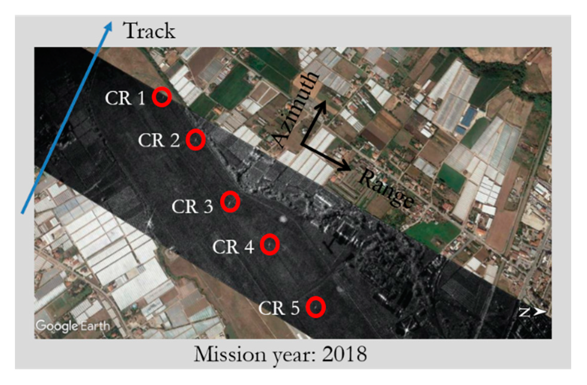
  • Experiments 1. The experiments are conducted with the same dataset considered in [15]. In particular, one acquisition (carried out in 2018) is considered. Moreover, 5 CRs are used for the estimate. With respect to [15], different starting FSR values are considered. In particular, in the experiments 1A, 1B, 1C three different starting FSR values are used. The experiment is aimed at assessing the robustness of the algorithm with respect to the starting FSR value used to boot the estimation procedure. The experimental scenario is summarized in Figure 2.
  • Experiments 2. Similarly to the Experiments 1, we have carried out three experiments, named 2A, 2B and 2C. The three experiments are conducted with the same dataset considered in the Experiments 1, using the same number of CRs (that is, 5). Moreover, the three starting FSR values of the experiments 1A, 1B and 1C, respectively, are used. With respect to the Experiments 1, the SAR image used for the estimation procedure is oversampled in the range direction. The experiments are aimed at verifying if range oversampling of the data improves the obtained estimates. The experimental scenario, equal to that of Experiment 1, is summarized in Figure 2 too.
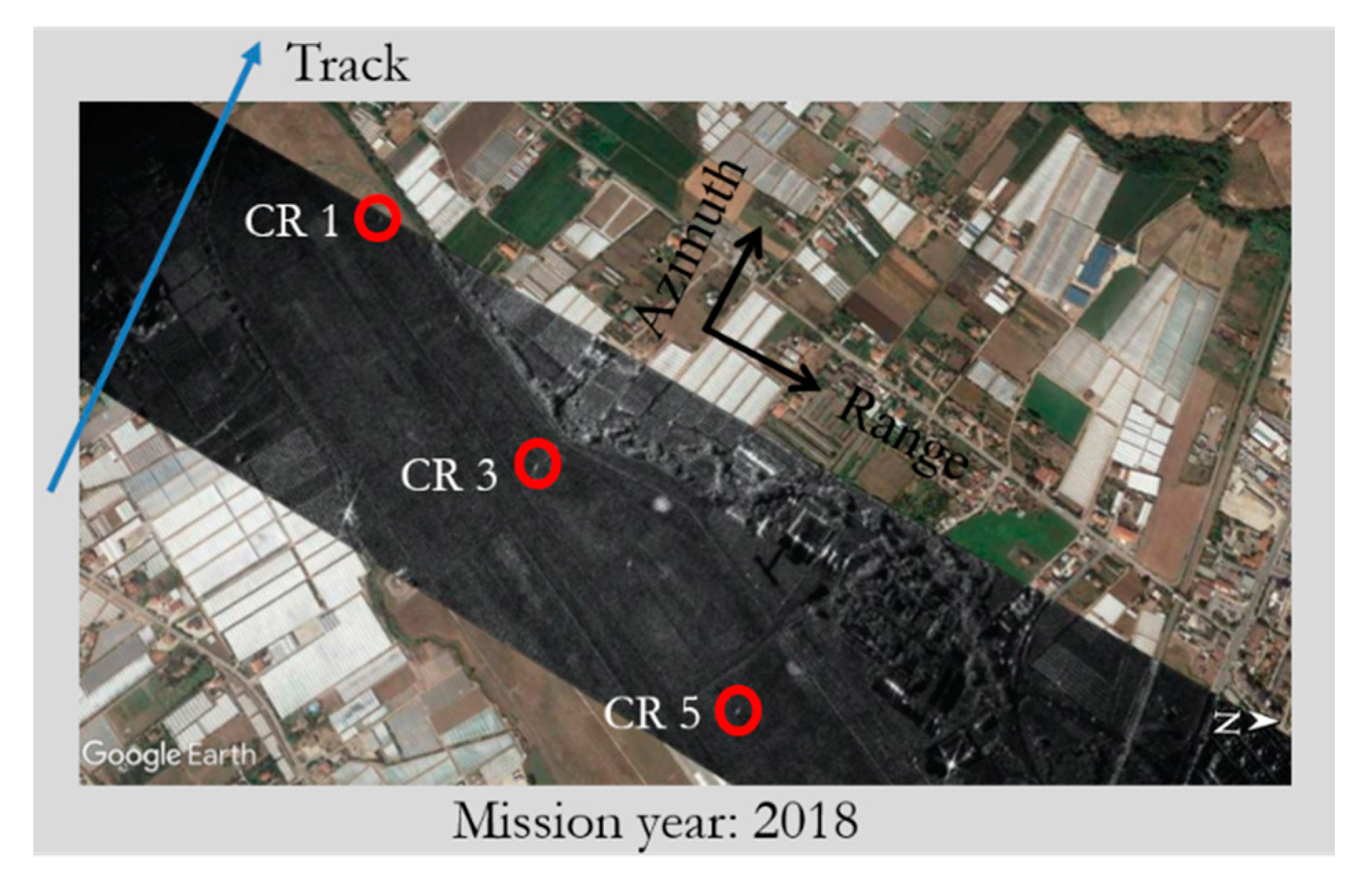
  • Experiment 3. The experiment is conducted with the same dataset considered in [15]. With respect to [15], a smaller number of CRs (that is, 3 rather than 5) are used for the estimation procedure. The experiment is aimed at verifying the robustness of the FSRETC algorithm with respect to variations of the number of CRs. The experimental scenario is summarized in Figure 3.
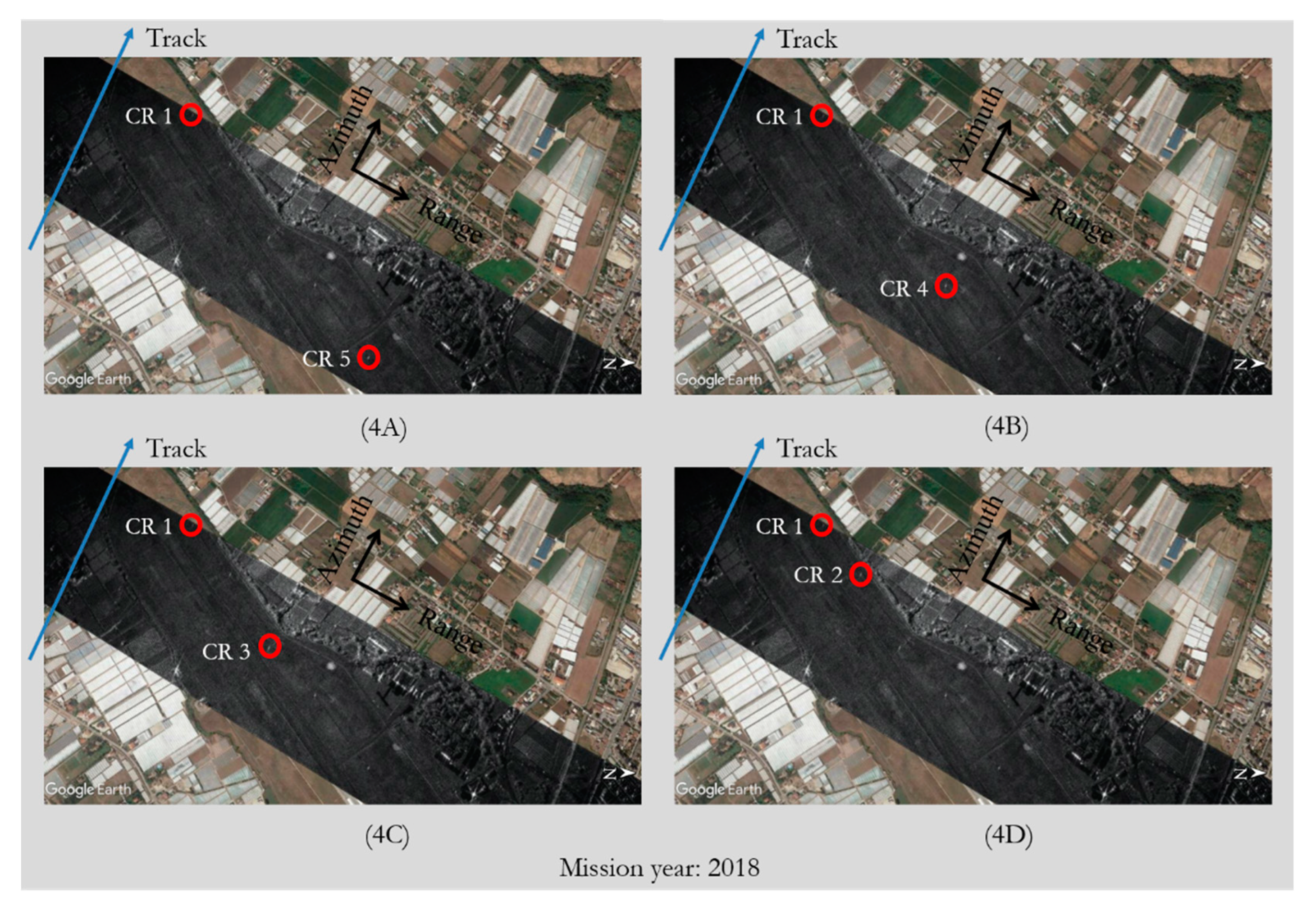
  • Experiments 4. The experiments are conducted with the same dataset considered in [15] and in the Experiment 3. With respect to the latter experiment, an even smaller number of CRs (that is, 2) are used for the estimation procedure. Moreover, in the experiments 4A, 4B, 4C and 4D we have progressively reduced the range distance between the two used CRs. More specifically, in these four experiments we have considered the following couples of CRs: CR1 and CR5, CR1 and CR4, CR1 and CR3, CR1 and CR2, respectively. The experiments are aimed at verifying the robustness of the FSRETC algorithm with respect to variations of number and positions of CRs. The experimental scenario of these experiments is summarized in Figure 4.
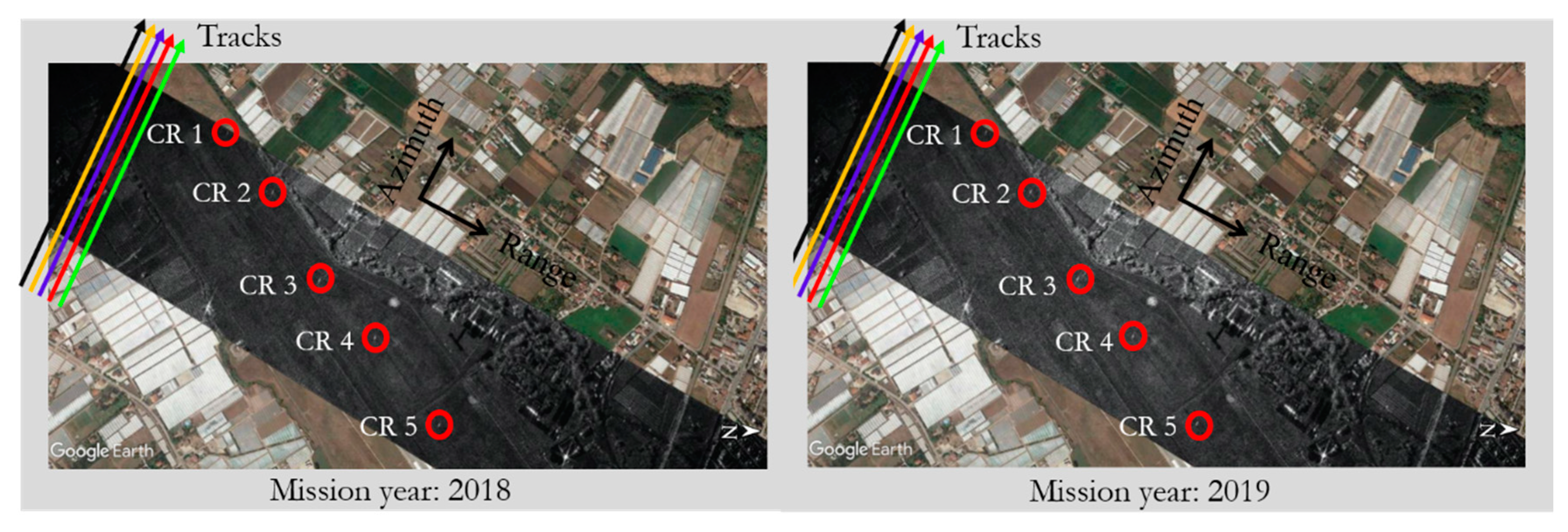
  • Experiment 5. The experiment is conducted with a dataset of 5 SAR acquisitions (including that considered in [15]) carried out in the same day and over the same area considered in [15]. The number of CRs used for the estimate is the same as that considered in [15], namely 5. The experiment is aimed at analyzing the robustness over time of the estimates provided by the FSRETC algorithm. The experimental scenario is summarized in Figure 5 (left panel).
  • Experiment 6. The experiment is conducted with a dataset of 5 SAR acquisitions carried out over the same area considered in [15], but 14 months later. The number of CRs used for the estimate is the same as that considered in [15] (that is, 5). The experiment is aimed at analyzing the robustness over time of the estimates provided by the FSRETC algorithm. The experimental scenario, which is equal to that of Experiment 5 apart from the dates of the acquisitions, is summarized in Figure 5 (right panel).
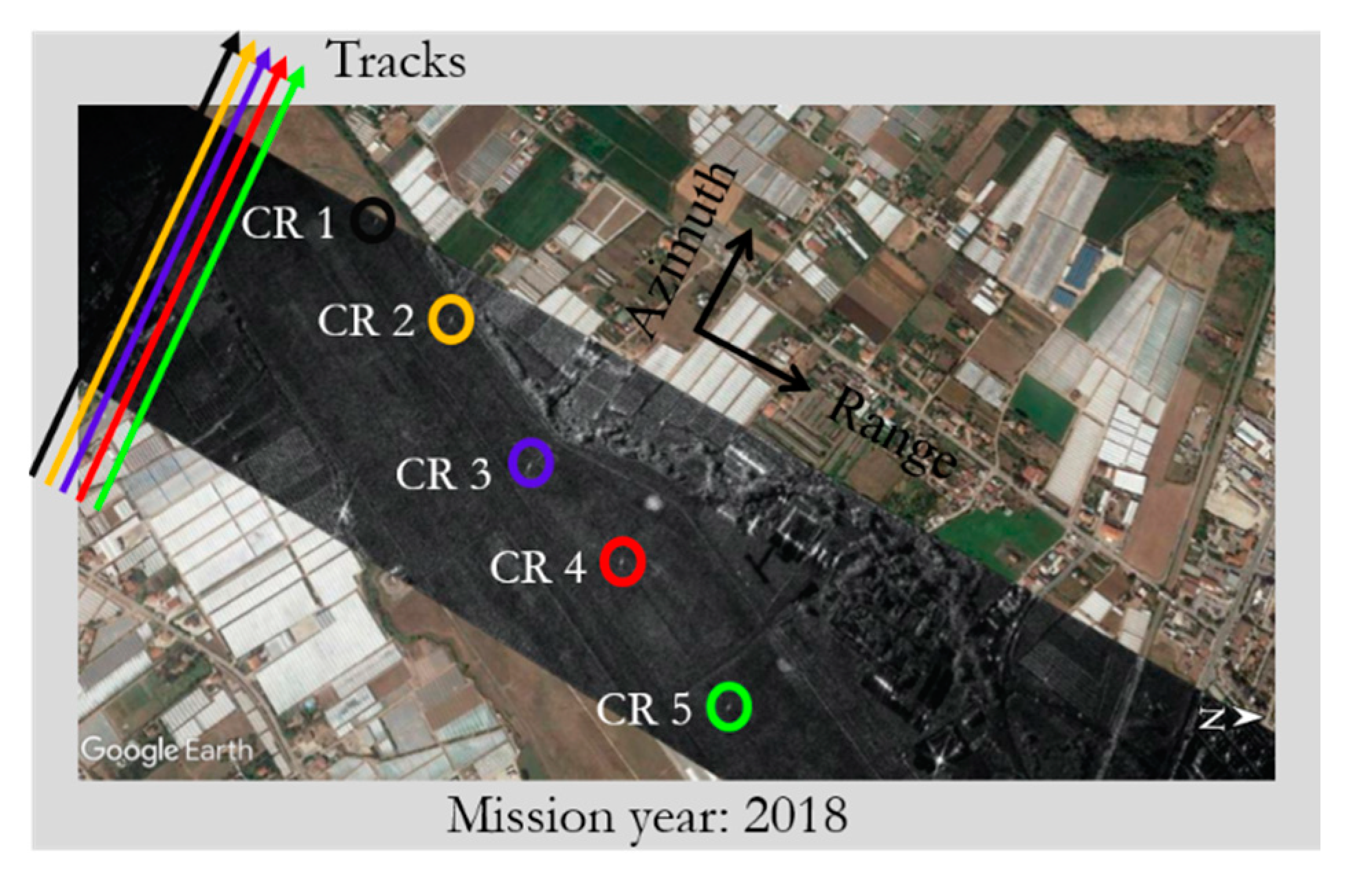
  • Experiment 7. The experiment is conducted with the same dataset considered in the Experiment 5. That is, five acquisitions (carried out in 2018) are considered. In contrast to the Experiment 5, for each acquisition we have considered only one CR. Notwithstanding, overall, all the 5 CRs are used for the estimate, since for each acquisition a different CR is considered. The experimental scenario is summarized in Figure 6, where the colors of the flight tracks and the circles show the correspondence between the acquisitions and the used CRs. In this way we simulate an acquisition scenario, not achievable with the available dataset, of 5 parallel flight paths in which only one CR is deployed on the observed area: through the different acquisitions the CR is illuminated from different view angles. The experiment is aimed at providing a preliminary evidence that the FSRETC algorithm can be successfully applied with only one CR by exploiting repeat pass acquisitions.

4. Experiments: Results

In this Section we present the results relevant to the 7 experiments described in Section 3. For the sake of clearness, the results are presented in 7 different Subsections, each of them relevant to a different experiment. Moreover, for comparison purposes we first recall the results obtained in [15], where it is used the same airborne SAR system considered in this work.
To focus the acquired data, the time-domain back projection technique [13,14,15,16,17,18,19] has been applied, by exploiting the information provided by the navigation data, the SRTM Digital Elevation Model [20] of the observed scene as well as the measurements of the antennas’ phase centers [18] and of the lever arms [16]. Moreover, a common output processing grid coincident to the radar grid relevant to the planned flight path, has been adopted. In particular, a 16 cm (azimuth) × 75 cm (range) grid sampling has been set. Moreover, the processing parameters have been set in such a way to achieve a geometric resolution of 35 cm (azimuth) × 75 cm (range).
The main results relevant to all the experiments are summarized in Table 3. Note in particular that for all the experiments we report in the table the starting FSR value α ˜ and the estimated one, say α ^ . Moreover, for the sake of clearness, the table collects also the starting range sampling step δ ^ R in Equation (2), and the estimated one, say δ ^ R , which can be obtained from Equation (2) by substituting α ˜ with α ^ . In Table 3 we have reported also a parameter, named Relative Range Stretching, briefly RRS, defined as follows:
R R S ( δ ^ R A δ ^ R B ) N r
where δ ^ R A and δ ^ R B are the range sampling steps estimated through two different experiments (indicated in table through the numbers within the brackets), and Nr is the number of range lines of the SAR data. The quantity in Equation (5) represents the overall geometrical stretching between two SAR images obtained with two different values of the FSR. We have introduced this figure of merit to quantify the effect of an erroneous FSR in the overall SAR image. As a rule of thumb, the estimates achieved through two experiments can be considered equivalent when the overall range stretching between the two corresponding SAR images is less than one range pixel. This implies that the following condition must be enforced:
| R R S | δ R R R S N < 1
For all the experiments, also the parameter RRSN in Equation (6), which represents the RRS normalized to the range sampling step, is reported in Table 3.
It is noted that from the condition in Equation (6) we can easily obtain (see Appendix A) the following upper limit for the accuracy, say Δα, required for the FSR estimate:
| Δ α | α < 1 N r
The condition in Equation (7) shows that the higher the overall number of range samples of the SAR data, the more accurate the estimate of the FSR must be.
Before analyzing in detail the results relevant to the 7 experiments described in Section 3, the results achieved in [15] are now briefly recalled. In [15], it is used the dataset relevant to one acquisition carried out in 2018: the experimental scenario is thus the same as that depicted in Figure 2. The starting FSR value used in [15] to boot the estimation procedure is reported in Table 3. After application of the FSRETC algorithm, the mean misalignment between the actual CRs’ positions and those calculated in the focused SAR image is equal to 26 cm, which is about one third of the range resolution of the system. The main results relevant to this experiment represent our reference estimates for comparisons with the results of the subsequent experiments. As clarified above, the results relevant to the 7 experiments described in Section 3 are presented in the following 7 subsections.

4.1. Experiments 1

In the Experiments 1, three starting FSR values different from that used in [15] are exploited to boot the estimation procedure, see Table 3. In particular, in the Experiment 1A, with respect to [15], we have used an updated value, say FSRc, still provided by the radar supplier according to lab measurements independent of our experiments. We have then considered a 2% tolerance interval, say [FSRl, FSRu], around FSRc. Note that this interval includes the previous FSR value provided by the radar supplier and used in [15] as starting value. In the Experiments 1B and 1C we have used FSRl and FSRu, respectively, as starting FSR values.
From the results collected in Table 3, we can observe that the differences between the range sampling step δ ^ R obtained in [15] and with the Experiment 1A lead to RRSN = 0.4. Therefore, the results obtained in these cases can be considered equivalent. Moreover, the differences between the estimates achieved through the Experiments 1C and 1A lead to RRSN = 1.1. The condition (6) is thus almost fulfilled. Accordingly, using as starting FSR the central value FSRc or the upper limit FSRu of the considered tolerance interval leads practically to the same result. Unfortunately, similar considerations do not hold when we consider as starting FSR the lower limit FSRl. Indeed, the differences between the estimates achieved through the Experiments 1B and 1A lead to RRSN = 4.6 pixels. However, as shown in the next Subsection, this poor result can be significantly improved by performing a range oversampling of the starting SAR image exploited by the algorithm.

4.2. Experiments 2

In the Experiments 2A, 2B and 2C we have used the three starting FSR values of the experiments 1A, 1B and 1C, respectively. Differently from the Experiments 1, we have performed a range oversampling of the starting SAR image exploited by the algorithm. More specifically, we have applied a zero-padding procedure in the frequency domain. From the results collected in Table 3, we can observe that in this case, using as starting FSR the central value FSRc, the lower limit FSRl or the upper limit FSRu of the considered tolerance interval leads always practically to the same result. Indeed, the differences between the estimates achieved through the Experiments 2B and 2A lead to RRSN = 0.2. Similarly, the differences between the estimates achieved through the Experiments 2C and 2A lead to RRSN = 0.2. From these results it turns that the performed range oversampling makes the algorithm robust with respect to variations of the starting FSR value used to boot the overall estimation procedure.
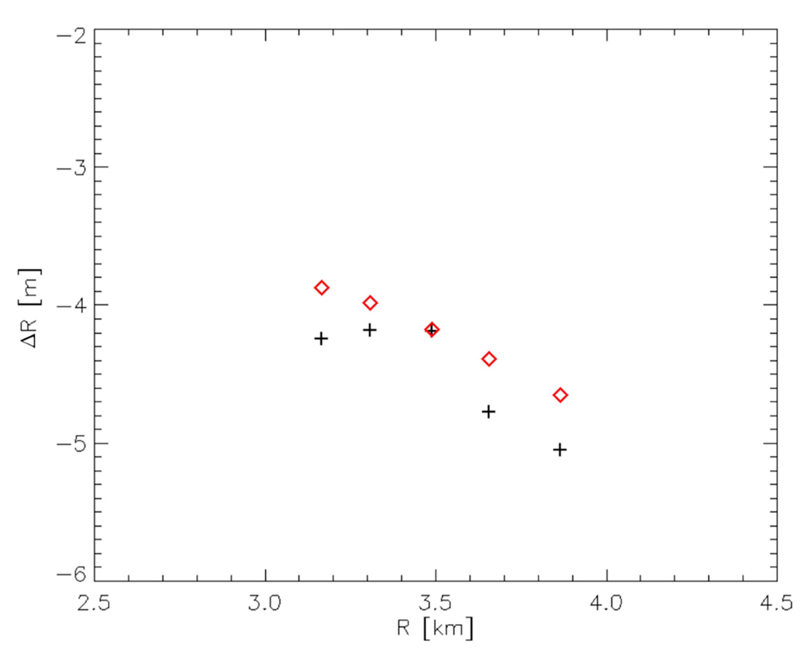
To better investigate the effects of this oversampling procedure on the estimation process, let us focus on the Experiments 2A and refer to Equation (3). With the applied oversampling, for each considered CR we have retained the same value of R (which is independent of the image) considered in the Experiment 1A, but we have obtained a different value for R ˜ , and thus for the quantity ΔR used by the estimation algorithm. The different values ΔR used in the Experiments 1A and 2A are plotted in Figure 7 as a function of the true CR-to-radar distance R. As can be seen, the differences are quite small, and in any case less than the range resolution of the system. On the other side, it is also noted that the range oversampling of the starting SAR image allows to better recover the expected linear relationship in (3) between the quantities ΔR and R. Accordingly, a better matching between the inversion model and the used observables is obtained. Therefore, we can safely conclude that the observables obtained by oversampling the starting SAR image are more reliable for the estimate. For this reason, the estimates achieved in the Experiments 2 are more stable than those obtained in the Experiments 1.
In all the subsequent experiments, to obtain measurements able to better match the inversion model of the FSRETC algorithm, the starting SAR image used by the algorithm is always oversampled as in the Experiments 2. Moreover, in all the subsequent experiments, for the sake of fairness, we have always considered the starting FSR value adopted in the Experiments 1A and 2A.

4.3. Experiment 3

In the Experiment 3 we have verified the robustness of the FSRETC algorithm with respect to variations of the number of CRs. In particular, we have applied the algorithm by using the information relevant to only three CRs, namely CR1, CR3 and CR5. Note that we have selected these three CRs in such a way that they cover (obviously with less spatial density) the same range extent achieved with all the 5 CRs (see Figure 2; Figure 3).
From the results collected in Table 3, we can observe that the quantities estimated through the Experiments 2A and 3 are very similar. In particular, the differences between the corresponding range sampling step values δ ^ R lead to RRSN = 0.2, which is smaller than one pixel. From this result we can draw the conclusion that when passing from 5 CRs to 3 CRs, the accuracy of the estimates does not change significantly, at least when the positions of the 3 CRs cover the same range extent of the 5 CRs.

4.4. Experiments 4

In the Experiments 4 we have verified the robustness of the estimates provided by the FSRETC algorithm with respect to variations of the number and the positions of the used CRs. In particular, we have used only two CRs, thus reducing even more the number of CRs considered in the Experiment 3. Moreover, we have carried out four different experiments by gradually reducing the range distance between the two used CRs. More specifically, in the Experiment 4A, we have used CR1 and CR5. These two CRs have been thus selected according to the same rationale adopted for the Experiment 3 (see Experiment 4A in Figure 4A). From the results collected in Table 3, we can observe that also in this case (as in the previous Experiment 3) the estimated quantity is very close to that achieved in the Experiment 2A. In particular, the differences between the corresponding range sampling step values δ ^ R estimated through the Experiments 2A and 4A lead to RRSN = 0.2, which is much smaller than one pixel. From this result we can draw the conclusion that when passing from 5 CRs to 2 CRs, the accuracy of the estimates of the algorithm does not change significantly, at least when the positions of the 2 CRs cover the same range extent of the 5 CRs.
We have then gradually reduced the range distance between the two used CRs. In particular, as shown in the different panels of Figure 4, in the Experiments 4B, 4C and 4D we have considered the following couples of CRs: CR1 and CR4, CR1 and CR3, CR1 and CR2, respectively. From the obtained results (reported as usual in Table 3) we can observe that the smaller the range extent covered by the 2 CRs the worse the accuracy of the estimated quantities. In particular, the differences between the corresponding range sampling step values δ ^ R estimated through the Experiments 4B, 4C and 4D and the Experiment 2A lead to RRSN = 0.6, 1.5, 2.9, respectively. From these results we draw the conclusion that when passing from 5 CRs to 2 CRs, it is recommended to keep the range extent covered by the couple of CRs as large as possible. This is in agreement with the theoretical analysis presented in [15]. In the case at hand, a (slant) range separation of about 500 m (Experiment 4B) is enough to obtain a sufficiently accurate estimate of the searched FSR. Indeed, from the estimates obtained in the Experiments 4B and 2A we obtain RRSN less than one pixel.

4.5. Experiment 5

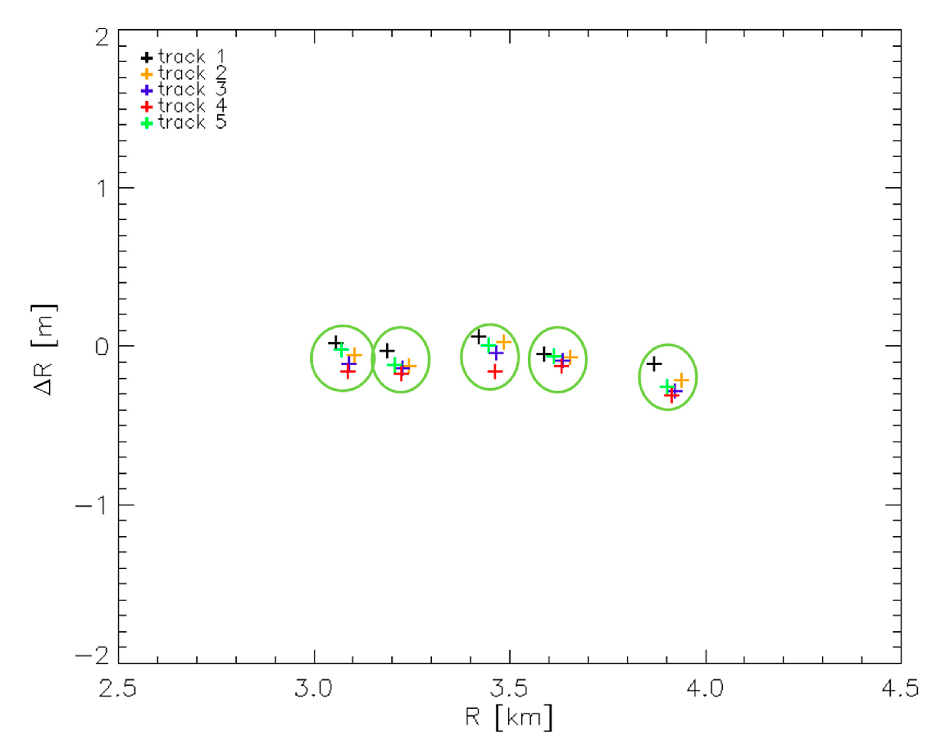
The Experiment 5 is aimed at analyzing the robustness over time of the estimates provided by the algorithm. To do this, we have considered 5 repeat pass acquisitions (including the one considered in the previous experiments) carried out in April 2018, all in the same day. For all the acquisitions, we used all the 5 CRs. In this way we obtained a number of measurements significantly higher than that used in all the experiments considered so far. In particular, in this case we have collected a set of 25 measurements (5 for each acquisition), against the 5 measurements exploited in [15] and in the Experiments 1 and 2, the 3 measurements exploited in the Experiment 3, and the 2 measurements exploited in the Experiments 4. The 25 different values ΔR used by the FSRETC algorithm in the Experiment 5 are plotted in Figure 8, as a function of the true CR-to-radar distances R. In the figure, each green circle groups the same CR in the five different acquisitions. In each circle we can observe a spreading of the measurement results in the horizontal and vertical directions. The presence of the horizontal spreading shows that in the different acquisitions to the same CR correspond to different values of the CR-to-radar distance R. This is due to the fact that the 5 considered flight tracks are not coincident. Indeed, as highlighted above, they are characterized by different track deviations from the planned flight path. Furthermore, they are characterized by different squint angles. The vertical spreading is instead an index of the repeatability over time (at least, during the same day) of the measurements exploited by the algorithm to obtain the estimates. No spreading (or better, a very marginal linear variation due to the variation of the CR-to-radar distances in the different acquisitions, see Equation (3)) is indeed expected along the vertical axis within each circle. The amount of the vertical and horizontal spreading of the measurement results plotted in Figure 8 is quantified in Table 4 (first line), which reports, for each CR, the standard deviation of the quantities ΔR (vertical spreading) and R (horizontal spreading) measured before application of the FSRETC algorithm. From Table 4 and the plot of Figure 8 we can appreciate that the vertical spreading of the measurements is, for all the considered CRs, always less than the range resolution of the system. This indicates a very good repeatability over time (at least, during the same day) of the measurements exploited by the algorithm to obtain the estimates. Such a good repeatability is confirmed by the obtained estimates, reported as usual in Table 3. As can be seen, the results obtained in the Experiment 5 are very close to those reached in the Experiment 2A, that is, the overall estimation process is not impaired when using different SAR acquisitions temporally separated. In particular, from the two values δ ^ R obtained in the Experiment 5 and 2A we obtain RRSN = 1.1. The condition (6) is thus almost fulfilled. To better appreciate the accuracy of the obtained results, we have focused all the 5 SAR images by exploiting the FSR estimated with this experiment. Then, we have applied once again the FSRETC algorithm: the 25 different values ΔR measured in this case are plotted in Figure 9, as usual as a function of the true CR-to-radar distances R. Again, in the figure each green circle groups the same CR in the five different acquisitions. As can be seen and expected, the linear trend of ΔR with respect to the radar-to-target distances R, clearly visible in Figure 8 due to the use of an erroneous FSR during the focusing step (see Equations (3)–(4)), disappears in Figure 9. For the sake of completeness, in Table 4 (second line) for each CR we report also the standard deviation of the quantities ΔR (vertical spreading) and R (horizontal spreading) measured after application of the FSRETC algorithm.

4.6. Experiment 6

In the Experiment 6 we have replaced the Experiment 5, but considering 5 acquisitions carried out in June 2019 (and not April 2018 as in the Experiment 5), all in the same day. The 25 different values ΔR used by the FSRETC algorithm in this case are plotted in Figure 10. As in Figure 8, also in this case each green circle groups the same CR in the five different acquisitions. For this plot we can repeat the same considerations carried out above for the plot of Figure 8 relevant to the 2018 dataset. In this case we just observe a more noticeable vertical spreading of the measurements relevant to the CRs located in far range. As usual, in Table 4 for each CR we report the standard deviation of the quantities ΔR (vertical spreading) and R (horizontal spreading) measured before and after application of the FSRETC algorithm.
Note in particular that the amount of the observed vertical spreading (before and after application of the FSRETC algorithm) is less than the range resolution of the system. In addition, it is remarked that the results obtained in this experiment and in the Experiment 5 are very similar (see Table 3): the difference between the two values δ ^ R obtained in the two experiments lead to RRSN = 0.6, which once again is smaller than 1. This confirms a very good repeatability over a time span of 14 months of the measurements exploited by the algorithm to obtain the estimates. Also in this case, to better appreciate the accuracy of the obtained estimates, we have focused all the 5 SAR images by exploiting the FSR estimated with this experiment, and repeated the procedure leading to the plot of Figure 9. The obtained results are plotted in Figure 11: also in this case, as expected, the linear trend of ΔR with respect to the radar-to-target distances R disappears.

4.7. Experiment 7

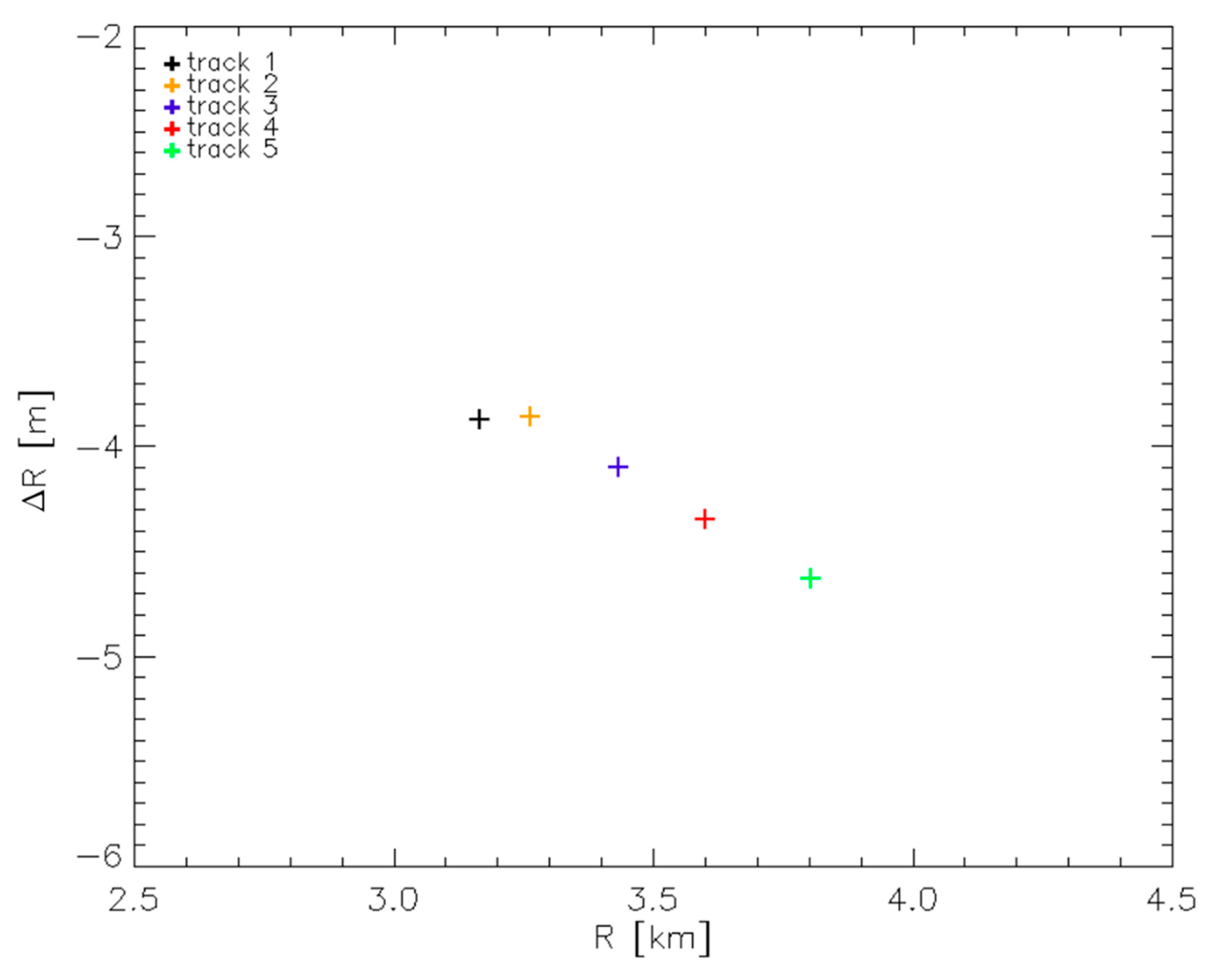
In the Experiment 7 we have used the same repeat pass dataset considered in the Experiment 5, that is, relevant to the 5 acquisitions of April 2018. In particular, for each acquisition we have considered only one CR. The 5 CRs considered in the 5 different acquisitions are different each other. By doing so, we have collected, similarly to the Experiments 1 and 2, a set of 5 measurements (1 for each acquisition), against the 25 used in the Experiment 5. The 5 different values ΔR used by the FSRETC algorithm in this Experiment 7 are plotted in Figure 12, as a function of the true CR-to-radar distances R. In the figure, each color denotes a different CR as well as a different acquisition. In other words, although using 5 different CRs and 5 almost coincident flight paths, we have simulated a scenario of 5 parallel flight paths in which only one CR is deployed on the observed area, and through the different acquisitions the CR is illuminated from different view angles. As can be seen (see Table 3) the results obtained in the Experiment 7 and 2A (which exploit the same number of measurements, obtained however with 5 and 1 radar acquisitions, respectively) are very similar: the difference between the two values δ ^ R obtained in the two experiments lead to RRSN = 1.
It is finally noted that in all the considered experiments (with the exceptions of Experiments 1B and 4D), the estimated constant bias ν ^ in (3) is on the order of the range resolution of the system (see again Table 3).

5. Discussion

In the previous Sections we have presented a number of experiments aimed at assessing the capabilities of the FSRETC algorithm.
In particular, the Experiments 1 and Experiments 2 have shown that the estimates provided by the algorithm are independent of the starting FSR used to boot the estimation procedure, provided that proper range oversampling of the starting SAR image is applied. More generally, the Experiments 2 have shown that the range oversampling of the SAR image used by the algorithm is convenient, since it allows to better recover the expected linear relationship between the quantities ΔR and R, which represent the observables of the linear model in (3) exploited by the FSRETC algorithm.
The Experiments 3 and 4 have shown that reducing the number of CRs with respect to the experiment in [15] does not produce an appreciable degradation of the accuracy of the obtained estimates. In particular, when passing from the 5 CRs of the experiment in [15] to the 2 CRs of the Experiments 4, the estimates provided by the FSRETC algorithm are practically the same, at least when the 2 CRs are deployed in such a way to cover a range extent similar to that covered by the 5 CRs. More specifically, the Experiments 4 have shown that when using only two CRs, it is essential to keep as large as possible the range extent covered by the CRs positions. Overall, the results achieved through the Experiments 4 provide a very useful indication to save costs and time for the calibration of new-borne airborne FMCW SAR systems.
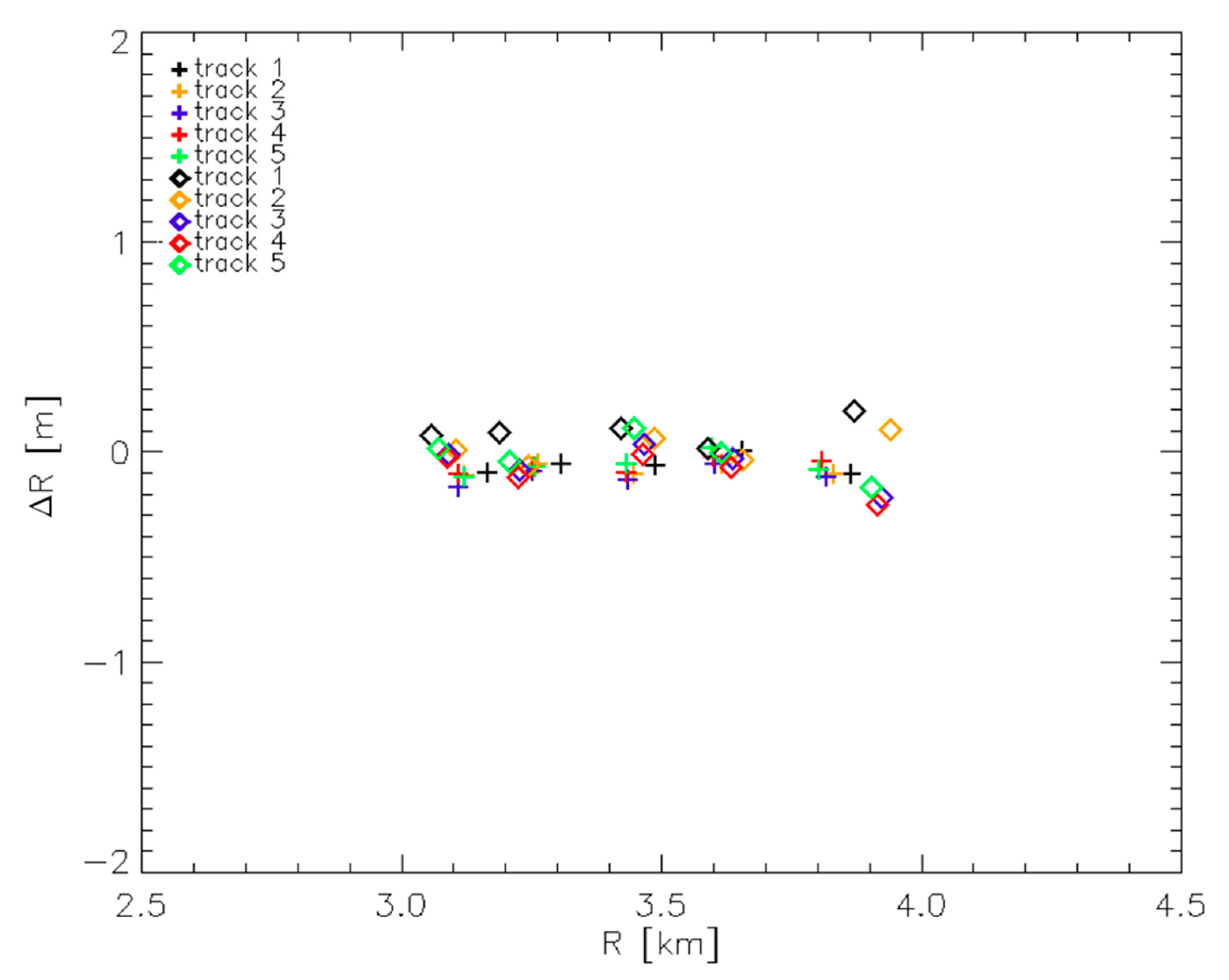
The Experiment 5 has shown that when the different acquisitions are carried out in the same day, a very good repeatability of the measurements exploited by the algorithm is achieved over time. Moreover, comparison between the results of the Experiments 5 and 6 has shown a very good repeatability over a time span of 14 months of the estimates achieved through the FSRETC algorithm. Accordingly, we can conclude that, at least for the considered SAR system, the algorithm can be safely applied only once, since the estimated FSR turns out very stable at least over a time span of 14 months. This means that this estimated value can be profitably used to focus the data acquired by the system during subsequent campaigns and missions. To better show this, we have focused all the 10 SAR images relevant to the two datasets acquired in April 2018 and June 2019 by exploiting the FSR estimated with the Experiment 5 (that is, by using all the acquisitions of April 2018 and all the CRs). Then, we have applied once again the FSRETC algorithm: the 50 different values ΔR measured in this case are plotted in Figure 13, as usual as a function of the true CR-to-radar distances R. As can be seen, the linear trend of ΔR with respect to the radar-to-target distances R (due to the use of an erroneous FSR during the focusing step) disappears in the measurements relevant to the both the year 2018 (as already shown in Figure 9) and the year 2019, represented in the figure by crosses and diamonds, respectively. For the 2019 dataset, we just observe a more noticeable vertical spreading of the measurements relevant to the far range CRs; in any case, the amount of this effect, which is quantified as usual in Table 4, is less than the range resolution of the system. Summing up, the plot of Figure 13 shows that the estimate obtained by exploiting the dataset acquired in April 2018 could have been safely used also in June 2019, without calibrating the system once again by deploying the CRs, measuring their positions and applying the FSRETC algorithm again.
In this regard, we observe that the stability over time of the measurements exploited by the algorithm (leading to the stability over time of the obtained estimates) represents a very attractive feature that can be profitably exploited to reduce even more the number of the used CRs, without reducing the number of ground control points exploited by the FSRETC algorithm. Indeed, we can think to deploy only one CR and exploit repeat pass SAR acquisitions along parallel tracks so as to illuminate the CR from different view angles. To validate such approach, a proper dataset would be necessary. Unfortunately, all the SAR acquisitions at our disposal are relevant to the same nominal flight path. Moreover, even considering the unavoidable deviations affecting the actually flown tracks, each CR is illuminated by the different tracks practically with the same view angle. To show the potentialities of this approach based on the use of only one CR, we have carried out the Experiment 7, which emulates with the available dataset a virtual acquisition scenario consisting of parallel tracks. The obtained results pose the basis for an enhanced measurement strategy (to be validated in the very next future through an ad-hoc acquisition campaign) which guarantees the spatial spreading of the ground control points exploited by the FSRETC algorithm through a variety of radar acquisitions, spatially and temporally separated each-other, in substitution of the variety of CRs deployed over the illuminated area.

6. Conclusions and Future Developments

In this work, we have assessed the robustness of the FSRETC algorithm proposed in [15] to estimate the FSR value actually employed by a FMCW SAR. To do this, starting from the same experiment presented in [15] we have carried out a number of experiments through the use of airborne SAR data acquired by the same system considered in [15].
The presented results show that the algorithm is robust with respect to the starting FSR chosen to boot the estimation procedure, provided that proper range oversampling of the SAR image exploited by the algorithm is performed. Moreover, even with a single acquisition, use of only two CRs, sufficiently far from each other in the range direction, allows achieving an accurate estimate of the searched FSR. The presented experiments show also that the estimate obtained with the algorithm is stable over the time interval considered in the work, that is, 14 months. Accordingly, at least for the considered SAR system, the FSRETC algorithm can be applied only once, and the estimated FSR can be safely used to focus the data acquired by the system during subsequent campaigns and missions.
The presented results, in addition to providing an assessment of the capabilities of the FSRETC algorithm, pose the basis for an enhanced measurement strategy capable of reducing to only one the number of CRs necessary to apply the algorithm. Indeed, by taking advantage from the stability over time of the estimates obtained through the algorithm, one can increase the number of ground measurements by exploiting a variety of radar acquisitions, spatially and temporally separated each-other, in substitution of the variety of CRs deployed over the illuminated area. Although full validation of such approach would require an ad-hoc acquisition campaign consisting of repeat pass SAR acquisitions along parallel tracks, a preliminary promising validation result has been presented in the work by exploiting repeat pass acquisitions all planned along the same path.

Author Contributions

Conceptualization, C.E., P.B., S.P.; Methodology, Software and Validation, C.E., A.N., P.B., S.P.; Investigation, C.E., P.B., S.P.; Data Curation, C.E., A.N., P.B., S.P.; Writing-Original Draft Preparation, C.E., S.P.; Supervision, S.P. All authors have read and agreed to the published version of the manuscript.

Funding

The work has been supported in part by the Italian Department of Civil Protection (DPC) in the framework of DPC-IREA Agreement (2019–2021) and in part by the Italian Ministry of Economic Development (MISE) in the framework of the contract “MATRAKA”. Part of the presented research has been carried out through the I-AMICA (Infrastructure of High Technology for Environmental and Climate Monitoring-PONa3_00363).

Acknowledgments

The authors thank Elettra Microwave srl and Etabeta srl for their support during the acquisition and ground campaigns. They also thank the anonymous reviewers for their careful review and for their useful comments and suggestions.

Conflicts of Interest

The authors declare no conflict of interest.

Appendix A

In this appendix we derive condition in Equation (7). To this aim, let us consider an FSR estimate, say α ^   =   α + Δ α , leading to the range sampling step δ ^ R . Following the formalism introduced in Equation (1), α is the true FSR whereas Δα represents the estimation error. Let us now rewrite the RRS in Equation (5) by substituting the quantities δ ^ R A and δ ^ R B with the true range sampling step δR and δ ^ R , respectively. By doing so, the RRS in Equation (5) can be written as follows:
R R S = ( δ R δ ^ R ) N r = R f a r R ^ f a r = R f a r Δ α α ^
where R f a r is the true far range whereas R ^ f a r is the far range obtained according to the estimated FSR range sampling step. Moreover, in the last equality we have used Equations (3)–(4), provided that R ˜ in Equation (3) is substituted by R ^ f a r , the error ε in Equation (4) is substituted by the estimation error Δα and the bias μ in Equation (4) (which is of no interest for this discussion) is zero. Substitution of Equation (A1) in Equation (6) leads to:
| R R S | δ R = R f a r δ R | Δ α | α ^ = N r | Δ α | α ^ < 1
When the number Nr of range samples is much larger than 1, as it always happens in all the practical cases, the condition in Equation (A2) becomes equivalent to that in Equation (7).

References

  1. Franceschetti, G.; Lanari, R. Synthetic Aperture Radar Processing; CRC Press: Boca Raton, FL, USA, 2018; ISBN 9781351412018. [Google Scholar]
  2. Perna, S.; Esposito, C.; Amaral, T.; Berardino, P.; Jackson, G.; Moreira, J.; Pauciullo, A.; Junior, E.V.; Wimmer, C.; Lanari, R. The InSAeS4 airborne X-band interferometric SAR system: A first assessment on its imaging and topographic mapping capabilities. Remote Sens. 2016, 8, 40. [Google Scholar] [CrossRef] [Green Version]
  3. Magnard, C.; Frioud, M.; Small, D.; Brehm, T.; Essen, H.; Meier, E. Processing of MEMPHIS Ka-band multibaseline interferometric SAR data: From raw data to digital surface models. IEEE J. Sel. Top. Appl. Earth Obs. Remote Sens. 2014, 7, 2927–2941. [Google Scholar] [CrossRef]
  4. Pinheiro, M.; Reigber, A.; Scheiber, R.; Prats-Iraola, P.; Moreira, A. Generation of highly accurate DEMs over flat areas by means of dual-frequency and dual-baseline airborne SAR interferometry. IEEE Trans. Geosci. Remote Sens. 2018, 56, 4361–4390. [Google Scholar] [CrossRef] [Green Version]
  5. Pinheiro, M.; Amao-Oliva, J.; Scheiber, R.; Jaeger, M.; Horn, R.; Keller, M.; Fischer, J.; Reigber, A. Dual-Frequency Airborne SAR for Large Scale Mapping of Tidal Flats. Remote Sens. 2020, 12, 1827. [Google Scholar] [CrossRef]
  6. Du Plessis, O.R.; Nouvel, J.F.; Baqué, R.; Bonin, G.; Dreuillet, P.; Coulombeix, C.; Oriot, H. ONERA SAR facilities. IEEE Aerosp. Electron. Syst. Mag. 2011, 26, 24–30. [Google Scholar] [CrossRef]
  7. Perna, S.; Alberti, G.; Berardino, P.; Bruzzone, L.; Califano, D.; Catapano, I.; Ciofaniello, L.; Donini, E.; Esposito, C.; Facchinetti, C.; et al. The ASI integrated sounder-SAR system operating in the UHF-VHF bands: First results of the 2018 helicopter-borne morocco desert campaign. Remote Sens. 2019, 11, 1845. [Google Scholar] [CrossRef] [Green Version]
  8. Aguasca, A.; Acevo-Herrera, R.; Broquetas, A.; Mallorqui, J.J.; Fabregas, X. ARBRES: Light-weight CW/FM SAR sensors for small UAVs. Sensors 2013, 13, 3204–3216. [Google Scholar] [CrossRef] [PubMed] [Green Version]
  9. Rosen, P.A.; Hensley, S.; Wheeler, K.; Sadowy, G.; Miller, T.; Shaffer, S.; Muellerschoen, R.; Jones, C.; Madsen, S.; Zebker, H. UAVSAR: New NASA Airborne SAR System for Research. IEEE Aerosp. Electron. Syst. Mag. 2007, 22, 21–28. [Google Scholar] [CrossRef]
  10. Oré, G.; Alcântara, M.S.; Góes, J.A.; Oliveira, L.P.; Yepes, J.; Teruel, B.; Castro, V.; Bins, L.S.; Castro, F.; Luebeck, D.; et al. Crop growth monitoring with drone-borne DInSAR. Remote Sens. 2020, 12, 615. [Google Scholar] [CrossRef] [Green Version]
  11. Luebeck, D.; Wimmer, C.; Moreira, L.F.; Alcântara, M.; Oré, G.; Góes, J.A.; Oliveira, L.P.; Teruel, B.; Bins, L.S.; Gabrielli, L.H.; et al. Drone-borne differential SAR interferometry. Remote Sens. 2020, 12, 778. [Google Scholar] [CrossRef] [Green Version]
  12. Perna, S.; Soldovieri, F.; Amin, M. Editorial for special issue “radar imaging in challenging scenarios from smart and flexible platforms”. Remote Sens. 2020, 12, 1272. [Google Scholar] [CrossRef] [Green Version]
  13. Richards, M.A.; Scheer, J.A.; Holm, W.A. Principles of Modern Radar: Basic Principles; Scitech Publishing: Raleigh, NC, USA, 2010; ISBN 9781613531488. [Google Scholar]
  14. Meta, A.; Hoogeboom, P.; Ligthart, L.P. Signal processing for FMCW SAR. IEEE Trans. Geosci. Remote Sens. 2007, 45, 3519–3532. [Google Scholar] [CrossRef]
  15. Esposito, C.; Natale, A.; Palmese, G.; Berardino, P.; Perna, S. Geometric distortions in FMCW SAR images due to inaccurate knowledge of electronic radar parameters: Analysis and correction by means of corner reflectors. Remote Sens. Environ. 2019, 232, 111289. [Google Scholar] [CrossRef]
  16. Esposito, C.; Natale, A.; Palmese, G.; Berardino, P.; Lanari, R.; Perna, S. On the Capabilities of the Italian Airborne FMCW AXIS InSAR System. Remote Sens. 2020, 12, 539. [Google Scholar] [CrossRef] [Green Version]
  17. Kay, S.M. Kay Fundamentals of Statistical Signal Processing: Estimation Theory; Prentice-Hall, Inc., Division of Simon and Schuster One Lake Street: Upper Saddle River, NJ, USA, 1993. [Google Scholar]
  18. Esposito, C.; Gifuni, A.; Perna, S. Measurement of the Antenna Phase Center Position in Anechoic Chamber. IEEE Antennas Wirel. Propag. Lett. 2018, 17, 2183–2187. [Google Scholar] [CrossRef]
  19. Berardino, P.; Esposito, C.; Natale, A.; Lanari, R.; Perna, S. Airborne SAR Focusing in the Presence of Severe Squint Variations. In Proceedings of the IGARSS 2019—2019 IEEE International Geoscience and Remote Sensing Symposium, Yokohama, Japan, 28 July–2 August 2019. [Google Scholar]
  20. Rabus, B.; Eineder, M.; Roth, A.; Bamler, R. The shuttle radar topography mission—A new class of digital elevation models acquired by spaceborne radar. ISPRS J. Photogramm. Remote Sens. 2003, 57, 241–262. [Google Scholar] [CrossRef]
Figure 1. Multi-look amplitude SAR image (in geographic grid) patch of the entire acquired strip. The green circles indicate the CRs’ positions. Left: relevant to the 2018 campaign. Right: relevant to the 2019 campaign.
Remotesensing 12 03448 g001
Figure 2. Relevant to the Experiments 1 and the Experiments 2. As Figure 1, with highlighted the CRs and (a pictorial view of) the tracks exploited in these experiments. Number of exploited CRs (red circles): 5. Number of exploited tracks (blue line): 1. Mission year: 2018.
Remotesensing 12 03448 g002
Figure 3. As Figure 2, but relevant to the Experiment 3. Number of exploited CRs (red circles): 3. Number of exploited tracks (blue line): 1. Mission year: 2018.
Remotesensing 12 03448 g003
Figure 4. As Figure 2, but relevant to the Experiment 4A (A), Experiment 4B (B), Experiment 4C (C) and Experiment 4D (D). Number of exploited CRs (red circles): 2. Number of exploited tracks (blue line): 1. Mission year: 2018.
Remotesensing 12 03448 g004
Figure 5. As Figure 2, but relevant to the Experiment 5 (left) and Experiment 6 (right). Number of exploited CRs (red circles): 5. Number of exploited tracks (colored lines): 5. Mission year: 2018 for Experiment 5 and 2019 for Experiment 6. The different flown tracks, which are almost overlapped, are depicted well separated just for graphical purposes.
Remotesensing 12 03448 g005
Figure 6. As Figure 2, but relevant to the Experiment 7. Number of exploited CRs (colored circles): 5. Number of exploited tracks (colored lines): 5. Mission year: 2018. Only one CR per track is used, according to the color correspondence adopted in the figure. The different flown tracks, which are almost overlapped, are depicted well separated just for graphical purposes.
Remotesensing 12 03448 g006
Figure 7. Relevant to Equation (3) and to the 5 CRs considered in the Experiment 1A (black crosses) and Experiment 2A (red diamonds). For each CR it is plotted the difference ΔR in Equation (3) as a function of the CR-to-radar distance R.
Remotesensing 12 03448 g007
Figure 8. Relevant to Equation (3), to the 5 CRs and the 5 acquisitions considered in the Experiment 5: difference ΔR as a function of the CRs-to-radar distances R. Each color indicates a different radar acquisition. Each green circle groups the same CR in the five different acquisitions.
Remotesensing 12 03448 g008
Figure 9. As Figure 8, but using the SAR images focused by using the FSR estimated in the Experiment 5.
Remotesensing 12 03448 g009
Figure 10. Relevant to Equation (3), to the 5 CRs and the 5 acquisitions considered in the Experiment 6: difference ΔR as a function of the CRs-to-radar distances R. Each color indicates a different radar acquisition. Each green circle groups the same CR in the five different acquisitions.
Remotesensing 12 03448 g010
Figure 11. As Figure 10, but using the SAR images focused by using the FSR estimated in the Experiment 6.
Remotesensing 12 03448 g011
Figure 12. Relevant to Equation (3), to the 5 CRs and the 5 acquisitions considered in the Experiment 7: difference ΔR as a function of the CRs-to-radar distances R. Each color indicates a different radar acquisition as well as a different CR.
Remotesensing 12 03448 g012
Figure 13. As Figure 5, but using the SAR images relevant to the 2018 (crosses) and 2019 (diamonds) datasets, all focused by using the FSR estimated in the Experiment 5.
Remotesensing 12 03448 g013
Table 1. AXIS system parameters.
Radar Parameters
Radar technologyFMCW
Transmitted power 5 W
Carrier frequency9.55 GHz
Bandwidth200 MHz
Pulse repetition frequency1200 Hz
Pulse repetition interval833.33 µs
Pulse duration600.184 µs
Recording data time605.00 µs
Sampling rate25 MHz
Number of range lines (Nr)7562
Range resolution75 cm
Antennas
Number of RX antennas2
Number of TX antennas1
PolarizationVV
AntennasInstalled at right sides of the fuselage
Absolute Accuracy Specifications (RMS) + of IMU *
Position0.05 m
Velocity0.005 m/s
Roll & Pitch0.005°
True Heading0.008°
+ Root Mean Square. * After post-processing integration with GNSS data.
Table 2. Main SAR acquisition parameters.
Mean flight altitude2500 m
Mean platform velocity48 m/s
Table 3. Processing parameters and results of the considered experiments.
Mission YearParameters Exploited to Focus the Starting SAR ImageFSRETC EstimatesRRS
[m]
RRSN
Number of Exploited CRsNumber of Exploited TracksStarting FSR
α ˜ [s−2]
Starting Range Sampling
Step
δ ˜ R   [ m ]
Obtained FSR
α ^ [s−2]
Obtained Range Sampling
Step
δ ^ R   [ m ]
Bias
ν ^ [m]
Experiment in [15]2018513.30371 × 10110.750003.33598 × 10110.742740.26-
Experiment 1A2018513.33156 × 10110.743733.33581 × 10110.74278−0.02([15]-1A) −0.30.4
Experiment 1B2018513.36521 × 10110.736293.33374 × 10110.74324−2.58(1B-1A) 3.474.6
Experiment 1C2018513.29858 × 10110.751163.33628 × 10110.742670.56(1C-1A) −0.831.1
Experiment 2A2018513.33156 × 10110.743733.33529 × 10110.74289−0.29(2A-1A) 0.831.1
Experiment 2B2018513.36521 × 10110.736293.33539 × 10110.74287−0.22(2B-2A) −0.150.2
Experiment 2C2018513.29858 × 10110.751163.33539 × 10110.74287−0.15(2C-2A) −0.150.2
Experiment 32018313.33156 × 10110.743733.33524 × 10110.74291−0.35(3-2A) 0.150.2
Experiment 4A2018213.33156 × 10110.743733.33523 × 10110.74291−0.38(4A-2A) 0.150.2
Experiment 4B2018213.33156 × 10110.743733.33504 × 10110.74295−0.56(4B-2A) 0.450.6
Experiment 4C2018213.33156 × 10110.743733.33462 × 10110.74304−0.96(4C-2A) 1.131.5
Experiment 4D2018213.33156 × 10110.743733.33398 × 10110.74318−1.56(4D-2A) 2.192.9
Experiment 52018553.33156 × 10110.743733.33483 × 10110.74300−0.77(5-2A) 0.831.1
Experiment 62019553.33156 × 10110.743733.33501 × 10110.74296−0.45(6-5) −0.300.6
Experiment 72018553.33156 × 10110.743733.33574 × 10110.742790.17(7-2A) −0.751.0
Table 4. Relevant to Equation (3), to the 5 CRs and the 5 acquisitions considered in the Figures 8–11, 13:.standard deviation of the quantities ΔR (vertical spreading) and R (horizontal spreading).
Mission
Year
Processing
Stage *
Vertical Spreading [cm]Horizontal Spreading [m]
Cr1Cr2Cr3Cr4Cr5Cr1Cr2Cr3Cr4Cr5
Figure 82018b25.610.72.94.023.1423.2624.2224.2424.49
Figure 92018a2.51.43.23.32.823.1423.2624.2224.2424.49
Figure 102019b4.51.318.218.417.818.1221.4223.7225.2726.28
Figure 112019a75.48.53.17.818.1221.4223.7225.2726.28
Figure 13 2018/2019a4.08.25.43.320.418.1221.4223.7225.2726.28
* b: before applying the FSRETC algorithm; a: after applying the FSRETC algorithm. : relevant to the 2019 dataset.
Publisher’s Note: MDPI stays neutral with regard to jurisdictional claims in published maps and institutional affiliations.