Abstract
Motivated by applications in topographic map information extraction, our goal was to discover a practical method for scanned topographic map (STM) segmentation. We present an advanced guided watershed transform (AGWT) to generate superpixels on STM. AGWT utilizes the information from both linear and area elements to modify detected boundary maps and sequentially achieve superpixels based on the watershed transform. With achieving an average of 0.06 on under-segmentation error, 0.96 on boundary recall, and 0.95 on boundary precision, it has been proven to have strong ability in boundary adherence, with fewer over-segmentation issues. Based on AGWT, a benchmark for STM segmentation based on superpixels and a shallow convolutional neural network (SCNN), termed SSCNN, is proposed. There are several notable ideas behind the proposed approach. Superpixels are employed to overcome the false color and color aliasing problems that exist in STMs. The unification method of random selection facilitates sufficient training data with little manual labeling while keeping the potential color information of each geographic element. Moreover, with the small number of parameters, SCNN can accurately and efficiently classify those unified pixel sequences. The experiments show that SSCNN achieves an overall F1 score of 0.73 on our STM testing dataset. They also show the quality of the segmentation results and the short run time of this approach, which makes it applicable to full-size maps.
1. Introduction
1.1. Background and Challenges
Historical topographic maps play a vital role in the study of geographic information-related areas such as landscape ecology [1], land-cover changes [2,3], and urbanization [4]. As a result of the importance of geographic information stored in topographic maps, many historical maps have been collected in archives and are available as scanned data sources [5]. Figure 1 illustrates two scanned topographic maps (STMs), which display the same region of Philadelphia in 1949 and 1995, from the United States Geological Survey (USGS)’s historical topographic map collection project [5]. Some changes can be found between these two STMs and there would be little difficulty detecting all changes if we had all the geographic information in these maps. Unfortunately, the geographic features in scanned raster images cannot be directly recognized or edited in a Geographic Information System (GIS) or other analytical software program. Image processing and pattern recognition procedures must be performed in sequence to transfer the raster format data into vectorization data [6]. The most crucial is segmentation, the outcome of which directly influences the subsequent geographic information extraction steps [7]. Figure 2 illustrates the goal of segmentation of STMs. Each pixel in the segmentation should be given a unique label that represents its category.
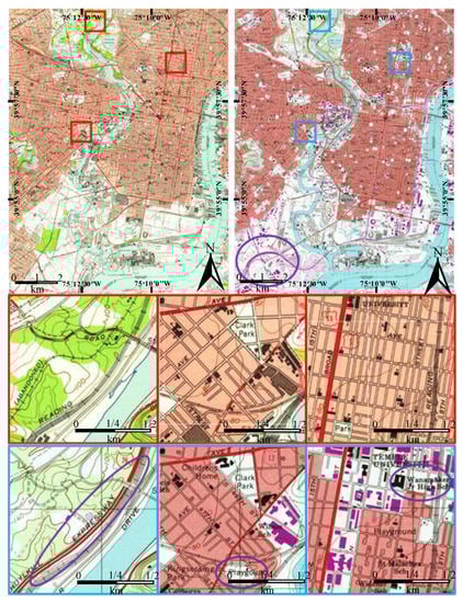
Figure 1.
United States Geological Survey (USGS) topographic maps of a Philadelphia area at 1:24,000 scale, drawn in 1949 (top left) and 1995 (top right). Second and third rows are selected small regions (red and blue boxes) showing changes after these 46 years. Purple circles indicate examples of new geographic elements, such as the expressway and high school.
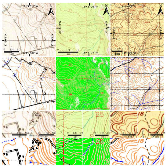
Figure 2.
Samples showing the goal of segmentation of topographic maps. From top to bottom: original topographic samples of STM from USGS dataset, corresponding segmentation results, and two zoomed-in patches illustrating each segmentation in detail.
The challenges in segmenting STM have been analyzed in detail in many previous works [7,8,9,10,11,12,13,14,15]. These studies focused on the issues of color changes caused by the long storage period of paper maps, the frequent overlapping of geographic elements, and misalignment of the scanner. It seems that these challenges are no longer problems with the achievement of recent deep learning (DL) techniques in image segmentation. There are new challenges when we attempt to apply DL techniques to STM segmentation. One is creating training data, because of not only the amount of labor but also the variety of STMs. There are too many topographic map series that are largely distinguished by expressing geographic elements, such as the samples shown in Figure 2. Even for the same publisher at different times, the drawing colors can be different, as shown in Figure 1. Therefore, it is hard to create a uniform dataset to build DL models. Another challenge is the scanning resolution of the STM. Usually, a topographic map has a size of around one square meter, which leads to constraints on the scanning resolution of such a large map because of the memory cost. This is why some geographic elements, especially linear ones, have very thin shapes (two to four pixels wide). With such a small width, the large proportion of false colors and mixed colors can mislead the training models (for example, two of four pixels located on the boundary, which means half of them are affected by color aliasing). Even with limited scanning resolution, an STM always has tens or even hundreds of millions of pixels. It is also a challenge to directly process such a large image by DL algorithms or any other complex model.
Some terminology is explained here to avoid confusion. Feature denotes the characteristics used to distinguish different pixels/superpixels, including handcrafted or learned ones. STMs consist of linear and area elements. Linear elements are close/not-close curves, which include point symbols and lines, such as text, contour lines, and roads. Area elements are the remaining geographic elements that are lighter in color than linear elements, such as vegetation and background. Superpixels denote a homogeneous image region that aligns well with geographic element boundaries.
1.2. Related Work
The goal of STM segmentation is to separate different geographic elements into different image layers. Fortunately, in most topographic maps, each type of geographic element is typically assigned a unique predefined color. Therefore, in many previous works, the color (or grayscale value) of each pixel is considered the most representative feature to distinguish different geographic elements in an STM. Mello et al. [16] used thresholding and denoising to extract text from grayscale maps. This method is only useful for high-quality map images, rarely applicable for typical STMs. Techniques such as the methods proposed by Dhar et al. [17] and Cordeiro et al. [18] implement segmentation processing in color spaces. Because the color information is the only feature used in segmentation, this type of method also has inaccuracy problems. Ostafin et al. [19] jointly applied thresholding on the color space and morphological operations on the image to segment forest from STM. It is efficient and easy to implement but also lacks expansibility to other geographic elements. The histogram-based approach [20,21,22], another segmentation method that focuses on color distribution, can rarely achieve satisfactory performance with poor-quality STMs.
As color information is not sufficient to accurately segment poor-quality STMs, many works consider the plane information and local neighborhood relationship as additional features. Khotanzad et al. [13] used a linear fitting method to determine the distribution of true color and aliasing color from training patches. The authors used the fitted model to decrease false segmentation. Leyk et al. [12] used a homogeneity-based seeded region-growing method to utilize the color homogeneity and local neighborhood relationship, which can improve the segmenting accuracy.
The two methods above take pixels as operating units and calculate the local neighborhood relationship in a fixed-size region, which hampers the achievement of satisfactory results on poor-quality STMs. Liu et al. [8] used fuzzy clustering to find seeds in the contour line layer and applied a specific region-growing approach to extract the contour line layer from the STM. This method overcomes the data imbalance issue of the clustering method and the growing order problem of the region-growing method, as the extracted contour lines show strong consecutiveness and accuracy; however, it is designed for the contour line layer only and lacks generalizability for the extraction of other geographic elements.
In recent years, STM segmentation methods based on region information have been proposed [7,9], in which pixels are no longer the processing object. In one method [7], linear elements are extracted at the beginning and the classifying operations are applied to independent linear elements, as segmentation is equivalent to classifying these linear elements. Area elements such as vegetation or the lack thereof are not considered. In another method [9], over-segmented superpixels are generated for each given STM; then, a support vector machine (SVM) is trained based on handcrafted color and texture features extracted from manually labeled superpixels and employed to classify the remaining ones. These two methods can overcome false color and color aliasing problems by applying region-based principles. The features which they use are still artificially designed and are not suitable for all types of STMs. In addition, the over-segmentation problem of superpixels generated using the second method [9] leads to instability of the connectedness in segmentation results.
Superpixels have been widely used in many computer vision tasks [23,24,25,26]. In the standard definition, a superpixel is a homogeneous region, which means that it contains the pixels from one object. The use of superpixels has become increasingly popular in the computer vision field. As we previously noted [14], most classical superpixel-generating methods [27,28,29,30,31] generate superpixels using over-segmentation or low boundary adherence on the STM. As shown in Figure 3, the proposed Guied Superpixel Method for Topographic Map (GSM-TM) [14] has superior accuracy on boundary adherence; however, over-segmentation still exists in the area element. DL techniques, which are extremely popular in many computer vision fields, also have been applied in superpixel generation [32,33]. These methods have satisfying performance on natural images but also have expensive computational costs. In addition, some are supervised methods that require ground truth labels to train the network [32]. Suzuki [33] proposed an unsupervised method that uses convolutional neural networks (CNNs) to optimize a proposed objective function that consists of entropy-based clustering cost, spatial smoothness, and reconstruction cost. Although it has superior performance on natural image datasets, compared with classical methods such as Simple Linear Iterative Clustering (SLIC) [27], the computational cost for training a CNN model is also higher.
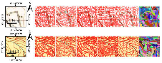
Figure 3.
Superpixel generation results. From left to right: original map, GSM-TM [14], normalized cut (NC) [28], watershed [31], SLIC [27], turbopixel [30], and graph-based segmentation [29] results.
Many superpixel-based segmentation methods use handcrafted features extracted from the superpixels as input to various classifiers [9,34,35]. Artificial features are difficult to design appropriately for all types of STM. Determining the weights of features is another challenge in segmentation. CNNs can extract deep features from images without manually assigned features and are widely used in pixel-level [36,37] and superpixel-based [38,39,40,41] segmentation tasks. Pixel-level methods such as the popular fully convolutional networks [36] achieve pixel-level prediction by upsampling from feature maps. These methods cause coarse segmentation that is not suitable for segmenting fine elements from STMs. Superpixel-based methods typically apply state-of-the-art methods that generate compact and normalized superpixels [27]. To the best of our knowledge, few methods can extract features from superpixels with great differences in shape and size, such as those generated using GSM-TM. Most existing methods use unified patches either around [41] or overlapping [40] the superpixels as input to CNNs. A regular size might contain several superpixels from various geographic elements due to their dense distribution. Therefore, typical CNNs are inappropriate for the classification of superpixels applied to STMs.
1.3. Contributions
This paper presents an STM segmentation method based on superpixels and a shallow convolutional neural network (SSCNN) to overcome the above challenges and fill the technique gaps. In this algorithm, we consider the superpixels that are generated by the proposed advanced guided watershed transform (AGWT) as the classifying objects. Then, the segmentation results are obtained using the superpixel classification results. The main contributions of this paper are as follows: (i) We present a novel STM superpixel generation AGWT method. It solves the over-segmentation issue and has a strong boundary adherent ability. (ii) We apply a randomly selected unifying method to generate training and testing datasets. There are two significant advantages to this unifying method. With unifying, the SSCNN can handle superpixels of any size and shape. In addition, an extensive training dataset can be generated based on a few manually labeled pixels. (iii) A shallow CNN (SCNN) is employed to achieve the final segmentation by classifying the unified pixel sequences. It is accurate, efficient, and practical, which enables the rapid segmentation of large STMs.
2. Materials and Methods
The SSCNN procedure is shown in Figure 4. An advanced guided watershed transform method is presented and applied to the original STM to obtain superpixels. For each superpixel, a fixed-length pixel sequence is determined using random selection. Then, these pixels are input into the SCNN to predict the classification of superpixels. After the superpixels are classified, the segmentation result is obtained.
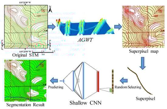
Figure 4.
Flowchart of the superpixel-based shallow convolutional neural network (SSCNN) method.
2.1. Advanced Guided Watershed Transform
We previously presented a guided superpixel generation method, GSM-TM [14], and achieved satisfying results with strong boundary adherence. The over-segmentation problems were prevented in linear elements, which significantly enhanced the continuity of linear elements; however, the over-segmentation in area elements was still not solved. We developed a novel superpixel generation method, advanced guided watershed transformation (AGWT), which overcomes the remaining over-segmentation problem in GSM-TM.
Similar to GSM-TM, the linear element is still a key clue to remove weak boundaries, but the difference is that we also apply the area elements as a clue in AGWT. The main procedures can be seen in Figure 5, including boundary detection, linear and area element (L&A) separation, guided boundary modification, and the final watershed transform.
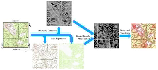
Figure 5.
Advanced guided watershed transformation (AGWT) procedure.
A boundary detection method based on color-opponent mechanisms of the visual system, proposed by Yang et al. [42], was utilized to generate a boundary image from a given STM . This method has good sensibility in color changes and therefore is very suitable for applying to STM, because topographic maps are always drawn with visually distinguished colors to represent different geographic features. This boundary detection method can achieve strong boundaries on the true edges but also has many weak boundaries on the false edges, such as in the interior of linear elements as well as area elements (as shown in Figure 6).
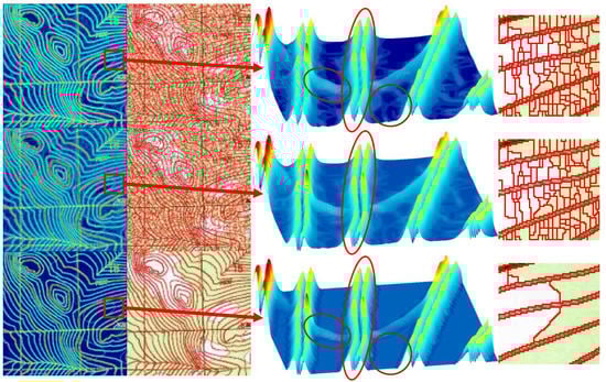
Figure 6.
Illustration of boundary modification. Top row: original unmodified boundary and corresponding watershed transformation. Middle row: modified boundary and generated superpixel of GSM-TM. Bottom row: modified boundary and generated superpixel of AGWT. From left to right: boundary map, superpixel image, 3D model of boundary in a small patch, and corresponding superpixel in this patch. Red and brown circles indicate how AGWT solves the false boundary wall issue on linear elements and area elements, respectively.
L&A separation is performed based on a compound opposite Gaussian filter (COGF) and shear transform, which was presented in our previous work [14]. The main idea of this method is to use a specially designed COGF to match the region intensity gap between linear elements and area elements. The soft edges of the COGF can perfectly counteract the drawbacks of mixed color and color aliasing. Meanwhile, shear transform helps to add the directions to make sure all parts of the linear elements in any orientation can be accurately matched. This method was verified to have excellent performance on linear extraction. To utilize it for L&A separation, we made a few changes to this method. One was that we increased the number of shear transform directions from 3 to 17, from −80° to 80° with a step of 10°. We found that this small change could largely improve the quality of the extracted linear element in both continuity and accuracy. Another change is that linear elements are not the only output of this method; area elements are also achieved. Area elements can be regarded as complementary to linear elements, which include background and all geographic features with a broad continuous region—for instance, vegetation (green areas), as shown in Figure 5. Morphology erosion is applied to the complementary linear element regions to obtain pure area element regions, which can be described by Equation (1):
where is the linear element region, is the area element region, and represents the morphology erosion operation.
The strengths of false boundaries in linear elements and area elements are significantly different. Some false boundaries in a linear element are even stronger than the true boundaries in the area element. Therefore, it is hard to find a uniform modification method that makes the boundary modification contain two independent strategies for and .
The strategy for modifying is based on its own shape. It is built on the fact that different geographic elements can intersect. Therefore, in , the true boundaries between two linear elements should only be contained in the cross regions, which means that the false boundaries appear in non-cross regions. Based on this fact, is thinned by mathematical morphology into the single-pixel skeleton to find the cross point set . Then, we set a certain range around cross points as the cross regions. Those boundaries along , but out of the cross regions, are false boundaries, which should be removed. The boundary modification in can be described by Equation (2):
where represents any pixel in and the distance is the number of pixels in the nearest path between and cross point . After modification, all those false boundary walls in will be broken with small holes, which means that there will not be any edges on those false boundaries after subsequent watershed transform (as indicated by the red circles on the 3D models in Figure 6). It should be noted that this modification strategy has a similar fundamental idea as in GSM-TM, which is to reduce the strengths of false boundaries based on their distance from the cross points, only it is simpler and more practical. This is why the modified boundaries in linear element regions seem the same for GST-TM and AGWT in Figure 6.
In , although both false and true boundaries always have relatively lower strength compared to , there is still a difference in their strength (see the 3D model in the top row of Figure 6). Therefore, we apply a thresholding method to modify the boundary map in , which can be expressed by Equation (3):
where is the threshold calculated by Otsu’s method [43], is the Hadamard product, and means to take the maximum in a and b. After this modification, the true boundaries are kept, but the false boundaries will be removed (see the brown circles on 3D models in Figure 6).
Finally, a watershed transform is applied to the modified boundary map that combines the modifications in and , to achieve the superpixel image, as shown in Figure 6. In the subsequent experiment section, the advantages of AGWT will be further analyzed.
2.2. Superpixel Unification
Intuitively, two ideas inspired classifying those superpixels that are very different in size and shape. One is similar to that in a previous study [9], which extracts the features based on artificially designed features, such as mean colors and textures, and then performs classification based on the similarity of those artificial features. Another idea is to unify those superpixels into the same size and then partition them based on the similarity of the unified units. In our method, we prefer to use the latter strategy. The unifying approach that we applied was based on the idea of random selection. We believe that random selection will keep the main features, since the color information plays a crucial role in STM image processing and recognition [7,8]. Although the texture information can help to distinguish different types of superpixels, it is not comparable with the color information. Randomly selected pixels from one superpixel are in a different order but have a similar color. The idea behind this unifying strategy is to utilize a large amount of random selection to cover the color varieties in STM. That is, while the randomly selected training data are sufficient, they can easily express the color distribution of those geographic elements. We believe that this approach maintains the most crucial information in the superpixels during unification.
Assume that there are superpixels in a given STM. All superpixels are unified to pixel sequences . Each superpixel contains pixels. means copy all pixels in times, and means randomly select pixels from . represents the ceil function. Our superpixel unification method can be described by Equation (4):
Notably, Equation (4) is used to generate only the testing dataset from the superpixels. represents a batch of labeled pixels that are unnecessarily contained in one superpixel or even one region.
There are three advantages to this unification method: (i) All superpixels can be converted into a pixel sequence of the same length, regardless of their size or shape. (ii) The most important information, color, is mostly maintained. (iii) Random selection can create flexible amounts of training data with very few labeled geographic elements. For instance, if we extract a pixel sequence from manually labeled pixels, there could be different choices. If we consider the order in the pixel sequence, the number is much higher. The imbalanced data problem is also solved because we can create large training datasets from very few labeled pixels.
2.3. Shallow Convolutional Neural Network
We utilize an SCNN in our algorithm to classify into different categories. The reason we choose CNN over the conventional neural network for classification is that there is still homogeneity among the pixels in a randomly generated pixel sequence. Although the random selection will lose the texture information in a superpixel (as discussed in Section 3.2), the similarity of color still remains. Therefore, local color information, even in pixel sequences, should be helpful in distinguishing different geographic elements. Meanwhile, compared with the fully connected neural network, CNNs have a relatively small number of parameters to train. We chose a shallow network because we found that a deeper CNN with multiple convolutional layers or multiple fully connected layers did not improve the accuracy, but it easily tended toward an undesirable state of becoming trapped at a local optimum at the beginning (see Appendix A for more experimental proof).
The SCNN that we apply in the SSCNN is illustrated in Figure 7. In this network, there is only one convolutional layer and one fully connected layer. Assume that there are Cl geographic categories in the given STM; is the length of the input pixel sequence, and the size and number of convolutional kernels are Cs and Cn, respectively. After convoluting with a stride of 1, Cn feature maps can be obtained and input into the activation function. Then, the output of the activation function is reformed into a vector and fully connected with Fc nodes. After this, Cl nodes are fully connected, and finally, the classification is performed through softmax. This SCNN is simple and easy to perform. Importantly, it is speedy for both the training and testing periods.
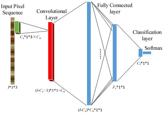
Figure 7.
Shallow CNN architecture.
In the segmenting stage, a straightforward ensemble learning strategy, multiple predictions, is employed to predict each superpixel. It means that each superpixel will randomly generate pixel sequences; thus, there will be predictions for each superpixel. The final class of the superpixel should be the most frequent one among those predictions. The idea behind this strategy is to utilize the law of large numbers against randomness, which makes the prediction more robust. It is also feasible in terms of computational cost because of the efficiency of SCNN and the relatively small number of superpixels in our algorithm.
2.4. Parameters
There are three parts in the SSCNN, which are superpixel generation, superpixel unification, and the SCNN.
In superpixel generation, the parameters are mainly in the linear element extraction procedure [14]. and in the COGF are applied to control the shape of the filter operator. In addition, a threshold is applied to distinguish linear elements and area elements, which is necessary after filtering. In our experiments, these parameters must be adjusted according to each type of STM. For most types of STM, and can be set as 1 and 3, respectively. depends on the linear element thickness and should generally be larger if the linear elements are thick and smaller if they are thin. is responsible for matching the area element; therefore, it should be given a relatively large value, such as 3. For , it depends on the color contrast between the linear elements and area elements. It ranged from −50 to −450 in our experiments. The range , which is used for determining cross regions around cross points during boundary modification, is set as 5 pixels.
For superpixel unification, i.e., random selection, we set the size of unified pixel sequences as the median size (number of pixels) of all superpixels in an STM. The unified pixel size can be less than that of 50% of the superpixels generated using AGWT. Therefore, these pixel sequences will not contain highly redundant information due to the low frequency of replication. As a result of AGWT being able to prevent over-segmentation of STMs, is usually not very small (mostly larger than 10). Therefore, it is strong enough to prevent the noise influence that occasionally arises from the inaccurate partitioning of superpixels during random selection. In the segmentation procedure, , which is the number of pixel sequences generated from each superpixel, is set as 10.
The other parameters in the SCNN shown in Figure 7 include the number and size of convolutional kernels, the number of neural nodes in the fully connected layer, and the activation function. As a result of the fact that the SCNN contains only two layers, the vanishing gradient problem in the sigmoid function is not an issue. Therefore, we applied the sigmoid function as the activation function in the SCNN. We set the size and number of the convolutional kernels as 5 and 15, respectively. The fully connected layer contains 50 neural nodes, and the node number Cl in the output layer depends on how many geographic categories are included in the given STM. These parameters were the optimal ones found during the development of our algorithm and the subsequent experiments, and they can maintain that the proposed method has a satisfactory and robust performance.
2.5. Procedures
The training dataset was generated from a group of manually labeled pixels. As in previous research [9], we manually drew some short lines on each element, which means that in each STM, for each type of geographic element, a few manual drawing lines are needed. All superpixels covered by these lines were considered true superpixels. In contrast to previous research [9], all pixels in the true superpixels were merged into a pixel set for each element . Therefore, the training pixel sequence can be repetitively created from using Equation (4). The size of can be much larger than . Therefore, a large training dataset can be generated, which guarantees sufficient training data.
We trained the SCNN using stochastic gradient descent with a batch size of 200 sequences. The momentum was initially set to 0.5 and increased to 0.95 after 2 epochs. We did not apply a weight decay strategy in updating the weights and neuron biases. We initialized the weights from a zero-mean Gaussian distribution with a standard deviation of 0.1 and neuron biases with a constant of 0 in each layer. The learning rate was 0.1 at the beginning and was divided by 10 in every 5 epochs, up to a 3-fold reduction. All SCNNs were trained for 20 epochs.
2.6. Datasets
First, we tested the SSCNN on an STM dataset that contained 15 manually labeled STMs. The size of all the STMs was from 467 × 510 pixels to 536 × 730 pixels, cut from different series of USGS and Swisstopo STMs. Because labeling is extremely time-consuming, it is difficult to create ground truth on full-size STMs. Therefore, the dataset was used to evaluate the segmentation results quantitatively. To further assess the performance of the SSCNN, we also applied it to some large or full-size STMs and visually represented the segmentation results.
3. Results
3.1. Advanced Guided Watershed Transformation
The performance of AGWT is assessed both visually and quantitatively in this section. Some popular superpixel methods, including SLIC [27], normalized cut [28], graph-based segmentation [29], turbopixel [30], and watershed [31], were analyzed while GSM-TM was used, and GSM-TM was shown to have superior results [14]. Therefore, instead of using all of the above methods, we only employed GSM-TM as the comparison method to further evaluate the performance of AGWT. Suzuki’s unsupervised CNN-based method [33] was also used as a comparison. In this method, there are three key parameters, , , and , that control the superpixel number, the smoothness, and the weight of reconstruction cost, respectively. It is worth noting that the CNN-based method requires large GPU memory during the processing. We performed the experiments with only this method on a desktop computer with NVIDIA TITAN Xp GPU (12 G memory). We considered all three parameters with our best efforts for each STM during the experiments. Figure 8 illustrates the generated superpixels of the three methods on five STMs. In addition, boundary recall (BR; the higher, the better), boundary precision (BP; the higher, the better), and under-segmentation error (UE; the lower, the better) [44] were employed to assess the results. Since the locations of edges are usually flexible during digital image processing, conventionally, a one-pixel buffer is utilized to assess boundary accuracy (BP and BR). The quantitative assessments are shown in Table 1. Meanwhile, Table 2 gives the number of superpixels generated on each STM by the three methods.
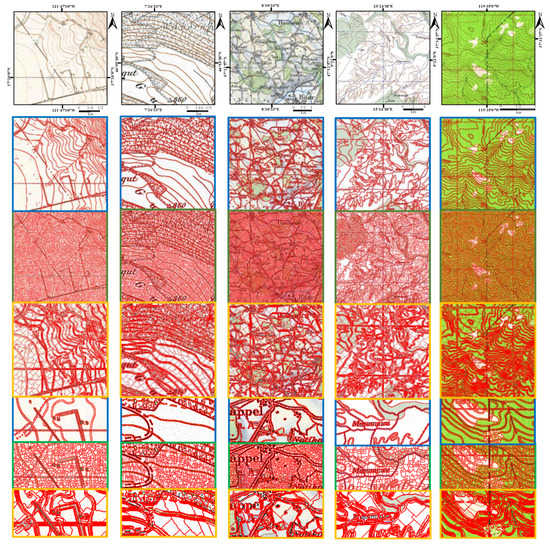
Figure 8.
The superpixel results of AGWT (blue bounding box), GSM-TM (green bounding box), and unsupervised CNN-based [33] method (orange bounding box). Each column shows the results of one sample STM. From top to bottom are the original STM, the results of AGWT, GSM-TM, CNN-based method, and the zoomed-in patches of the three methods, separately.

Table 1.
Mean (standard deviation) of boundary recall (BR), boundary precision (BP), and under-segmentation error (UE) achieved by CNN, GSM-TM, and AGWT on the STM dataset.
Table 2.
Amount of superpixels generated by GSM-TM, AGWT, and unsupervised CNN.
3.2. Shallow CNN Segmentation
As discussed in previous work [9], superpixel-based methods have been shown to perform better than pixel-based methods [12,13]. Therefore, we employed only superpixel-based methods to demonstrate the performance of the SSCNN. One method was Superpixel-based Color Topographic Map Segmentation (SCTMS) [9], which segments STMs based on superpixels and a support vector machine (SVM). SCTMS utilizes an over-segmented superpixel partition from the watershed transform and employs manually designed features on color and texture. To demonstrate the advantages of the feature extraction ability of SCNN, we used AGWT to generate superpixels. Then, we applied the SCTMS framework, including SVM strategies and features, to classify the superpixels, termed AGWT+SVM. For comparison, we used the same superpixels in the training procedure for both methods. We adopted the classic evaluation metrics (precision, recall, and F1 score [45]) to measure the segmentation quality.
Figure 9 shows a group of segmentation results on a sample STM and zoomed-in patches from the results to demonstrate the performance of SSCNN, AGWT+SVM, and SCTMS. To further illustrate the experimental results, patches of the segmentation results cut from different testing STMs are shown in Figure 10. In these results, each segmented geographic element is given a similar color to that of the original STM. The small patches are 200 × 200 pixels in Figure 9 and Figure 10. In addition to the visual results, the quantitative evaluation results are shown in Table 3.
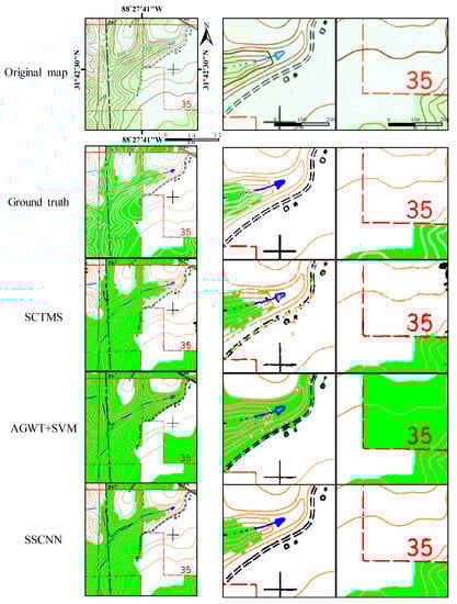
Figure 9.
Sample map and segmentation results of SCTMS, AGWT+SVM, and SSCNN. Left row shows whole map, ground truth, and segmented results. Middle and right rows are the corresponding amplified patches.
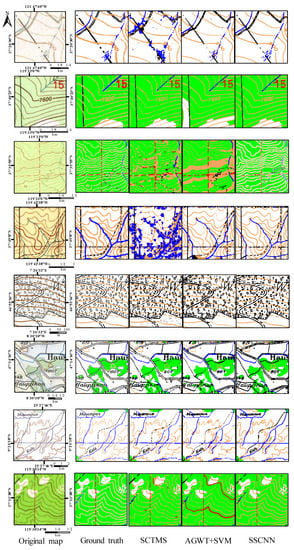
Figure 10.
Sample patches cut from map dataset and corresponding ground truth and segmentation results. From left to right: original map, manually labeled ground truth, segmented results of SCTMS, AGWT+SVM, and SSCNN, respectively.
Table 3.
Precision, recall, and F1 score for all methods on an STM dataset. Mean (standard deviation) is shown.
To further explore the practical application of SSCNN, we applied it to large and full-size STMs, the original STMs that were cut to form the previously used STM dataset. These STMs were from 2283 × 2608 to 6444 × 8035 in size. As a result of the fact that the STMs in our dataset are part of the full-size STMs, we used the already-trained network models from previous experiments to segment them directly. Due to space limitations, we illustrate only one large STM and some magnified patches in Figure 11.
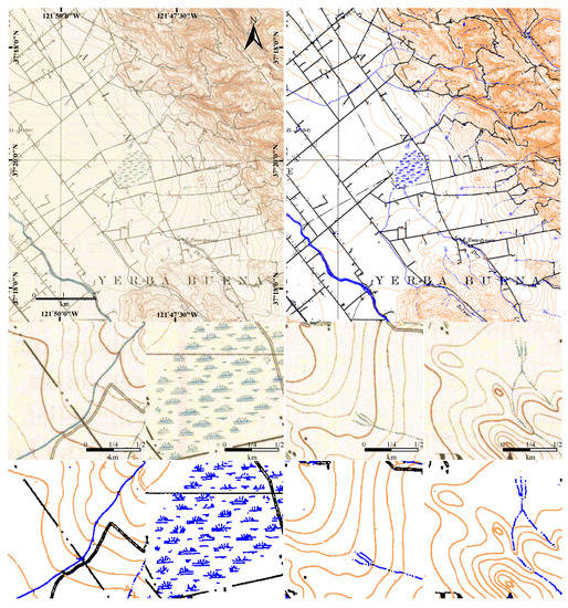
Figure 11.
SSCNN on a large map, with amplified sample patches. Top left is a large STM from USGS dataset and top right is the segmentation result. Two bottom rows are amplified cropped patches to show the results in detail.
SSCNN applies a very shallow network to accomplish the classification; therefore, it can rapidly train SCNN and classify all superpixels through the trained SCNN. Similar to GSM-TM, AGWT has computational complexity approaching , where is the number of pixels in the STM. With these two efficient components, SSCNN can rapidly segment large STMs. Here, we illustrate a 5000 × 3810 pixel STM to demonstrate the efficiency of SSCNN. The computational time was estimated for a modern desktop computer with the following specifications: 4-core Intel Core 4.2 GHz base CPU with 8 GB RAM running the Windows 10 operating system. All algorithms were coded in MATLAB or Python(see Supplementary Materials). In the training steps, it took approximately 8 s to prepare 5 × 104 pixel sequences and 19 s to train an SCNN based on these pixel sequences for 20 epochs. In the classification procedure, it took 440 s, 10 s, and 27 s to conduct AGWT, prepare testing data, and classify using SCNN, respectively. In addition to finishing the superpixel labeling for each geographic element, less than 9 min were needed to segment a 5000 × 3810 pixel STM, including all training and classification procedures.
To further demonstrate the efficiency of SSCNN, a sequence of experiments was conducted on various sizes of training datasets and STMs. We trained the SCNN using different numbers of pixel sequences, from 5 × 10³ to 5 × 10⁴. The running times for generating data and training the SCNN and the total time are shown in Figure 12.
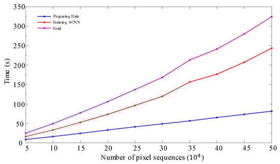
Figure 12.
Training step run time for different sizes of datasets.
Then, we cut 10 patches with the sizes from 500 × 300 to 5000 × 3000 from the previous testing STM. We applied SSCNN on those STMs with the same SCNN model instead of going through the training procedure repetitively and recorded the running time for each segmentation. Figure 13 shows the detailed running time for various sizes and the time cost tendency with STM size.
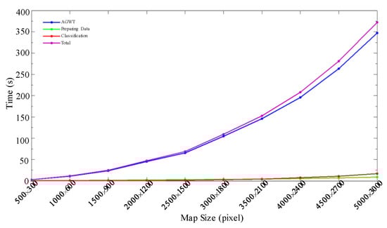
Figure 13.
Segmentation step run time for different sizes of STMs.
4. Discussion
4.1. Advanced Guided Watershed Transformation
From the results shown in Section 3.1, we can see that AGWT has superior performance compared with the other two methods. In Figure 8, the images demonstrate that AGWT can solve the over-segmentation issue in the area element, even in the heavy noise area (second column) and the shallow area caused by paper fold (third column). AGWT has a strong boundary adherent ability, as proven by the high coincidence between the superpixel boundaries and the geographic element edges.
The occurrence of less over-segmentation can also be quantitatively evaluated from Table 2, which shows that AGWT generates far fewer superpixels than GSM-TM. Although with only one-eighth to one-half of the superpixels compared to GSM-TM, the edges between different geographic elements, especially between area elements (for example, the vegetation area and the background), are well retained in AGWT, as shown in the third to fifth columns of Figure 8. The quantitative assessment in Table 1 further demonstrates the strong boundary adherent ability of AGWT. Compared to GSM-TM, AGWT has a significant increase in BP (around 0.4), with only a small reduction in BR (around 0.02), which also should contribute to the reduced over-segmentation. More importantly, with fewer superpixels, AGWT still achieves an average of 0.06 on UE, which is superior to GSM-TM. Compared with the CNN-based method, AGWT has better performance in all three metrics. This further proves that AGWT is a more qualified approach for STM than those popular methods, even DL-based approaches with high computational cost, applied for natural images. In summary, AGWT has strong boundary adherent ability (from Table 1) and less over-segmentation (from Table 2), making it suitable for superpixel generation on STM.
4.2. Segmentation
As shown in Figure 9, SSCNN can maintain linear elements with good smoothness and connectivity. Compared with the other two methods, there are fewer false classifications in the SSCNN results, such as the parallel broken black lines in the middle column and the brown lines and green areas in the right column. AGWT+SVM shows serious false segmentation in the green layer, which does not occur in SSCNN.
Figure 10 also shows this effect. For instance, the brown contour lines of SSCNN are always smoother than those of SCTMS and have better connectivity. In the classification, there are many misclassifications in AGWT+SVM and SCTMS, such as the blue layers in the first and third rows of SCTMS and the brown layers in the eighth row of AGWT+SVM and the ninth row of SCTMS. In SSCNN, the main bodies of all geographic elements are correctly segmented. This advantage should contribute to the strong feature extraction ability of SCNN. Although color noises exist in these superpixels, the potential features of geographic elements can be accurately extracted, therefore improving the segmentation accuracy. The superior performance of SSCNN can also be observed from the quantitative evaluation results shown in Table 3. SSCNN achieves precision and recall, with mean values of 0.73 and 0.76 and standard deviations of 0.17 and 0.14, respectively. These are statistically significantly higher than the results of SCTMS and AGWT+SVM (p < 0.05). For the F1 score, SSCNN achieves a mean of nearly 0.73, with a standard deviation of 0.11, which is also a statistically significant superior result (p < 0.05) compared to the other two methods. Overall, SSCNN can obtain more accurate segmentation results with stronger stability. Notably, the evaluation results in Table 3 were directly computed regarding the ground truth with no buffers. This means that even a one-pixel difference from the labeled ground truth will cause a decrease in these metrics. Therefore, an F1 score approaching 0.73 should be considered as an indication of excellent segmentation of an STM.
We believe that the superior performance of SSCNN results from two advantages. The first is the excellent superpixel partition results. AGWT can prevent over-segmentation, which guarantees segmentation results with connective geographic elements. The good boundary adherence ability enables smoothly segmented elements. It can avoid the effect of “color noises” (including color aliasing, false colors, and mixed colors) and, at the same time, keep the smoothness and connectivity of linear geographic elements. The second advantage is the strong feature extraction ability. The random selection can maintain most color information, the most crucial information in STMs, in the fixed-size pixel sequences. A shallow network can accurately abstract the input pixel sequences and classify them. SSCNN has powerful feature extraction and accurate classification ability, leading to excellent segmentation on STMs. In summary, SSCNN can achieve more accurate segmentation performance than currently existing solutions and can handle challenging, poor-quality STMs.
The main body of each geographic element is successfully segmented in the STM shown in Figure 11. In addition, details of segmentation results can be observed from the amplified sample patches. The detailed information of geographic elements is accurately segmented in most cases, such as wetlands, roads, contour lines, and rivers. The color distortion consists of background and geographic elements, which can be observed in the amplified patches, especially in the background, but did not cause much false segmentation. These results show that SSCNN can achieve excellent performance in segmentation accuracy.
In addition to accuracy, the efficiency of the training and testing procedures of the SSCNN is demonstrated in Figure 12 and Figure 13, respectively. Figure 12 shows the curves of time cost along with the increased size of training datasets. The time costs of preparing the dataset and training the SCNN are almost linear to the length of the pixel sequence. Only less than 6 min is required for the training step with 5 × 104 pixel sequences, which means less than 0.001 s per pixel sequence for training. Figure 13 demonstrates the segmenting speed, where the time cost for data preparation and classification is almost linear along with the STM size. Moreover, the increased time spent by AGWT approaches times the STM size, where N is the STM size. We can see from Figure 13 that the size difference between the smallest and largest STM is 100 times, and the time increased by approximately 150 times. Considering the STM size and time required for manual labeling [6], SSCNN can be regarded as an extremely efficient algorithm. This approach can be directly applied to full-size STMs to achieve reliable segmentation quality in a very short time. We believe that it can make a large contribution to the field of information extraction from STMs.
5. Conclusions
Motivated by applications in topographic map information extraction, our goal was to seek a practical method for map segmentation that is automated, accurate, and efficient. We designed a segmentation method, named SSCNN, with superpixel generation, unification, and classification. One particular advantage of SSCNN is that it allows superpixels with a variety of shapes and sizes to be used as input. This provides the foundation of a superpixel-generating method that can create accurate region partitions according to the geographic element distribution, without considering uniformity in shape and size. This point drives us to put forward AGWT, which creates fewer over-segmentation superpixels but has strong boundary adherence, which achieves an average of 0.06 on under-segmentation error, 0.96 on boundary recall, and 0.95 on boundary precision. In this work, we demonstrated segmentation using SSCNN and two other state-of-the-art methods. SSCNN has superior performance with an overall F1 score of 0.73 on our STM testing dataset. The visual and quantitative results show that SSCNN had superior performance. Through a discussion of the computational complexity and an illustration of the computational time, SSCNN was shown to be an efficient algorithm. One shortcoming of this paper is the small number of image datasets utilized. Unfortunately, the manual labor required to establish ground truth often becomes a bottleneck in selecting appropriately sized datasets.
Supplementary Materials
The codes are available on https://github.com/wolfman623/SSCNN.git.
Author Contributions
Conceptualization, T.L. and Q.M.; methodology, T.L. and P.X.; software, T.L. and P.X.; validation, T.L. and S.Z.; formal analysis, Q.M. and S.Z.; data curation, T.L.; writing—original draft preparation, T.L., Q.M. and P.X.; writing—review and editing, T.L., Q.M. and S.Z. All authors have read and agreed to the published version of the manuscript.
Funding
This research was supported in part by the National Natural Science Foundation of China under grant nos. 61802335, 61772396, 61973250; the Natural Science Foundation of Hebei Province of China under grant no. F2018203096.
Acknowledgments
We acknowledge the use of STM data from the USGS (https://nationalmap.gov/historical/) and Swisstopo (https://map.geo.admin.ch/) websites.
Conflicts of Interest
The authors declare no conflict of interest.
Appendix A
This section will show, instead of the SCNN we used, how a deeper CNN will affect the accuracy and stability of the segmentation performance on our STM dataset. We keep all the other procedures, including superpixel generation and superpixel unifying, as same as we described in Section 2, but we replace the SSCN with deeper CNN. We apply the same structure, where the size and number of the convolutional kernels is 5 and 15, respectively, for each convolutional layer in this experiment. After each convolutional layer, an activation function is applied before the next layer. For reducing the vanishing gradient problem, we apply the Rectified Linear Unit (ReLU) as the activation function for the deeper CNN with more than four convolutional layers.
From the results shown in Table A1 we can see that a deeper CNN with multiple convolutional layers does not significantly improve the accuracy; meanwhile, it easily tends toward an unstable model. The lower mean values and higher standard deviation from deeper CNNs have proven that an SCNN is more suitable for our approach. Especially, the high values in the standard deviation of deeper CNNs come from the failed segmentation results, which are usually caused by a failure model.
Table A1.
Mean (standard deviation) of F1 measure, precision, and recall for the segmentation results on the STM data set of different depths of CNN.
Table A1.
Mean (standard deviation) of F1 measure, precision, and recall for the segmentation results on the STM data set of different depths of CNN.
| 1 Layer | 2 Layers | 3 Layers | 4 Layers | 5 Layers | 6 Layers | 7 Layers | |
|---|---|---|---|---|---|---|---|
| F1 Measure | 0.725 (0.113) | 0.726 (0.153) | 0.704 (0.184) | 0.701 (0.173) | 0.682 (0.192) | 0.708 (0.165) | 0.660 (0.230) |
| Precision | 0.734 (0.171) | 0.760 (0.194) | 0.731 (0.231) | 0.717 (0.219) | 0.703 (0.237) | 0.736 (0.209) | 0.692 (0.268) |
| Recall | 0.758 (0.144) | 0.748 (0.168) | 0.743 (0.169) | 0.746 (0.166) | 0.725 (0.199) | 0.740 (0.176) | 0.708 (0.226) |
References
- Kienast, F. Analysis of historic landscape patterns with a Geographical Information System—A methodological outline. Landsc. Ecol. 1993, 8, 103–118. [Google Scholar] [CrossRef]
- Petit, C.C.; Lambin, E.F. Impact of data integration technique on historical land-use/land-cover change: Comparing historical maps with remote sensing data in the Belgian Ardennes. Landsc. Ecol. 2002, 17, 117–132. [Google Scholar] [CrossRef]
- Jacek, K.; Christine, E.; Mateusz, T. Forest cover changes in the northern Carpathians in the 20th century: A slow transition. J. Land Use Sci. 2007, 2, 127–146. [Google Scholar]
- Dietzel, C.; Herold, M.; Hemphill, J.J.; Clarke, K.C. Spatio-temporal dynamics in California’s Central Valley: Empirical links to urban theory. Int. J. Geogr. Inf. Sci. 2005, 19, 175–195. [Google Scholar] [CrossRef]
- Allord, G.J.; Walter, J.L.; Fishburn, K.A.; Shea, G.A. Specification for the US Geological Survey Historical Topographic Map Collection. Techniques and Methods 11–B6: US Geological Survey 2014. Available online: https://pubs.usgs.gov/tm/11b6/pdf/tm11-b6.pdf (accessed on 9 October 2019).
- Chiang, Y.Y.; Leyk, S.; Knoblock, C.A. A survey of digital map processing techniques. ACM Comput. Surv. 2014, 47, 1–44. [Google Scholar] [CrossRef]
- Liu, T.; Miao, Q.; Xu, P.; Song, J.; Quan, Y. Color topographical map segmentation algorithm based on linear element features. Multimed. Tools Appl. 2016, 75, 5417–5438. [Google Scholar] [CrossRef]
- Liu, T.; Miao, Q.; Xu, P.; Tong, Y.; Song, J.; Xia, G.; Yang, Y.; Zhai, X. A contour-line color layer separation algorithm based on fuzzy clustering and region growing. Comput. Geosci. 2016, 88, 41–53. [Google Scholar] [CrossRef]
- Liu, T.; Miao, Q.; Tian, K.; Song, J.; Yang, Y.; Qi, Y. SCTMS: Superpixel based color topographic map segmentation method. J. Vis. Commun. Image R 2016, 35, 78–90. [Google Scholar] [CrossRef]
- Miao, Q.; Xu, P.; Liu, T.; Yang, Y.; Zhang, J.; Li, W. Linear feature separation from topographic maps using energy density and the shear transform. IEEE Trans. Image Process. 2013, 22, 1548–1558. [Google Scholar] [CrossRef]
- Miao, Q.; Xu, P.; Liu, T.; Song, J.; Chen, X. A novel fast image segmentation algorithm for large topographic maps. Neurocomputing 2015, 168, 808–822. [Google Scholar] [CrossRef]
- Leyk, S.; Boesch, R. Colors of the past: Color image segmentation in historical topographic maps based on homogeneity. Geoinformatica 2010, 14, 1–21. [Google Scholar] [CrossRef]
- Khotanzad, A.; Zink, E. Contour line and geographic feature extraction from USGS color topographical paper maps. IEEE Trans. Pattern Anal. 2003, 25, 18–31. [Google Scholar] [CrossRef]
- Miao, Q.; Liu, T.; Song, J.; Gong, M.; Yang, Y. Guided superpixel method for topographic map processing. IEEE Trans. Geosci. Remote Sens. 2016, 54, 6265–6279. [Google Scholar] [CrossRef]
- Miao, Q.; Xu, P.; Li, X.; Song, J.; Li, W.; Yang, Y. The recognition of the point symbols in the scanned topographic maps. IEEE Trans. Image Process. 2017, 26, 2751–2766. [Google Scholar] [CrossRef] [PubMed]
- Mello, C.A.B.; Costa, D.C.; Dos Santos, T.J. Automatic image segmentation of old topographic maps and floor plans. In Proceedings of the IEEE International Conference on Systems, Man, and Cybernetics, Seoul, Korea, 14 October 2012; pp. 132–137. [Google Scholar]
- Dhar, D.B.; Chanda, B. Extraction and recognition of geographical features from paper maps. Doc. Anal. Recognit. 2006, 8, 232–245. [Google Scholar] [CrossRef]
- Cordeiro, A.; Pina, P. Colour map object separation. In Proceedings of the ISPRS Mid-Term Symposium, Enschede, The Netherlands, 8–11 May 2006; pp. 243–247. [Google Scholar]
- Ostafin, K.; Iwanowski, M.; Kozak, J.; Cacko, A.; Gimmi, U.; Kaim, D.; Psomas, A.; Ginzler, C.; Ostapowicz, K. Forest cover mask from historical topographic maps based on image processing. Geosci. Data J. 2017, 1, 29–39. [Google Scholar] [CrossRef]
- Zheng, H. Research and implementation of automatic color segmentation algorithm for scanned color maps. J. Comput. Aided Des. Comput. Graph. 2003, 15, 29–33. [Google Scholar]
- Salvatore, S.; Guitton, P. Contour line recognition from scanned topographic maps. In Proceedings of the WSCG, Plzen, Czech Replublic, 2–4 February 2003; pp. 419–426. [Google Scholar]
- Xin, D.; Zhou, X.; Zheng, H. Contour line extraction from paper-based topographic maps. J. Inf. Comput. Sci. 2006, 1, 275–283. [Google Scholar]
- Lu, Z.; Fu, Z.; Xiang, T.; Han, P.; Wang, L.; Gao, X. Learning from weak and noisy labels for semantic segmentation. IEEE Trans. Pattern Anal. 2017, 39, 486–500. [Google Scholar] [CrossRef]
- Li, K.; Zhu, Y.; Yang, J.; Jiang, J. Video super-resolution using an adaptive superpixel-guided auto-regressive model. Pattern Recognit. 2016, 51, 59–71. [Google Scholar] [CrossRef]
- Yang, F.; Lu, H.; Yang, M.H. Robust superpixel tracking. IEEE Trans. Image Process. 2014, 23, 1639–1651. [Google Scholar] [CrossRef] [PubMed]
- Liu, Z.; Zhang, X.; Luo, S.; Meur, O.L. Superpixel-Based Spatiotemporal Saliency Detection. IEEE Trans. Circ. Syst. Vid 2014, 24, 1522–1540. [Google Scholar] [CrossRef]
- Achanta, R.; Shaji, A.; Smith, K.; Lucchi, A.; Fua, P.; Süsstrunk, S. SLIC superpixels compared to state-of-the-art superpixel methods. IEEE Trans. Pattern Anal. 2012, 34, 2274–2282. [Google Scholar] [CrossRef]
- Shi, J.; Malik, J. Normalized cuts and image segmentation. IEEE Trans. Pattern Anal. 2020, 22, 888–905. [Google Scholar] [CrossRef]
- Felzenszwalb, P.F.; Huttenlocher, D.P. Efficient graph-based image segmentation. Int. J. Comput. Vis. 2004, 59, 167–181. [Google Scholar] [CrossRef]
- Levinshtein, A.; Stere, A.; Kutulakos, K.N.; Fleet, D.J.; Dickinson, S.J.; Siddiqi, K. Turbopixels: Fast superpixels using geometric flows. IEEE Trans. Pattern Anal. 2009, 31, 2290–2297. [Google Scholar] [CrossRef] [PubMed]
- Vincent, L.; Soille, P. Watersheds in digital spaces: An efficient algorithm based on immersion simulations. IEEE Trans. Pattern Anal. 1991, 13, 583–598. [Google Scholar] [CrossRef]
- Varun, J.; Sun, D.; Liu, M.; Yang, M.H.; Kautz, J. Superpixel sampling networks. In Proceedings of the European Conference on Computer Vision, Munich, Germany, 8–14 September 2018; pp. 352–368. [Google Scholar]
- Suzuki, T. Superpixel Segmentation Via Convolutional Neural Networks with Regularized Information Maximization. In Proceedings of the IEEE International Conference on Acoustics, Speech and Signal Processing, Barcelona, Spain, 4–8 May 2020; pp. 2573–2577. [Google Scholar]
- Csillik, O. Fast segmentation and classification of very high resolution remote sensing data using slic superpixels. Remote Sens. 2017, 9, 243. [Google Scholar] [CrossRef]
- Giordano, D.; Murabito, F.; Palazzo, S.; Spampinato, C. Superpixel-based video object segmentation using perceptual organization and location prior. In Proceedings of the IEEE Conference on Computer Vision and Pattern Recognition, Boston, MA, USA, 7–12 June 2015; pp. 4814–4822. [Google Scholar]
- Long, J.; Shelhamer, E.; Darrell, T. Fully convolutional networks for semantic segmentation. IEEE Trans. Pattern Anal. 2017, 39, 640–651. [Google Scholar] [CrossRef]
- Badrinarayanan, V.; Kendall, A.; Cipolla, R. SegNet: A deep convolutional encoder-decoder architecture for scene segmentation. IEEE Trans. Pattern Anal. 2017, 39, 2481–2495. [Google Scholar] [CrossRef]
- Gonzalo-Martin, C.; Garcia-Pedrero, A.; Lillo-Saavedra, M.; Menasalvas, E. Deep learning for superpixel-based classification of remote sensing images. In Proceedings of the GEOBIA, Enschede, The Netherlands, 14–16 September 2016. [Google Scholar]
- Gadde, R.; Jampani, V.; Kiefel, M.; Kappler, D.; Gehler, P.V. Superpixel convolutional networks using bilateral inceptions. In Proceedings of the European Conference on Computer Vision, Amsterdam, The Netherlands, 8 October 2016; pp. 597–613. [Google Scholar]
- Sakurada, K.; Okatani, T. Change detection from a street image pair using CNN features and superpixel segmentation. In Proceedings of the BMCV, Swansea, UK, 7–10 September 2015; Volume 61, pp. 1–12. [Google Scholar]
- Liu, F.; Lin, G.; Shen, C. CRF learning with CNN features for image segmentation. Pattern Recognit. 2015, 48, 2983–2992. [Google Scholar] [CrossRef]
- Yang, K.; Gao, S.; Li, C.; Li, Y. Efficient color boundary detection with color-opponent mechanisms. In Proceedings of the IEEE Conference on Computer Vision and Pattern Recognition, Portland, OR, USA, 23–28 June 2013; pp. 2810–2817. [Google Scholar]
- Otsu, N.A. Threshold selection method from gray-level histograms. IEEE Trans. Syst Man Cybern. 1979, 9, 62–66. [Google Scholar] [CrossRef]
- Wang, M.; Liu, X.; Gao, Y.; Ma, X.; Soomro, N.Q. Superpixel segmentation: A benchmark. Signal. Process. Image 2017, 56, 28–39. [Google Scholar] [CrossRef]
- Martin, D.R.; Fowlkes, C.C.; Malik, J. Learning to detect natural image boundaries using local brightness, color, and texture cues. IEEE Trans. Pattern Anal. 2004, 26, 530–549. [Google Scholar] [CrossRef] [PubMed]


Publisher’s Note: MDPI stays neutral with regard to jurisdictional claims in published maps and institutional affiliations. |
© 2020 by the authors. Licensee MDPI, Basel, Switzerland. This article is an open access article distributed under the terms and conditions of the Creative Commons Attribution (CC BY) license (http://creativecommons.org/licenses/by/4.0/).