Depth-Wise Separable Convolution Neural Network with Residual Connection for Hyperspectral Image Classification

Abstract

The neural network-based hyperspectral images (HSI) classification model has a deep structure, which leads to the increase of training parameters, long training time, and excessive computational cost. The deepened network models are likely to cause the problem of gradient disappearance, which limits further improvement for its classification accuracy. To this end, a residual unit with fewer training parameters were constructed by combining the residual connection with the depth-wise separable convolution. With the increased depth of the network, the number of output channels of each residual unit increases linearly with a small amplitude. The deepened network can continuously extract the spectral and spatial features while building a cone network structure by stacking the residual units. At the end of executing the model, a 1 × 1 convolution layer combined with a global average pooling layer can be used to replace the traditional fully connected layer to complete the classification with reduced parameters needed in the network. Experiments were conducted on three benchmark HSI datasets: Indian Pines, Pavia University, and Kennedy Space Center. The overall classification accuracy was 98.85%, 99.58%, and 99.96% respectively. Compared with other classification methods, the proposed network model guarantees a higher classification accuracy while spending less time on training and testing sample sites.

1. Introduction

The neural network-based hyperspectral images (HSI), an emerging remote sensing technology, can simultaneously detect two-dimensional geometric spatial information and one-dimensional continuous spectral information of the target object. This allows HSI the ability of "image-spectrum merging" that is the abstract feature combined image space with spectrum domain. Geometric space information reflects the size, shape and other external features of the target object. Spectral information reflects the physical structure and chemical composition of the ground object. Together, HSI extracts comprehensive characteristics of studied objects. With this, hyperspectral remote sensing is now widely used in the analysis of the composition of planets [1], marine plant detection [2], shallow river bathymetry, and turbidity estimation [3].

An important consideration for the application of hyperspectral remote sensing technology is how to build a more accurate and effective classification method. Traditional methods such as support vector machine (SVM) [4,5], 3D wavelet transform [6], and Gaussian mixture [7] usually use band selection and feature extraction to reduce the dimension of the original image and project the image into the low-level feature space. These methods often change how the original image bands are correlated, losing part of the spectral information, or failing to extract abstract features of the HSI. Needless to say, these shortcomings affect the accuracy of classified images.

For the past few years, with the application and development of deep learning technology, the convolutional neural network (CNN) has been widely used in image classification [8,9,10], speech recognition [11], target detection [12], and image semantic segmentation [13]. CNN shows powerful capabilities in extracting features on images for aforementioned fields. In order to effectively obtain spatial and spectral features of HSI and achieve more accurate classification, more and more researchers have begun to use CNN to replace traditional classification methods. Hu et al. [14] applied a convolutional neural network to the classification of HSI for the first time. They constructed a 1D-CNN that was composed of one convolution and two fully connected layers. However, the model only used spectral information to do the classification. Without considering the spatial information of HSI, their classification accuracy was slightly lower than that of conventional approaches.

Subsequently, Makantasis et al. [15] used a random principal component analysis (R-PCA) to reduce the number of spectral channels of the input image, followed by using a two-layer convolution model to encode the spectral and spatial information of the pixels, and finally completing the classification with the application of a multi-layer perceptron (MLP). They were able to achieve a high classification accuracy. However, it should be noted that using PCA to reduce the dimension would break the spectral continuity and lose some spectral information. To this end, Zhang et al. [16] expanded the training samples of the original HSI data using data augmentation and proposed a multi-channel CNN that used a one-dimensional convolution to extract the spectral characteristics of each pixel and a two-dimensional convolution to extract the neighborhood spatial features of the target pixel. The two convolution models were combined to realize classification. Yu et al. [17] also used a data augmentation method with a 1 × 1 small convolution that was pooled to extract features for effective classification. However, the way of data expansion was relatively tedious while the increase of training data undoubtedly lengthened the training time. Therefore, using the above methods for solving overfitting problems or to improve classification accuracy is not likely an optional method.

In order to fully extract the spatial-spectral information of HSI and achieve effective and accurate classification in the case of limited training samples, many of classifications using the neural network-based model tend to have deeper or wider complex hierarchical structures. Lee et al. [18] proposed a deep context CNN (DC-CNN) model based on the Inception module [19]. The DC-CNN model used convolution kernels of different sizes to combine the extracted space spectrum information in the first layer. It then used a two-layer residual structure to further extract space spectrum features. He et al. [20] constructed an M3D-DCNN model using a 3D convolution kernel that was characterized by two large-scale convolutions and one convolution layer. Moreover, Zhong et al. [21] constructed a spatial-spectral residual network (SSRN) that included spectral feature extraction block and spatial feature extraction block using 3D kernels. Wang et al. [22] used convolution kernels of 1 × 1 and 3 × 3 to extract spectral and spatial features through density connection for effective classification. Gao et al. [23] proposed the feature multiplexing module (SC-FR) that was composed of two cross-layer connected 1 × 1 small convolution kernels. The cross-layer combination increased the depth of the model and strengthened the flow and utilization of feature information to achieve an accurate classification. Paoletti et al. [24] constructed a deep residual network (pResNet) by stacking pyramidal bottleneck residual units [25] to achieve a high classification accuracy. Although the above-mentioned uses of 3D convolution or deeper CNN networks achieved good classification results to some extent, the deep layer means that the network model has more parameters, which not only increases the computational overhead, but also requires higher computer hardware equipment.

In view of the shortcomings of existing research, this work designs a lightweight deep network classification model based on learned experiences in literature [24,25]. Our model improves the pyramid residual unit [25] and replaces the standard convolution in the residual unit with a depth-wise separable convolution [26]. This model greatly reduces the number of model parameters and the computational cost. By stacking the improved pyramidal residual units, the multiplexing of low-level feature information is strengthened. In the meantime, the gradients disappearance and overfitting phenomena of deep network are alleviated. Moreover, the spatial-spectral information of HSI is used to effectively improve classification accuracy. All convolutional layers in the model, except for the residual unit, use 1 × 1 small convolutions, and the global average pooling layer is used at the end of the model to replace the fully connected layer, thereby further reducing the training parameters and accelerating the speed of classification.

2. Model Design

2.1. Depth-Wise Separable Convolution

Depth-wise separable convolution can be decomposed into depth-wise convolution and 1 × 1 convolution (also known as point-by-point convolution). Among them, depth-wise convolution is a separate convolution operation on each channel of the input image. The convolution operation is used to extract spatial features on each dimension; point-by-point convolution is a 1 × 1 standard convolution operation on the output feature map. The convolution is used to merge the feature map across channels.

As shown in Figure 1, in which the size of the input image is D_f × D_f × M, where D_f is the height and width of the input image, M is the number of channels of the map, it is assumed that the convolution kernel size is k × k in the process of depth-wise convolution, and the size of output feature map obtained by convolution is D_g × D_g × M (D_g is the height and width of the output image), which is consistent with the number of input image channels. It is used as the input of the next convolution. For the point-by-point convolution, the size of the convolution kernels is 1 × 1, the number of channels on each convolution kernels must be the same as the number of input feature map channels. Let the number of the convolution kernels be N, then the output feature map would become D_g × D_g × N after convolution.

For the input feature maps H whose size is D_f × D_f, the convolution kernel K of size is k × k. The number of input channels and the number of output channels are M and N, respectively. The size of the output feature maps G is D_g × D_g. A standard convolution operation can be defined as follows:

$$G_j = {\displaystyle \sum }_{i = 1}^M{H}_i·K_i^j+b_j, j = 1, 2, \dots , N,$$

(1)

where H_i is the ith map in H, G_i is the ith map in G, and $K_i^j$ is the ith slice in the jth kernel. b_j is the bias of output map G_i. Furthermore, the notation · stands for convolution operator. Let the total numbers of trainable parameters in convolution be P₁ (without considering bias parameters) and the number of floating-point calculations be F₁ in a standard convolution process. They can be calculated as shown in Equations (2) and (3) below:

$$P_1 = k\times k\times M\times N,$$

(2)

$$F_1 = k\times k\times M\times N\times D_g\times D_g.$$

(3)

From Equation (2), the number of parameters depend on kernel size, the number of input channels M and the number of output channels N. Equation (3) shows that the number of floating-point operations is dependent on parameter P₁ and the output feature map size D_g × D_g.

In depth-wise convolution, as shown in Figure 1, each kernel has only one piece, which is to convolute each input channel maps, and this process can be defined as:

$$G_j = H_i·K_j+b_j, i,j = 1, 2, \dots , M.$$

(4)

Here, K_j is jth depth-wise convolutional kernel. However, depth-wise convolution only filters input channels, it does not combine them to create new features. Therefore, an additional layer that is 1 × 1 standard convolution is needed in order to generate these new features [10]. For a process of depth-wise separable convolution, the parameter P₂ and the floating-point calculation F₂ are the sum of the depth-wise and 1 × 1 pointwise convolutions. Hence, P₂ and F₂ can be calculated as shown in Equations (5) and (6), respectively:

$$P_2 = k\times k\times M+M\times N,$$

(5)

$$F_2 = k\times k\times D_g\times D_g\times M+D_g\times D_g\times M\times N.$$

(6)

The ratio of Equations (5) and (2) and the ratio of Equations (6) and (3) are shown in Equations (7) and (8):

$$\frac{P_2}{P_1} = \frac{1}{N}+\frac{1}{k^2},$$

(7)

$$\frac{F_2}{F_1} = \frac{1}{N}+\frac{1}{k^2},$$

(8)

It can be clearly seen that the parameters and calculations of the depth-wise separable convolution are only $\frac{1}{N}+\frac{1}{k^2}$ times of the standard convolution. This greatly reduces the parameter and computing cost in the model.

2.2. Residual Unit

A deeper neural network tends to easily hamper convergence from the beginning. In addition, it faces a problem of network degradation [27]. To alleviate this, several studies built HSI classification models ([18,21]) through residual connection and attempted to solve the problem of deep network gradient dispersion by stacking residual modules to achieve better classification results. The basic residual unit is shown in Figure 2, where ${{\rm X}}_i$ and ${{\rm X}}_{i+1}$ are input and output of i-th residual unit. F represents a residual function. H is the way of shortcut connection: If the identity mapping [27] is used, then H (${{\rm X}}_i$) = ${{\rm X}}_i$. With these notations, the basic residual unit can be expressed as follows:

$${{\rm X}}_{i+1} = ℱ\left({{\rm X}}_i,W_i\right)+{{\rm X}}_i.$$

(9)

With the shortcut, the skipped connections increase the depth of the network, but they do not add additional parameters. Furthermore, this structure promotes the training efficiency and solves the problem of network degradation effectively [25].

Although some models constructed by the above unit have achieved good results in HSI classification, it is not the optimum. To further improve on existing models, our study introduces a pyramid residual unit [25] to promote the classification efficiency. There are two underlying ideas that guide us to do so. First, the pyramid residual unit is a modification of the basic residual unit that shows significant generalization ability [25], which will be very beneficial for the classification of hyperspectral images with unbalanced sample distribution. Second, the pyramid residual unit was the simple way to linearly increase the number of feature map channels in small steps. That greatly reduced the training parameters and computational cost of the model. Pyramid residual unit is shown in Figure 3, and unlike a basic residual unit, the last rectified linear unit (ReLU) [28] was deleted, and batch normalization (BN) [29] was required before the first convolution operation in pyramid residual unit. Specifically, the order of execution of the layers can be described as follows: BN→Conv→BN→ReLU→Conv→BN. When the number of channels after the output residual function was not the same as that of the input, the skipped connections of zero-padded [25] were performed by the element-wise addition. In addition, the original standard convolution in the unit was changed to the depth-wise separable convolution to reduce the model parameters. In short, the core parts of the network model proposed in this paper were all made of this type of unit. As the network went deeper gradually, the parameters did not increase significantly, so that a lightweight residual classification model was constructed. The specific network structure is introduced in detail in Section 2.3.

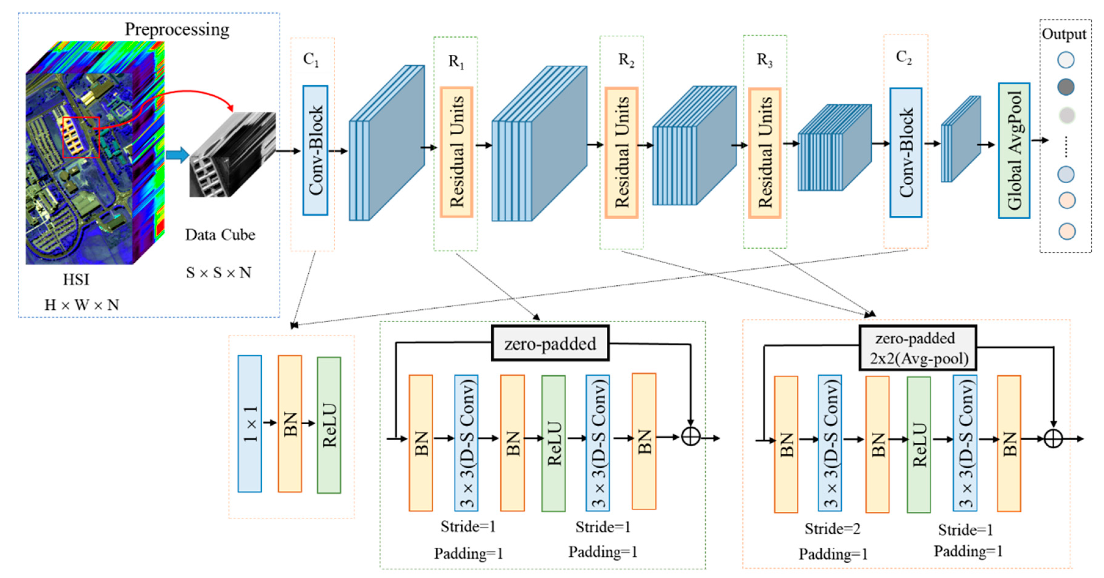
2.3. Proposed Model for HSI Classification

Here, a deep neural network model was constructed, as shown in Figure 4. In general, the model first reduced the dimension of input HSI data cube through 1 × 1 convolution, which extracted abundant spectral information. Then, the three residual units, R₁, R₂, and R₃, were adopted to extract ceaselessly both spatial contextual features and spectral features of data cube. Finally, the combination of 1 × 1 convolution and global average pooling (GAP) layer instead of the fully connected layer fused extracted abstract features to complete the final classification. The codes of this work will be available at https://github.com/pangpd/DS-pResNet-HSI for the sake of reproducibility.

Furthermore, as seen in

Table 1. The detailed configuration of the proposed network.

Layer	Output Size	Kernel Size	Stride	Padding
Input	11 × 11 × 200
C1	11 × 11 × 38	1 × 1	1	0
R1	11 × 11 × 54	3 × 3(DS-Conv)	1	1
	11 × 11 × 54	3 × 3(DS-Conv)	1	1
R2	6 × 6 × 70	3 × 3(DS-Conv)	2	1
	6 × 6 × 70	3 × 3(DS-Conv)	1	1
R3	3 × 3 × 86	3 × 3(DS-Conv)	2	1
	3 × 3 × 86	3 × 3(DS-Conv)	1	1
C2	3 × 3 × 16	1 × 1	1	0
GAP	1 × 16

, the more detailed per layer of network configuration that takes Indian Pines data set (present in

Table 2. The detailed information of three hyperspectral datasets.

	IP	PU	KSC
Type of Sensor	AVIRIS	ROSIS	AVIRIS
Spatial Size	145 × 145	610 × 340	512 × 614
Spectral Range	0.4–2.5 µm	0.43–0.86 µm	0.4–2.5 µm
Spatial Resolution	20 m	1.3 m	18 m
Bands	200	103	176
Num. of Classes	16	9	13

) as an example is listed. First, the processed 3D HSI data of which we have the shape of 11 × 11 × 200 (200 is the number of bands) was fed to the network. In the first layer C₁, 38 1 × 1 kernels reconstruct channel features of the original input data and retain the spatial information. Then, the R₁ block consisted by two 3 × 3 kernels with stride = 1 were adopted so as to remain spatial edge information. Following the R₁ block, the first layer of R₂ was the 3 × 3 filter with stride = 2 for conducting a down sampling operation, and 3 × 3 kernel in the second layer uses with step size of 1 to generate 6 × 6 × 70 feature tensors. Then, similar to the R₂ block, R₃ continues to perform the down sampling operation and produce a 3 × 3 × 86 feature cube that has a smaller space size. Finally, the C₂ in the last convolutional layer of model, which includes 16 3 × 3 kernels for compressing discriminative feature maps, post generated features to GAP layer, and then transform the shape of space into a one-dimensional vector of 1 × 16. Next, we will combine the characteristics of HSI to expound and analyze the reasons that the network was so designed.

2.4. Detailed Design of the Model

HSI have the continuity attribute that the data of each band was relatively scattered. In order to speed up convergence and reduce the training time of the model, the input data cube firstly carried out zero-mean standardization before inputting the network. The standardized calculation was defined as in Equation (10):

$${{\rm X}}_{i,j }^n = \frac{{{\rm X}}_{i,j }^n- {\overline{{\rm X}}}^n}{{\sigma }^n} \left(1\le i\le W, 1\le j\le H, 1\le n\le N\right),$$

(10)

where ${{\rm X}}_{i,j }^n$ represents the pixel value of i-th row and j-th column in the n-th band of HSI, ${\overline{{\rm X}}}^n$ is the mean value of pixels in the n-th band, ${\sigma }^n$ indicates the standard deviation of pixels in n-th band; W, H, and N denote the width, height and total number of bands of input HSI, respectively.

In order to utilize the spectral and spatial information of HSI simultaneously, the original HSI was preprocessed into a neighborhood pixel block of spatial size S × S × N as the input of the model, where S × S represents the size of the neighborhood space centered on a certain pixel and N represents the number of bands of HSI. Considering that the input HSI data cube had numerous spectral dimensions, it was easy to cause Hughes phenomenon [30]. In other words, the imbalance between high-dimensional spectral bands and a limited number of training samples tends to overfit. Therefore, as seen in the first layer of the model, the 1 × 1 bottleneck layer was used to reduce the number of original channels, so that multiple channels could be recombined without changing the size of the space. In this manner, cross channel information integration could be realized, and nonlinear characteristics could be increased (ReLU activation function after convolution was used). On the whole, the 1 × 1 convolution not only retained the original spatial information of HSI data cube, but it also reduced the spectral channel of input data and effectively extracted the spectral features of spatial blocks.

As seen in Figure 4, R₁, R₂ and R₃ were three pyramidal residual unit modules, and each module used two 3 × 3 depth-wise separable convolutions to extract corresponding features. First, the convolution operation of stride = 1 and padding = 1 was adopted in R₁, so that the input and output feature maps had the same size, and the edge space information of the feature map was retained. Then, R₂ and R₃ were the same down-sampling units, the convolution stride of the first and second layers were 2 and 1, respectively. They were used to extract the more abstract spatial-spectral information. It should be pointed out that we adopted the skipped connection of zero-padded [25] in R₁, but zero-padded with 2 × 2 average pooling was used in R₂ and R₃. The advantage of this connection was that there were no additional parameters. At the same time, normal addition operation was ensured.

In the previous convolution process, when the size of the output feature map was the same as the input or reduced to a half of the original, the number of channels of the output feature maps would be twice the original; this method undoubtedly increased the number of parameters and computation load. However, the pyramid residual unit introduced in this paper was a way to linearly increase the number of feature map channels in small steps. That greatly reduced the number of parameters and computational complexity as compared to some of the other existing methods. The calculation method of the number of output channels for each residual unit is as shown in Equation (11):

$$D_i = \{\begin{array}{c}C ; i = 1\\ \lfloor D_{i-1}+\frac{\alpha }{R}\rfloor ; i>1\end{array},$$

(11)

where D_i is the number of output channels of i-th residual unit, C is the number of initial channels feeding the first unit. That is, the number of output channels after the first layer 1 × 1 convolution, R is the total number of all residual units, and α is an integer greater than zero.

In order to avoid the information redundancy of the full connection layer, at the end of the model, 1 × 1 convolution and global average pooling layer were combined instead of using the full connection layer to fuse the features extracted from the previous layer. This approach further reduced the number of model parameters, alleviated the overfitting, and made the network to have faster convergence rate [31]. What needs to be mentioned is that the number of 1 × 1 convolution kernels should be the same as the species number of current HSI data set, so to ensure that 1 × N (N is the species number of current HSI data set) feature vector could be output from the global average pooling layer, and the final classification would be completed.

3. Experimental Setup and Parameter Discussion

3.1. Datasets Description

In order to measure the classification effect of the proposed model, three benchmark HSI data sets, Indian Pines (IP), Pavia University (PU), and Kennedy Space Center (KSC), were selected for experimental research. These data sets were available from the Grupo de Inteligencia Computacional (GIC) website (http://www.ehu.eus/ccwintco/index.php/Hyperspectral_Remote_Sensing_Scenes). The three data sets were captured at the pine testing ground in northwest Indiana, the University of Pavia in northern Italy, and Florida in the US. The details of the data sets are shown in Table 2.

3.2. Experimental Setup

The model designed in this paper was implemented by Python version 3.6.5 and the deep learning framework of PyTorch version 1.0.0 (available from https://pytorch.org). The computer hardware was Intel (R) Xeon (R) E5-2697 [email protected] CPU, the memory size was 32 GB, and the NVIDIA Tesla K20m GPU. We set the batch size of Indian Pines, Pavia University and Kennedy Space Center dataset to 64, 128, and 32, respectively. The value of α was fixed to be 48, and the learning rate was set to 0.01 uniformly. Stochastic gradient descent (SGD) optimizer was used to optimize the training parameters, and each experiment was performed 200 epochs. Besides that, all convolution layers were initialized with MSRA method [32] before training.

The experiments in this section are organized as follows. The influence of space size, initial convolution kernel number, and residual unit number on the classification accuracy were analyzed. The overall classification accuracy (OA), average classification accuracy (AA), and Kappa coefficient (K) were used as the measurement indexes of the experimental results. In order to ensure the accuracy of the experiment, each group of experiments were carried out 10 times, and the average values and standard deviation of the results of each 10-time experiment were taken as the final experimental results. To rule out variability due to random factors (training and testing sample order) in the experiment, we selected 10 different random seeds for every experiment.

In the three datasets, we randomly selected 200 samples per class object as the training set. For the Indian Pines and Kennedy Space Center datasets, however, the numbers of individual objects were less than 200, respectively. For example, the 1, 7, 9, and 16 class objects in the Indian Pines data set did make the overall sample distribution uneven. For this problem, the objects of less than 200 were randomly selected to be around 80% of the samples to be used as training set. The remaining data was used for the testing. In addition, 75% of the training samples were randomly selected for model validation. The specific samples divisions of the three datasets are shown in

Table 3. Samples information for the Indiana Pines data set.

No	Class	Total	Train	Test
1	Alfalfa	46	37	9
2	Corn-notill	1428	200	1228
3	Corn-mintill	830	200	630
4	Corn	237	200	37
5	Grass-pasture	483	200	283
6	Grass-trees	730	200	530
7	Grass-pasture-mowed	28	23	5
8	Hay-windowed	478	200	278
9	Oats	20	16	4
10	Soybean-notill	972	200	772
11	Soybean-mintill	2455	200	2255
12	Soybean-clean	593	200	393
13	Wheat	205	200	5
14	Woods	1265	200	1065
15	Buildings-Grass-Trees	386	200	186
16	Stone-Steel-Towers	93	75	18
Total		10,249	2551	7698

,

Table 4. Samples information for the Pavia University data set.

No	Class	Total	Train	Test
1	Asphalt	6631	200	6431
2	Meadows	18,649	200	18,449
3	Gravel	2099	200	1899
4	Trees	3064	200	2864
5	Sheets	1345	200	1145
6	Bare soils	5029	200	4829
7	Bitumen	1330	200	1130
8	Bricks	3682	200	3482
9	Shadows	947	200	747
Total		42,776	1800	40,976

and

Table 5. Samples information for the Kennedy Space Center data set.

No	Class	Total	Train	Test
1	Scrub	761	200	561
2	Willow swamp	243	200	43
3	CP hammock	256	200	56
4	Slash pine	252	200	52
5	Oak/Broadleaf	161	129	32
6	Hardwood	229	200	29
7	Swamp	105	84	21
8	Graminoid marsh	431	200	231
9	Spartina marsh	520	200	320
10	Cattail marsh	404	200	204
11	Salt marsh	419	200	219
12	Mud flats	503	200	303
13	Water	527	200	727
Total		5211	2413	2798

.

3.3. The Impact of Spatial Size

For HSI, the neighborhood pixels of a certain pixel often have similar characteristic, and the probability of them belonging to the same objects is very high. If the neighborhood pixel block is too small, the model cannot fully learn the image spatial features. Alternatively, if the neighborhood pixel block is too large, it is easy to mix with other types of targets, which reduces the classification accuracy and increases the operation time and memory overhead at the same time. Therefore, it is very crucial to choose an appropriate neighborhood pixel block size. In our experiments, the initial convolution kernel number C was set to be 38, and the residual unit depth R was set to be 3 on the three datasets. For the neighborhood pixel block size, S, we chose S to be 5, 7, 9, 11, 13, and 15 for the next experiments.

As shown in Figure 5, for all datasets, the values of OA, AA, and Kappa coefficient increased significantly with the increase of spatial sizes. For the Indians Pines data set, the accuracy reached the highest when S was 11, and then, the accuracy starts to decline after that. For the Pavia University dataset, the accuracy rose gradually when S was greater than 11, and when S was 15, the accuracy was the highest. For the Kennedy Space Center dataset, the accuracy increased in a wavy trend as S increased. When S was 15, the accuracy reached the highest. When S was between 5 and 15, the accuracy was higher than 99.0%, which indicated that the classification accuracy of the dataset was less affected by neighborhood pixels. As shown in

Table 6. Training and test Time and overall classification accuracy (OA) for different spatial sizes on three data sets.

Spatial Size	Indian Pines			Pavia University			Kennedy Space Center
	Training Time(s)	Test Time(s)	OA (%)	Training Time(s)	Test Time(s)	OA (%)	Training Time(s)	Test Time(s)	OA (%)
5 × 5	576.32 ± 19.84	2.07 ± 0.03	94.63 ± 0.97	519.46 ± 14.22	3.67 ± 0.05	97.23 ± 0.69	787.59 ± 15.14	1.90 ± 0.02	99.75 ± 0.12
7 × 7	593.70 ± 15.06	2.54 ± 0.05	97.31 ± 0.55	579.74 ± 44.64	5.25 ± 0.09	98.61 ± 0.31	776.79 ± 22.03	2.08 ± 0.07	99.95 ± 0.05
9 × 9	640.74 ± 27.28	3.32 ± 0.03	98.63 ± 0.38	591.55 ± 34.47	7.30 ± 0.09	99.25 ± 0.41	806.58 ± 26.58	2.28 ± 0.04	99.96 ± 0.08
11 × 11	714.28 ± 16.92	4.57 ± 0.03	98.85 ± 0.23	616.49 ± 22.25	10.62 ± 0.06	99.45 ± 0.19	871.04 ± 23.12	2.59 ± 0.02	99.93 ± 0.07
13 × 13	796.30 ± 16.75	6.22 ± 0.73	98.39 ± 0.36	666.41 ± 39.68	14.33 ± 0.22	99.46 ± 0.19	900.05 ± 0.95	2.90 ± 0.01	99.87 ± 0.28
15 × 15	1017.71 ± 8.19	8.15 ± 0.95	98.00 ± 0.44	748.43 ± 42.31	18.47 ± 0.09	99.64 ± 0.13	980.50 ± 13.08	3.39 ± 0.05	99.99 ± 0.03

, with the increase of spatial size, training time and test time were also increasing. For Indians Pines and Pavia University data sets, tiny classification accuracy was sacrificed for balance the classification time, so that S was set to 11,13,9 in Indians Pines, Pavia University and Kennedy Space Center data sets respectively as the input of the next experiment.

3.4. The Impact of Initial Convolution Kernels Number

In this experiment, the number of initial convolution kernels is referred to the number of channels input to the R₁ unit, which was also the number of 1 × 1 convolution kernels at the first layer of the model. According to Equation (11), the number of output channels of the i-th (i > 0) residual unit is $C + \frac{\alpha \times i}{R}$ (C, R are the number of 1 × 1 convolution kernels and residual units, respectively). When $\alpha$ and R are constants, the number of initial convolution kernels C completely determines the number of output channels of the later layer. In general, the larger C means that the model can learn more features. However, too many features not only increase model parameters, but they may also lead to overfitting and reduce classification accuracy.

In order to explore the influence of the number of initial convolution kernels (C) on the classification accuracy, the depth of the residual unit (R) was fixed to be 3. We tested the number of initial convolution kernels of 16, 24, 32, 38 and 42 for the three datasets. The experimental results are shown in

Table 7. Training and Test time and OA for different number of initial convolution kernels (C) on three data sets.

C	Indian Pines			Pavia University			Kennedy Space Center
	Training Time(s)	Test Time(s)	OA (%)	Training Time(s)	Test Time(s)	OA (%)	Training Time(s)	Test Time(s)	OA (%)
16	708.97 ± 15.58	4.60 ± 0.06	98.38 ± 0.65	739.87 ± 22.69	14.18 ± 0.06	99.07 ± 0.47	816.49 ± 12.83	2.29 ± 0.03	99.94 ± 0.09
24	715.34 ± 39.67	4.57 ± 0.03	98.46 ± 0.53	749.73 ± 40.44	14.24 ± 0.07	99.33 ± 0.42	814.42 ± 21.80	2.28 ± 0.02	99.91 ± 0.07
32	708.66 ± 15.27	4.56 ± 0.05	98.60 ± 0.40	719.52 ± 1.15	14.21 ± 0.05	99.43 ± 0.27	850.34 ± 74.70	2.31 ± 0.01	99.96± 0.05
38	714.28 ± 16.92	4.57 ± 0.03	98.85 ± 0.23	666.41 ± 39.68	14.33 ± 0.22	99.46 ± 0.19	806.58 ± 25.68	2.28 ± 0.04	99.96 ± 0.08
42	722.69 ± 20.08	4.57 ± 0.04	98.63 ± 0.29	729.48 ± 5.88	14.26 ± 0.16	99.51 ± 0.20	799.62 ± 5.93	2.27 ± 0.02	99.94 ± 0.04

, on the same dataset, with the increase of the number of initial convolution kernels, there is no significant difference between the training time and the test time. Obviously, it can be seen from Figure 6 that on the Indian Pines, Pavia University and Kennedy Space Center datasets, when C was 38, 42, and 32, respectively, the best classification accuracy could be achieved. Consequently, we chose this value as the super parameter of the next experiments.

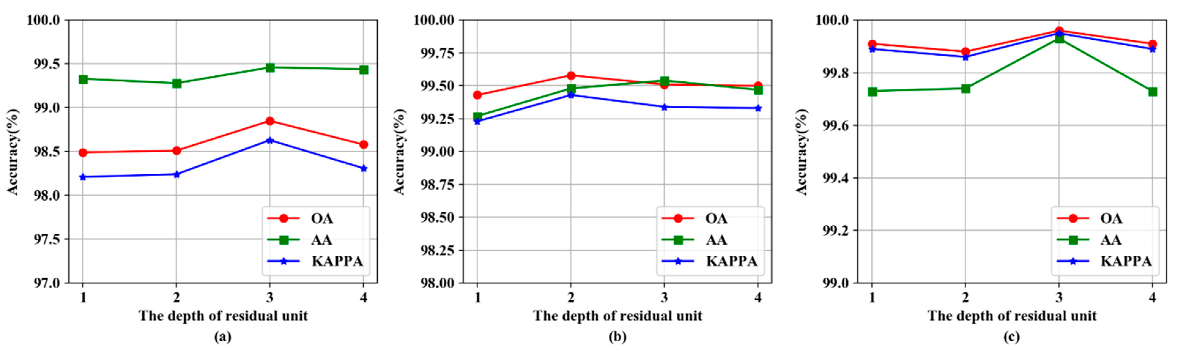
3.5. The Impact of Residual Unit Depth

In addition to the above factors, the depth of residual unit directly affects the feature extraction capability of the entire model. In other words, if the structure of the model is shallow, it would be unable to extract features effectively. The deeper structure is prone to gradient disappearance, but it cannot further improve the classification accuracy. In order to test the influence of the depth of residual units on the classification accuracy in three datasets, we chose the residual unit depth R to be 1, 2, 3 and 4 to conduct experiments.

The experimental results are shown in

Table 8. Model parameters for different residual unit depth (R) on three Data sets.

R	Indian Pines	Pavia University	Kennedy Space Center
1	21284	18750	17114
2	31036	29622	25306
3	40660	40366	33370
4	50252	51078	41402

and

Table 9. Training time, testing time, and OA for different residual unit depth (R) on three data sets.

R	Indian Pines			Pavia University			Kennedy Space Center
	Training Time(s)	Test Time(s)	OA (%)	Training Time(s)	Test Time(s)	OA (%)	Training Time(s)	Test Time(s)	OA (%)
1	725.25 ± 66.24	4.60 ± 0.04	98.49 ± 0.23	655.02 ± 50.04	14.13 ± 0.11	99.43 ± 0.25	755.43 ± 16.10	2.21 ± 0.03	99.91 ± 0.11
2	712.27 ± 24.13	4.59 ± 0.07	98.51 ± 0.28	739.40 ± 20.06	14.24 ± 0.05	99.58 ± 0.12	863.41 ± 13.49	2.25 ± 0.03	99.88 ± 0.12
3	714.28 ± 16.92	4.57 ± 0.03	98.85 ± 0.23	729.48 ± 5.88	14.26 ± 0.16	99.51 ± 0.20	850.34 ± 74.70	2.31 ± 0.01	99.96 ± 0.05
4	735.02 ± 28.17	5.74 ± 3.45	98.58 ± 0.36	638.42 ± 33.87	13.90 ± 0.08	99.50 ± 0.17	874.02 ± 55.47	2.34 ± 0.04	99.91 ± 0.08

. For the same dataset, each additional residual unit increases the parameters by about 10,000. On the Indian Pines dataset, the training and testing time did not change significantly with the increase of the number of residual units. In addition, with the number of residual units increasing, the training and testing times were gradually longer as a whole in Kennedy Space Center dataset, but the training and testing times were acceptable under the premise of obtaining the highest classification accuracy. As shown in Figure 7, the optimal accuracy was obtained when R was 3 for Indian Pines and Kennedy Space Center datasets. For the Pavia University dataset, when R was 2, the model acquired the highest classification accuracy.

4. Results and Discussion

In order to further measure the performance of the proposed classification model, we selected several typical classification models that became available in recent years. These include SVM-RBF [5], 1D-CNN [14], M3D-DCNN [20], SSRN [21], and pResNet [24]. Besides this, the same model using standard CNN (Std-CNN) instead of depth-wise separable convolution was also built. They were used in this study for detailed comparisons. More specifically, the SVM-RBF and 1D-CNN are spectral-based methods, and M3D-DCNN, pResNet, SSRN, Std-CNN, together with the present model, are spectral-spatial approaches. In order to ensure the fairness of the experiments, each group of experiments in three datasets were repeated 10 times. We uniformly used the space size that was determined in Section 3.3 of this section as the input of spectral-spatial model. The evaluation indicators OA, AA, Kappa coefficient, and F1-score are expressed in the form of "mean ± standard deviation".

In addition, we compared the proposed depth-separable convolution network (Des-CNN) with Std-CNN in detail to verify the feasibility and effectiveness of the depth-separable convolution approach for hyperspectral images classification.

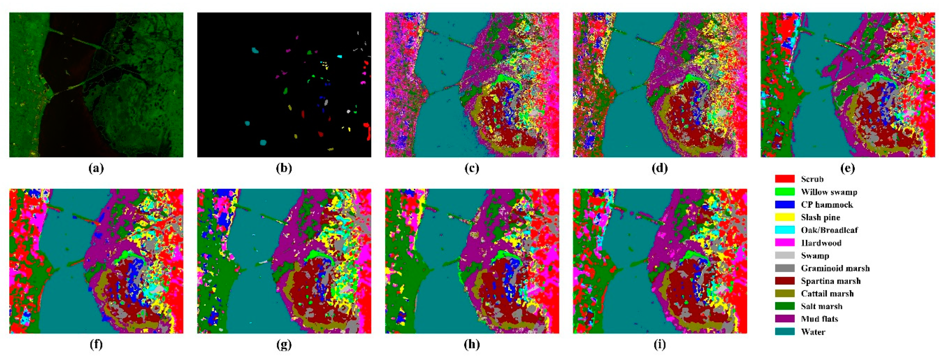
4.1. Comparison with Other Methods

The classification results for each of the methods are shown in

Table 10. Classification results of different methods for the Indian Pines data set.

Class	SVM-RBF	1D-CNN	M3D-DCNN	pResNet	SSRN	Std-CNN	Proposed
1	85.56	90.00	97.78	100.00	98.89	100.00	100.00
2	77.02	82.15	86.29	97.29	98.20	96.51	98.22
3	76.35	78.57	92.21	99.13	99.27	99.1	99.16
4	91.62	90.27	100.00	100.00	100.00	100.00	99.73
5	94.63	94.98	99.12	99.89	99.96	99.93	99.86
6	96.96	97.89	99.36	99.74	99.89	99.77	99.85
7	86.00	94.00	98.00	100.00	100.00	100.00	100.00
8	98.17	99.06	99.86	100.00	100.00	100.00	100.00
9	82.5	97.50	95.00	100.00	95.00	100.00	100.00
10	83.06	87.66	92.51	98.94	98.81	97.67	98.60
11	66.82	70.52	80.15	96.12	97.99	95.60	98.22
12	86.39	89.92	96.95	98.63	99.54	98.47	98.78
13	98.00	98.00	100.00	100.00	100.00	100.00	100.00
14	89.25	91.62	96.03	98.61	99.88	96.51	99.58
15	80.16	82.53	99.19	99.84	100.00	99.10	100.00
16	97.22	96.11	100.00	99.44	97.22	100.00	99.44
OA (%)	79.76 ± 0.68	82.99 ± 0.85	89.80 ± 1.36	98.09 ± 1.11	98.89± 0.44	97.67 ± 0.52	98.85 ± 0.23
AA (%)	86.86 ± 2.07	90.05 ± 0.92	95.78 ± 1.09	99.10 ± 0.55	99.04 ± 0.93	99.12 ± 0.15	99.46 ± 0.14
Kappa × 100	76.46 ± 0.78	80.17 ± 0.95	88.05 ± 1.57	97.59 ± 1.24	98.68± 0.52	97.24 ± 0.62	98.63 ± 0.27
F1-score × 100	76.41 ± 1.91	78.32± 1.70	90.66 ± 1.68	97.67 ± 1.01	97.47 ± 1.98	96.11 ± 1.21	97.79 ± 1.17

,

Table 11. Classification results of different methods for the Pavia University data set.

Class	SVM-RBF	1D-CNN	M3D-DCNN	pResNet	SSRN	Std-CNN	Proposed
1	86.01	87.48	90.84	98.86	99.56	99.81	99.83
2	90.25	89.87	96.01	99.55	99.68	99.64	99.71
3	84.47	84.92	91.72	98.58	99.02	99.71	99.67
4	95.10	95.93	98.01	98.84	98.20	97.92	97.74
5	99.42	99.78	99.92	99.94	99.87	99.79	99.83
6	89.96	88.66	97.84	99.69	99.99	100.00	99.90
7	93.19	92.27	96.65	99.51	100.00	100.00	100.00
8	85.11	81.92	93.27	99.15	99.16	99.35	99.22
9	99.92	99.79	99.57	99.92	99.42	99.45	99.41
OA (%)	89.70 ± 0.95	89.40 ± 0.98	95.31 ± 2.10	99.35 ± 0.17	99.53 ± 0.14	99.58 ± 0.29	99.58 ± 0.12
AA (%)	91.49 ± 0.45	91.18 ± 0.43	95.98 ± 1.31	99.34 ± 0.21	99.43 ± 0.16	99.52± 0.13	99.48 ± 0.15
Kappa × 100	86.36 ± 1.22	85.97 ± 1.23	93.76 ± 2.73	99.12 ± 0.23	99.37 ± 0.19	99.43 ± 0.39	99.43 ± 0.16
F1-score × 100	88.62 ± 0.68	88.24 ± 0.86	94.26 ± 1.96	99.16 ± 0.25	99.33 ± 0.25	99.44 ± 0.21	99.38 ± 0.16

and

Table 12. Classification results of different methods for the Kennedy Space Center data set.

Class	SVM-RBF	1D-CNN	M3D-DCNN	pResNet	SSRN	Std-CNN	Proposed
1	92.23	90.71	99.18	99.63	99.57	99.93	99.89
2	95.81	90.70	100.00	100.00	100.00	100.00	100.00
3	93.39	88.39	98.39	99.64	99.46	99.82	100.00
4	86.54	77.69	95.00	99.23	99.81	98.85	99.23
5	77.50	70.00	93.44	99.06	99.38	98.75	100.00
6	89.66	87.93	99.66	100.00	100.00	100.00	100.00
7	92.86	87.14	100.00	99.52	100.00	99.52	100.00
8	95.93	94.89	99.48	100.00	100.00	100.00	100.00
9	97.72	97.72	99.69	99.91	99.84	99.94	100.00
10	99.02	99.61	99.56	99.90	100.00	100.00	99.90
11	98.63	98.54	99.77	100.00	100.00	100.00	100.00
12	96.53	97.33	99.9	100.00	100.00	99.93	100.00
13	99.93	100.00	100.00	100.00	100.00	100.00	100.00
OA (%)	96.41 ± 0.30	95.67 ± 0.85	99.49 ± 0.26	99.87 ± 0.25	99.87 ± 0.10	99.93 ± 0.06	99.96 ± 0.05
AA (%)	93.52 ± 0.90	90.82 ± 0.85	98.77 ± 0.81	99.76 ± 0.35	99.85 ± 0.13	99.75 ± 0.21	99.93 ± 0.09
Kappa × 100	95.78 ± 0.35	94.91 ± 0.98	99.40 ± 0.31	99.85 ± 0.29	99.85 ± 0.12	99.92 ± 0.08	99.95 ± 0.06
F1-score × 100	90.53 ± 0.71	87.82 ± 1.14	98.32 ± 0.89	99.57± 0.80	99.59 ± 0.36	99.71 ± 0.29	99.85 ± 0.19

. First, it can be seen that the classification accuracy (OA, AA, Kappa values, and F1-score) of the model proposed in this paper are higher than those of other classification models (SVM-RBF, 1D-CNN, M3D-DCNN, pResNet) on all datasets. Specifically, in the Indian Pines data set, our model achieves roughly 17.48% higher mean OA than that of SVM-RBF, 1D-CNN, and about 3.66% higher than that of spectral-spatial models (M3D-CNN, Std-CNN, and pResNet). Clearly, the accuracies of SVM-RBF and 1D-CNN models using only spectral features are significantly lower than that of the spectral-spatial model. This implies that only spectral features were unable to achieve high classification accuracy. Then, it should be pointed out that the OA value of SSRN is only 0.04% higher than that of our model, but it has a higher standard deviation. In addition, the performance of 3D networks, such as M3D-DCNN and SSRN, seems to be limited, especially M3D-DCNN; its accuracy on the IP dataset is much lower than SSRN, Std-CNN, and our proposed depth-separable convolution model. From Table 10, the accuracy of No.2, 11 is only 86.29% and 80.15%, because the band information of the two samples is relatively similar, resulting in a misjudgment. Moreover, in the face of small sample surface features, the feature learning ability of the SSRN is insufficient, such as the accuracy of No.9, 16 is less than 98%, while our model is higher than 99.44%. Furthermore, the Std-CNN and the model in our proposal both get rid of the problem of small sample, and their classification accuracy is superior to other models on the same objects with small samples (No.1, 7, 9, 16), indicating that our model still has strong feature extraction capability under the condition of small sample data. Finally, for Indian Pines and Kennedy Space Center datasets, the OA, AA, Kappa values and F1-score of depth-wise separable convolution model are better than those of Std-CNN. However, for the Pavia University dataset, the OA and Kappa of the two models are equal, and the AA of the proposed model is only lower than Std-CNN 0.04%, but the gap is not obvious.

In addition, compared with other classification models, the standard deviation of our model results is the smallest, which further indicates that the proposed model ensures high accuracy while the classification effect is more stable.

Figure 8, Figure 9 and Figure 10 visualize the classification results of the different models in three datasets, as well as the false color images of original HSI and their corresponding ground-truth maps. It can be clearly seen from the classification map that only using spectral features for classification, such as SVM-RBF and 1D-CNN, will produce many noise points, but the spectral–spatial-based methods, M3D-CNN, pResNet, and proposed, overcome this shortcoming, especially our proposed model shows better classification effect. For example, in the Indian Pines data set, M3D-CNN and pResNet mistakenly labeled some pixels of Class 11 (Soybean-mintill) as Class 3 (Corn-mintill), while our proposed model correctly labeled them. Specifically, by comparing ground-truth maps, our model achieved a more accurate and smooth classification effect.

In the last part of the experiments, we compared the above CNN based 1D-CNN, M3D-CNN, pResNet, SSRN, Std-CNN, and our model in four aspects: floating point operations (FLOPs), the number of training parameters, training time, and test time. As shown in Figure 11, on three different datasets, the number of the parameters of our model constructed in this paper was far lower than that of other models. Among the other models, the pResNet had the most parameters, mainly because the structure of the model was extremely complex, which had approximately 40 layers. The parameters of the M3D-DCNN model were second only to those of pResNet. It consisted of 10 layers, and there were two three-dimensional multi-scale convolutional layers with the width being 4, which greatly increased the parameters and slowed down the classification speed. However, the 1D-CNN model was the shallowest, with only 5 layers. Its number of parameters was much lower than those of the M3D-DCNN or pResNet models. In addition, from

Table 13. Parameters, training time, and test time for different models, based on CNN, on the three data sets.

		1D-CNN	M3D-DCNN	pResNet	SSRN	Std-CNN	Proposed
Indian Pines	FLOPs(×106)	0.16	75.31	30.09	234.68	10.34	2.20
	Training time(s)	511.25	3380.23	1040.36	3519.76	772.93	714.28
	Test time(s)	1.29	8.49	8.01	16.75	4.62	4.57
Pavia University	FLOPs(×106)	0.08	54.26	42.16	168.71	17.95	3.01
	Training time(s)	541.52	1975.36	908.99	1759.32	684.71	739.40
	Test time(s)	1.81	29.72	26.52	60.46	14.11	14.24
Kennedy Space Center	FLOPs(×106)	0.15	39.25	20.44	137.74	5.87	1.20
	Training time(s)	509.26	2008.18	1396.61	2117.42	715.60	668.25
	Test time(s)	1.31	2.66	3.31	4.01	2.06	1.91

, the training time and test time of the proposed model were much less than those of M3D-DCNN and pResNet, but slightly higher than those of 1D-CNN. This was mostly because the 1D-CNN model only used the spectral features to complete the classification and lost the spatial information, so the time was slightly faster. The classification accuracy of the model was lower, however.

On the other hand, we can also observe in Table 13 that the FOLPs of 1D-CNN is the lowest, only 0.16M. This is because 1D convolution operation is relatively simple in the process of exploring spectral information, so the ability of feature learning is limited. However, the FLOPs of 3D-CNN and SSRN are as high as 234.68M and 75.31M, respectively, especially the SSRN is about 100 times that of our model. The reason is that the 3D convolution networks need a great number of floating-point calculations in the training process for feature learning. In contrast, the computational burden of 2D networks is insignificant, such as pResNet and Std-CNN. Especially pResNet with more parameters has fewer FLOPs than 3D networks. Nevertheless, the performance of the 3D network and the standard 2D network did not show advantages, mainly due to the excessive redundant parameters in network limited the feature representation. Finally, it should be noted that the parameters and FLOPs of Std-CNN are approximately 6 times the depth-separable convolution model in the same data set, which indicates that the computational cost of the model we build is lower.

In short, in pursuit of high precision, the model in this paper is superior to other models in terms of the number of parameters, training time, and testing time. In addition, Depth-wise separable convolution is feasible and has some advantages such as low cost, simple structure, and accuracy compared with standard convolution. In practical application, this lightweight framework does not require too much computer hardware platform.

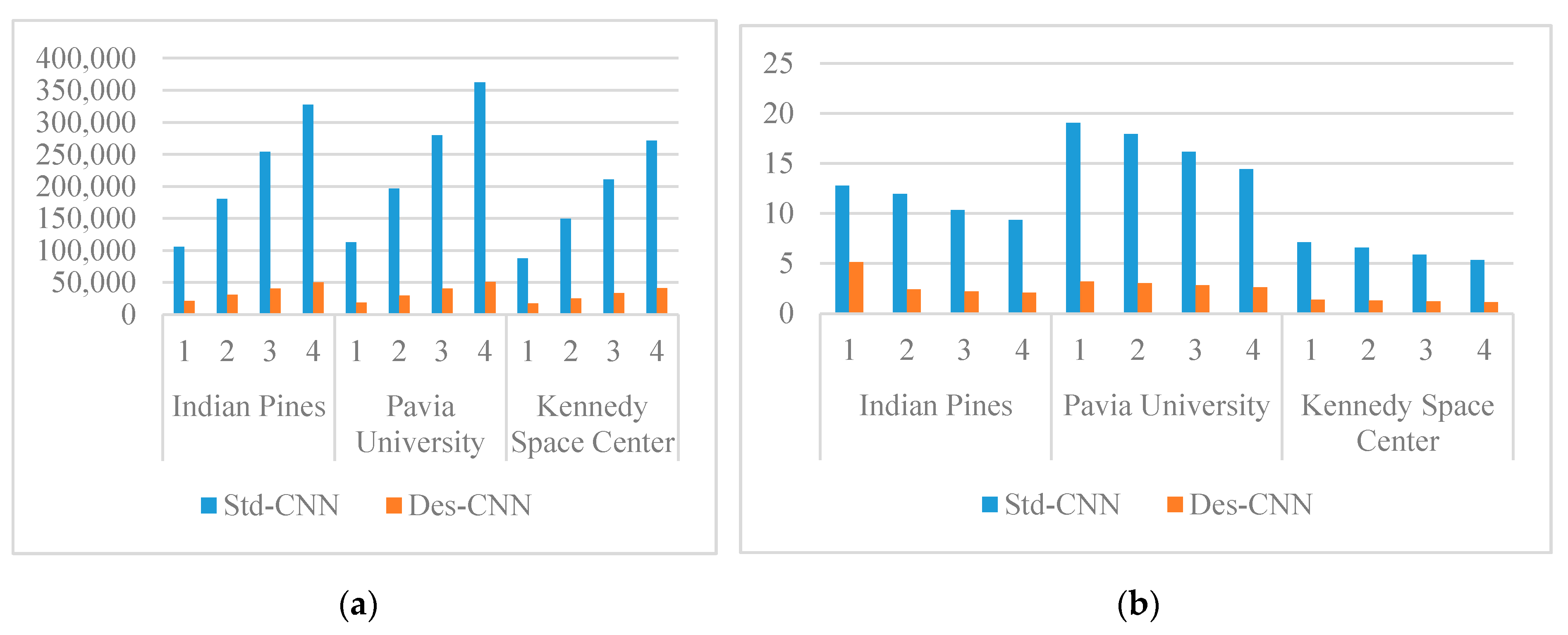
4.2. Effectiveness Analysis to Depth-Separable Convolution

In this part, we compared Std-CNN with the proposed depth-separable convolution network (Des-CNN) in detail to verify the feasibility and effectiveness of the depth-separable convolution approach for hyperspectral images classification. The OA and F1-score of the two models on different data sets are recorded in

Table 14. The Overall (OA) classification accuracy (%) for Standard CNN and the proposed model on three HSI datasets.

		Indian Pines		Pavia University		Kennedy Space Center
		Std-CNN	Des-CNN	Std-CNN	Des-CNN	Std-CNN	Des-CNN
Spatial Size	5 × 5	89.04 ± 0.81	94.63 ± 0.97	96.48 ± 0.99	97.23 ± 0.69	99.54 ± 0.24	99.75 ± 0.12
	7 × 7	94.36 ± 0.94	97.31 ± 0.55	98.33 ± 0.44	98.61 ± 0.31	99.80 ± 0.11	99.95 ± 0.05
	9 × 9	97.42 ± 0.57	98.63 ± 0.38	99.48 ± 0.11	99.25 ± 0.41	99.96 ± 0.05	99.96 ± 0.08
	11 × 11	97.87 ± 0.39	98.85 ± 0.23	99.46 ± 0.25	99.45 ± 0.19	99.97 ± 0.06	99.93 ± 0.07
	13 × 13	98.01 ± 0.46	98.39 ± 0.36	99.54 ± 0.25	99.46 ± 0.19	99.96 ± 0.05	99.87 ± 0.28
	15 × 15	97.68 ± 0.34	98.00 ± 0.44	99.57 ± 0.16	99.64 ± 0.13	99.99 ± 0.02	99.99 ± 0.03
Initial Convolution Kernels Number	16	97.37 ± 0.42	98.38 ± 0.65	99.36 ± 0.24	99.07 ± 0.47	99.93 ± 0.09	99.94 ± 0.09
	24	97.63 ± 0.50	98.46 ± 0.53	99.50 ± 0.39	99.33 ± 0.42	99.95 ± 0.04	99.91 ± 0.07
	32	97.79 ± 0.43	98.60 ± 0.40	99.51 ± 0.26	99.43 ± 0.27	99.89 ± 0.11	99.96± 0.05
	38	97.87 ± 0.39	98.85± 0.23	99.54 ± 0.25	99.46 ± 0.19	99.96 ± 0.05	99.96 ± 0.08
	42	97.68 ± 0.48	98.63 ± 0.29	99.36 ± 0.64	99.51± 0.20	99.96 ± 0.05	99.94 ± 0.04
Residual Unit Depth	1	98.74 ± 0.44	98.49 ± 0.23	99.57 ± 0.13	99.43 ± 0.25	99.92 ± 0.08	99.91 ± 0.11
	2	98.29 ± 0.24	98.51 ± 0.28	99.44 ± 0.53	99.58 ± 0.12	99.94 ± 0.06	99.88 ± 0.12
	3	97.87 ± 0.39	98.85 ± 0.23	99.54 ± 0.25	99.51 ± 0.20	99.89 ± 0.11	99.96 ± 0.05
	4	96.58 ± 0.67	98.58 ± 0.36	99.37 ± 0.28	99.50 ± 0.17	99.87 ± 0.10	99.91 ± 0.08

and

Table 15. F1-score × 100 for Standard CNN and the proposed model on three HSI datasets.

		Indian Pines		Pavia University		Kennedy Space Center
		Std-CNN	Des-CNN	Std-CNN	Des-CNN	Std-CNN	Des-CNN
Spatial size	5 × 5	91.24 ± 1.21	94.45 ± 1.14	96.31 ± 0.73	96.95 ± 0.90	98.67 ± 0.70	99.75 ± 0.12
	7 × 7	94.91 ± 0.92	96.91 ± 1.01	97.95 ± 0.42	98.29 ± 0.39	99.33 ± 0.41	99.80 ± 0.14
	9 × 9	97.19 ± 0.96	98.35 ± 0.85	99.30 ± 0.17	99.13 ± 0.35	99.88 ± 0.12	99.84 ± 0.31
	11 × 11	96.11 ± 1.21	97.79 ± 1.17	99.35 ± 0.25	99.31 ± 0.21	99.92 ± 0.19	99.78 ± 0.17
	13 × 13	96.19 ± 1.57	96.20 ± 1.56	99.41 ± 0.20	99.31 ± 0.23	99.96 ± 0.05	99.57 ± 0.79
	15 × 15	94.81 ± 1.95	96.04 ± 1.36	99.40 ± 0.16	99.47 ± 0.11	99.94 ± 0.12	99.93 ± 0.18
Initial Convolution Kernels Number	16	96.68 ± 1.32	97.87 ± 1.23	99.20 ± 0.20	98.99 ± 0.38	99.71 ± 0.40	99.81 ± 0.37
	24	96.96 ± 0.96	97.44 ± 1.01	99.39 ± 0.33	99.22 ± 0.31	99.79 ± 0.19	99.91 ± 0.07
	32	96.93 ± 0.99	96.84 ± 1.76	99.51 ± 0.26	99.26 ± 0.32	99.61 ± 0.32	99.85 ± 0.19
	38	96.11 ± 1.21	97.79 ± 1.17	99.41 ± 0.20	99.31 ± 0.23	99.88 ± 0.12	99.84 ± 0.31
	42	96.51 ± 0.91	97.52 ± 1.79	99.24 ± 0.61	99.42 ± 0.17	99.82 ± 0.21	99.76 ± 0.16
Residual Unit Depth	1	97.04 ± 1.41	96.02 ± 1.90	99.34 ± 0.18	99.14 ± 0.24	99.76 ± 0.25	99.59 ± 0.57
	2	96.04 ± 1.77	96.28 ± 1.68	99.30 ± 0.39	99.58 ± 0.12	99.94 ± 0.06	99.88 ± 0.12
	3	96.11 ± 1.21	97.79 ± 1.17	99.41 ± 0.20	99.42 ± 0.17	99.89 ± 0.11	99.85 ± 0.19
	4	96.25 ± 1.39	98.00 ± 0.79	99.39 ± 0.24	99.34 ± 0.36	99.49 ± 0.39	99.91 ± 0.08

, respectively. It can be seen that compared with Std-CNN, the OA and F1-score performance of the Des-CNN on Indian Pines data set achieved higher accuracy. Specifically, most of the results of Des-CNN exceeded Std-CNN for the same threshold under the same hyper-parameter, especially in the case of the small threshold (Spatial Size = 5, 7; and Initial Convolution Kernels Number are 16, 24), the difference was more obvious. However, the performance of Des-CNN on the Pavia University and Kennedy Space Center data sets was slightly worse than that of Std-CNN. Under the same configuration, the accuracy (OA, FLOPs) of Des-CNN was slightly lower than those of Std-CNN, but this difference was less than 1%.

Besides accuracy, the complexity and computational load of the model are another important consideration. Since the standard convolution and depth-separable convolution appeared in the residual unit, the complexity of the network framework was mainly affected by the depth of the residual unit. The training parameters and FLOPs of Std-CNN and Des-CNN at different residual unit depths are shown in Figure 12, respectively. Obviously, the training parameters and FLOPs of Std-CNN were much higher than those of Des-CNN under the same configuration. From Figure 12a, the training parameters of Des-CNN under different residual units on the three data sets were all lower than 50,000, while the parameters of Std-CNN were mostly more than 10,000. From Figure 12b, the FLOPs of Std-CNN were higher than 5M, and even more than 10M on Indian pines and Pavia University, while the flops of Des-CNN were less than 5M on three datasets.

From the above analysis, compared with Std-CNN, Des-CNN constructed by depth-separable convolution achieved competitive results on Indian Pines data set and was slightly insufficient on Pavia University and Kennedy Space Center data sets. However, the difference was very small. In addition, the model complexity of Des-CNN was significantly better than that of Std-CNN on three data sets. Consequently, it is sufficient to demonstrate that depth-separable convolution is feasible for hyperspectral classification. Compared with Std-CNN, the proposed model is more lightweight, and it is more satisfied with limited computer hardware devices in reality.

5. Conclusions

In this paper, a lightweight model for HSI classification was constructed and discussed. Results of experiments show that it has fewer parameters and faster classification speed. In the first layer of the model, a 1 × 1 convolution kernel was used to re-combine the input channels of HSI and realize the cross-channel information integration. This reduced the number of spectral channels. Next, the spatial-spectral features were extracted by residual unit of the middle layer. At the end of executing the model, a combination of a 1 × 1 filter and a global average pooling layer was used to replace the full connection layer to complete the final classification. That further reduced the number of model parameters and sped up the classification while ensuring the accuracy.

In the experiments, the effect of space size, the number of initial convolution kernels, and the depth of residual units on the classification accuracy were first analyzed. Then, we further compared experimental results with results from other classification models. The experimental result shows that the proposed model reduced the number of parameters to a large extent and had a faster classification speed while ensuring higher accuracy. In addition, the proposed model has powerful feature extraction capabilities, because it still shows high classification accuracy on small sample data. Finally, we continued to explore the impact of the model that was constructed by standard convolution and depth-wise separable convolution on classification accuracy, the number of parameters and FLOPs. The experimental results showed that depth-separable convolution is feasible for hyperspectral classification. Compared with Std-CNN, the proposed model is more lightweight, and it is more satisfied with limited computer hardware devices in reality.

For future research work, three-dimensional convolution will be used to extract spectral features, and two-dimensional convolution will fuse spatial-spectral features, introducing density connection to speed up the flow of feature information, further reduce the training and testing time of the model, and accelerate the convergence of the model so as to build a more rapid and effective HSI classification model.

References

1. Nakhostin, S.; Clenet, H.; Corpetti, T.; Courty, N. Joint anomaly detection and spectral unmixing for planetary Hyperspectral Images. IEEE Geosci. Remote Sens. 2016, 54, 6879–6894. [Google Scholar] [CrossRef] [Green Version]
2. Torrecilla, E.; Stramski, D.; Reynolds, R.A.; Millán-Núñez, E.; Piera, J. Cluster analysis of hyperspectral optical data for discriminating phytoplankton pigment assemblages in the open ocean. Remote Sens. Environ. 2011, 115, 2578–2593. [Google Scholar] [CrossRef] [Green Version]
3. Pan, Z.; Glennie, C.L.; Fernandez-Diaz, J.C.; Legleiter, C.J.; Overstreet, B. Fusion of LiDAR orthowaveforms and hyperspectral imagery for shallow river bathymetry and turbidity estimation. IEEE Geosci. Remote Sens. 2016, 54, 4165–4177. [Google Scholar] [CrossRef]
4. Li, C.H.; Hun, C.C.; Taur, J.S. An effective feature selection method for hyperspectral image classification based on genetic algorithm and support vector machine. Knowl. Based Syst. 2011, 24, 40–48. [Google Scholar] [CrossRef]
5. Kuo, B.C.; Ho, H.H.; Li, C.H. A kernel-based feature selection method for SVM with RBF kernel for hyperspectral image classification. IEEE J. Sel. Top. Appl. Earth Obs. Remote Sens. 2013, 7, 317–326. [Google Scholar]
6. Zhu, Z.; Jia, S.; He, S.; Sun, Y.; Ji, Z.; Shen, L. Three-dimensional gabor feature extraction for hyperspectral imagery classification using a memetic framework. Inf. Sci. 2015, 298, 274–287. [Google Scholar] [CrossRef]
7. Fauvel, M.; Dechesne, C.; Zullo, A.; Ferraty, F. Fast forward feature selection of hyperspectral images for classification with gaussian mixture models. IEEE J. Sel. Top. Appl. Earth Obs. Remote Sens. 2015, 8, 2824–2831. [Google Scholar] [CrossRef]
8. LeCun, Y.; Bottou, L.; Bengio, Y.; Haffner, P. Gradient-based learning applied to document recognition. Proc. IEEE Inst. Electr. Electron Eng. 1998, 86, 2278–2324. [Google Scholar] [CrossRef] [Green Version]
9. Simonyan, K.; Zisserman, A. Very deep convolutional networks for large-scale image recognition. arXiv 2015, arXiv:1409.1556. [Google Scholar]
10. Howard, A.G.; Zhu, M.; Chen, B.; Kalenichenko, D.; Wang, W.; Weyand, T.; Adam, H. MobileNets: Efficient convolutional neural networks for mobile vision applications. arXiv 2015, arXiv:1704.04861. [Google Scholar]
11. Abdel-Hamid, O.; Mohamed, A.R.; Jiang, H.; Penn, G. Applying Convolutional Neural Networks Concepts to Hybrid NN-HMM Model for Speech Recognition. In Proceedings of the International Conference on Acoustics, Speech, and Signal Processing (ICASSP), Kyoto, Japan, 25–30 March 2012; pp. 4277–4280. [Google Scholar]
12. Girshick, R.; Donahue, J.; Darrell, T.; Malik, J. Rich feature hierarchies for accurate object detection and semantic segmentation. Proc. IEEE Conf. Comput. Vis. Pattern Recognit. 2014, 580–587. [Google Scholar] [CrossRef] [Green Version]
13. Long, J.; Shelhamer, E.; Darrell, T. Fully convolutional networks for semantic segmentation. IEEE Trans. Pattern Anal. Mach. Intell. 2014, 39, 640–651. [Google Scholar]
14. Hu, W.; Huang, Y.; Wei, L.; Zhang, F.; Li, H. Deep convolutional neural networks for hyperspectral image classification. J. Sens. 2015, 2015, 258619. [Google Scholar] [CrossRef] [Green Version]
15. Makantasis, K.; Karantzalos, K.; Doulamis, A.; Doulamis, N. Deep supervised learning for hyperspectral data classification through convolutional neural networks. In Proceedings of the International Geoscience and Remote Sensing Symposium (IGARSS), Milan, Italy, 26–31 July 2015; pp. 4959–4962. [Google Scholar]
16. Zhang, H.; Li, Y.; Zhang, Y.; Shen, Q. Spectral-spatial classification of hyperspectral imagery using a dual-channel convolutional neural network. Remote Sens. Lett. 2017, 8, 438–447. [Google Scholar] [CrossRef] [Green Version]
17. Yu, S.; Jia, S.; Xu, C. Convolutional neural networks for hyperspectral image classification. Neurocomputing 2017, 219, 88–89. [Google Scholar] [CrossRef]
18. Lee, H.; Kwon, H. Contextual deep CNN based hyperspectral classification. In Proceedings of the International Geoscience and Remote Sensing Symposium (IGARSS), Beijing, China, 10–15 July 2016; pp. 3322–3325. [Google Scholar]
19. Szegedy, C.; Liu, W.; Jia, Y.; Sermanet, P.; Reed, S.; Anguelov, D.; Rabinovich, A. Going deeper with convolutions. Proc. IEEE Conf. Comput. Vis. Pattern Recognit. 2015, 1–9. [Google Scholar] [CrossRef] [Green Version]
20. He, M.; Li, B.; Chen, H. Multi-scale 3D deep convolutional neural network for hyperspectral image classification. Proc. IEEE Int. Conf. Image Process. 2017, 3904–3908. [Google Scholar] [CrossRef]
21. Zhong, Z.; Li, J.; Luo, Z.; Chapman, M. Spectral–spatial residual network for hyperspectral image classification: A 3-D deep learning framework. IEEE Trans. Geosci. Remote Sens. 2018, 56, 847–858. [Google Scholar] [CrossRef]
22. Wang, W.; Dou, S.; Jiang, Z.; Sun, L. A fast dense spectral spatial convolution network framework for hyperspectral images classification. Remote Sens. 2018, 10, 1068. [Google Scholar] [CrossRef] [Green Version]
23. Gao, H.; Yang, Y.; Li, C.; Zhang, X.; Zhao, J.; Yao, D. Convolutional neural network for spectral–spatial classification of hyperspectral images. Neural. Comput. 2018, 31, 8997–9012. [Google Scholar] [CrossRef]
24. Paoletti, M.E.; Haut, J.M.; Fernandez-Beltran, R.; Plaza, J.; Plaza, A.J.; Pla, F. Deep pyramidal residual networks for spectral–Spatial hyperspectral image classification. IEEE Trans. Geosci. Remote Sens. 2019, 57, 740–754. [Google Scholar] [CrossRef]
25. Han, D.; Kim, J.; Kim, J. Deep pyramidal residual networks. Proc. IEEE Conf. Comput. Vis. Pattern Recognit. 2017, 6307–6315. [Google Scholar] [CrossRef] [Green Version]
26. Chollet, F. Xception: Deep Learning with depthwise separable convolutions. arXiv 2017, arXiv:1610.02357. [Google Scholar]
27. He, K.; Zhang, X.; Ren, S.; Sun, J. Deep residual learning for image recognition. Proc. IEEE Conf. Comput. Vis. Pattern Recognit. 2016, 770–778. [Google Scholar]
28. Nair, V.; Hinton, G.E. Rectified linear units improve restricted Boltzmann machines. In Proceedings of the 27th International Conference on International Conference on Machine Learning (ICML), Haifa, Israel, 21–24 June 2010; Omnipress: Madison, WI, USA, 2010; pp. 807–814. [Google Scholar]
29. Ioffe, S.; Szegedy, C. Batch normalization: Accelerating deep network training by reducing internal covariate shift. In Proceedings of the 32nd International Conference on International Conference on Machine Learning, Paris, France, 6–11 July 2015; pp. 448–456. [Google Scholar]
30. Donoho, D.L. High-dimensional data analysis: The curses and blessings of dimensionality. AMS Math Chall. Lect. 2000, 1, 32. [Google Scholar]
31. Lin, M.; Chen, Q.; Yan, S. Network in network. arXiv 2013, arXiv:1312.4400. [Google Scholar]
32. He, K.; Zhang, X.; Ren, S.; Sun, J. Delving deep into rectifiers: Surpassing human-level performance on ImageNet classification. In Proceedings of the International Conference on Computer Vision (ICCV), Santiago, Chile, 13–16 December 2015; pp. 1026–1034. [Google Scholar] [CrossRef] [Green Version]
Figure 1. The process of depth-wise separable convolution. This process includes depth-wise convolution, and 1 × 1 convolution.
Remotesensing 12 03408 g001
Figure 2. The structure of basic residual unit. Its execution order is: Conv→ batch normalization (BN)→rectified linear unit (ReLU)→Conv→BN.
Remotesensing 12 03408 g002
Figure 3. The structure of pyramid residual unit. Unlike a basic residual unit, the last ReLU layer was deleted, and BN was required before the first convolution operation in this unit.
Remotesensing 12 03408 g003
Figure 4. The overall structure of proposed model for hyperspectral images (HSI) classification.
Remotesensing 12 03408 g004
Figure 5. Accuracy of three data sets with different spatial sizes: (a) Indian Pines; (b) Pavia University; (c) Kennedy Space Center.
Remotesensing 12 03408 g005
Figure 6. Accuracy of three data sets with number of initial convolution kernels: (a) Indian Pines; (b) Pavia University; (c) Kennedy Space Center.
Remotesensing 12 03408 g006
Figure 7. Accuracy of three data sets with depth of residual unit: (a) Indian Pines; (b) Pavia University; (c) Kennedy Space Center.
Remotesensing 12 03408 g007
Figure 8. Classification maps of the different models for the Indian Pines data set: (a) false color image; (b) ground-truth map; (c) SVM-RBF; (d) 1D-CNN; (e) M3D-CNN; (f) pResNet; (g) SSRN; (h) Std-CNN; (i) proposed.
Remotesensing 12 03408 g008
Figure 9. Classification maps of the different models for the Pavia University data set: (a) false color image; (b) ground-truth map; (c) SVM-RBF; (d) 1D-CNN; (e) M3D-CNN; (f) pResNet; (g) SSRN; (h) Std-CNN; (i) proposed.
Remotesensing 12 03408 g009
Figure 10. Classification maps of the different models for the Kennedy Space Center data set: (a) false color image; (b) ground-truth map; (c) SVM-RBF; (d) 1D-CNN; (e) M3D-CNN; (f) pResNet; (g) SSRN; (h)Std-CNN; (i) proposed.
Remotesensing 12 03408 g010
Figure 11. The number of trainable parameters of the different models.
Remotesensing 12 03408 g011
Figure 12. Training parameters and FLOPs (×106) of Std-CNN and Des-CNN under different residual unit depths: (a) the number of training parameters; (b) the number of FLOPs.
Remotesensing 12 03408 g012