Statistical Analysis of 1996–2017 Ozone Profile Data Obtained by Ground-Based Microwave Radiometry

Abstract

Trends in the ozone layer remain among the major problems of the atmosphere physics; thus, results of measurements of the ozone altitude distribution (profile), carried out in the same place and via the same method, are very important. This paper presents the results of the statistical analysis of ensembles of ozone profiles obtained from ground-based microwave radiometry data acquired at the P.N. Lebedev Physical Institute over a period of two decades (1996–2017). The data collected show the significant difference between monthly mean statistical parameters of ozone profiles of the decades 1996–2006 and 2007–2017. The main and unexpected result is the drastic decrease in monthly root-mean-square (rms) variances of ozone profiles over Moscow above 30 km in cold months of the decade 2007–2017 (if compared to the variances in the decade 1996–2006) with the maximum fall by 46% at 39 km in February monthly mean variances. The decade change of variances obtained by averaging over all nine months in the analysis (from September to May) has the same decrease with maximum fall by 25% at 38 km. Additionally, significant decade changes were revealed in other monthly mean statistical parameters: probability density of ozone profile variances, inter-altitude covariance and correlation functions, and time covariance and correlation—as well as their frequency spectra. The decade change of the ozone profile obtained by averaging over the nine months appeared much less significant: the decrease by 5.7% at the altitude of 19 km (with 1.5% sampling error), minor decrease by 2.6% (with sampling error 1.5%) in the profile maximum at 37 km, and increases of 1.7% at 28 km and 2.5% at 47 km (with sampling errors 1.7%)—lower and higher of this maximum. In addition to that, the corresponding averaged mean total column (integral) ozone content above 20 km remained practically unchanged: 4.61 g/m² for decade 1996–2006 as compared to 4.58 g/m² for 2007–2017. Possible explanations of revealed offsets are proposed and discussed.

1. Introduction

The depletion of the ozone layer, which protects life on the Earth from the harmful solar UVB radiation by anthropogenic chlorine and bromine, remains among the major problems. As mentioned in [1], the Montreal Protocol has been successful, and the decline in ozone in the upper stratosphere stopped around in 1996–1997 [2], and in 2014, the increase in ozone was observed; however, it was statistically significant only in the upper stratosphere (around 42 km or 2 hPa), but not at lower levels, nor for total ozone columns [2]. More recent data of satellite and ground-based measurements of ozone profiles published in recent years (see in a comprehensive review [2]) demonstrate significant ozone increases in the upper stratosphere, between 35 and 48 km altitude (5 and 1 hPa). Closer to 2 hPa (42 km), the ozone was increasing by about 1.5 % per decade in the tropics, and by 2 to 2.5 % per decade in the 35° to 60° latitude zones of both hemispheres. At levels below 35 km (5 hPa), trends in the ozone layer from 2000 to 2016 were smaller and not statistically significant. This study confirms positive trends of the upper stratospheric ozone reported in [1]. The observed trends of profiles are consistent with expectations from chemistry climate model simulations.

In recent years, multiple studies of the ozone layer were related to the influence of planetary waves, polar stratospheric vortex, and sudden stratospheric warmings on the formation of ozone fields and other trace gases in the atmosphere [3,4,5]. The quantitative study was applied to determine numerical models of the atmosphere dynamics, chemistry, and thermal regime that describe the effects of stratospheric warmings on stratosphere ozone and other trace gases [3,4]. Such models are developed on the basis of experimental data on changes in the ozone vertical distribution not only in the upper and lower stratosphere, where ozone is the most sensitive to the anthropogenic pollution with chlorofluorocarbons [1], but also in the middle stratosphere layers (10 mbar, height ~30 km), where the ozone is expected to decrease due to the higher nitrogen content in the stratosphere [6]. To date, the origin of the ozone depletion has not been sufficiently studied, and it is sometimes unpredictable, such as “the Arctic ozone hole” in the spring of 2011 [7]. So, as mentioned in [2], a thorough analysis of possible drifts and differences between various data sources is still required. Ongoing quality observations from multiple independent platforms are the key for verifying that recovery of the ozone layer continues as expected [2].

In view of these studies, the results presented herein of the statistical analysis of the two-decade (1996–2017) ensemble of profiles of the ozone volume mixing ratio obtained in the same place and with the same method are very important. The geographical position of Moscow allows the observation of air masses of very different origins including, in particular, the air of the polar stratospheric vortex when it appears over Moscow that leads to strong variations of the ozone profile, especially in periods of violent stratospheric disturbances and sudden midwinter stratospheric warmings that occurred in the past two decades. Additionally, strong ozone variations can be related to planetary waves.

2. Equipment, Measurements, and Data Processing

Our study is based on data of the ground-based remote sensing of the atmospheric ozone at millimeter waves (microwaves), which is an effective way to study the ozone vertical distribution [8,9,10,11,12]. The monitoring of brightness temperatures of the atmospheric ozone thermal emission at frequencies of its spectral line centered at 142.175 GHz was carried out at the P.N. Lebedev Physical Institute of the Russian Academy of Sciences (LPI) (Moscow, 55°45′N, 37°37′E) in 1996–2017.

Amplitude-switching heterodyne receiver of the LPI ozone spectrometer (ozonometer) is based on the planar Schottky diode mixer. Single sideband receiver noise temperature is about 1500 K without cooling and about 700 K under liquid nitrogen cooling. Typically, room temperature operation was used for regular day-time ozone measurements in 1996–2017. Two filter-bank spectrum analyzers were used (80 spectral channels in the frequency bandwidth of 283 MHz from 1996 to 2007 [13] and 96 channels in the bandwidth of 475 MHz since 2007 [14]). The width of their channels increased in five steps from 0.2/0.1 MHz in the ozone line center to 20 MHz at wings, so the devices were adapted to the line contour [9,10]. In 2005–2006, ozone observations were carried out with both spectrum analyzers to compare spectra and retrieved ozone profiles obtained with the filter-banks. This provided continuity of ozone measurements in two decades. The Gaussian antenna pattern of the ozonometer is of 1.5° HPFW without side-lobes above −30 dB. Brightness temperature of the atmosphere measured in broadband (~0.6 GHz) channel of the instrument was used to determine tropospheric loss due to molecular oxygen and water. Two external blackbody loads (at room and liquid nitrogen temperatures) were used for calibration of the ozonometer.

All measurements were carried out in the daytime. Duration of the measurements was 1–3 h depending on weather conditions. In fact, our ground-based microwave ozone measurements (unlike lidar measurements) are possible for wide weather conditions (haze, fog, clouds, snow) except for drizzle and rain when tropospheric loss for zenith angle of 60 º was more than approximately 5 dB. Mean number of measurements used for the statistical analysis was 15–20 per month (typically, all working days except for ones with bad weather). Data of night-time observations were too rare for the statistical analysis (about 50 nights) and were not included in the paper.

Data processing included recalculating unit 200 s ozone spectra outside the troposphere (multiplying them by the tropospheric loss, corresponding systematic errors of 1–1.5% were vanished in the differential version of the presented below algorithm) and averaging the spectra (about 20 ones for good weather) to increase the signal-to-noise ratio.

This microwave technique gives day-and-night measurements of the ozone profile at altitudes from approximately 15 to 70 km (up to 100 km at night) [10] and is the most suitable one for long-term ground-based monitoring of the ozone profile in the stratosphere and lower mesosphere.

The LPI microwave ozonometer that provides data of systematic measurements of the vertical ozone profile in the stratosphere was included in the global ozonometric network in the framework of international programs DYANA, CRISTA/MAHRSI, and SOLVE. As an important milestone in the development of this network, the first simultaneous microwave observations of the ozonosphere from different points were carried out at the LPI and at Onsala Space Observatory (OSO, Sweden) in 1988–1990 [15].

The statistical analysis is based on the radiometric ozone monitoring in 1996–2017 (2096 vertical ozone profiles over Moscow with 1 km height step). The data were obtained for nine months from September to May, including 1169 profiles in the 1996–2006 decade and 927 ones in the 2007–2017 decade. These long measurements carried out in the same place make it possible to study long-term changes in ozonosphere. Diurnal variations are absent in the data obtained approximately in the same hours of daytime; however, the effect of seasonal variations on statistical parameters was studied and taken into account. Nine data sets—for September (59 elements), October (134), November (248), December (337), January (374), February (357), March (341), April (184), and May (62) (for autumn, winter and spring seasons)—were extracted from the data. Summer months were not included in the analysis (measurements were sparse and not enough informative because of very low level of summer ozone variations). To study long-term changes, the data extracted for each month were divided into two ensembles of 1996–2006 and 2007–2017 decades.

Ozone profile retrieval from measured spectra of brightness temperatures is based on solving the corresponding nonlinear integral equation with the iterative algorithm developed in [16] an successfully applied in [9,10], where at each step of iterations the corresponding Fredholm integral equation of the 1st kind is solved with the Tikhonov’s method of generalized discrepancy [17] that uses general a priori information on the smoothness of the exact solution. Unlike methods based on the “common wisdom” regularization [18,19,20] or the formal statistical regularization [21] of this ill-posed problem, this method is mathematically consistent and provides the convergence to the exact solution in the Sobolev’s functional class ${\mathrm{W}}_2^1$ (see details in Appendix A). This approach was firstly proposed in the inverse problem of limb-viewing satellite microwave ozone profiling [22,23]. In this paper, we demonstrate results of this method in the study of long-term offsets in mean ozone profiles, their inter-altitude, and time variations.

3. Statistical Analysis

3.1. Statistical Parameters and Method of Errors Correction

Based on above-described data ensembles of ozone profiles U(h) retrieved by solving algorithm (A9), see Appendix A, various statistical parameters were calculated: mean ozone profiles $<U(h)>$, profiles of variances ${\sigma }^2(h)=<{[U(h)-<U(h)>]}^2>$ and rms deviations of ozone profile $\sigma (h)$, probability density of ozone profile variations $P(U\left(h\right)-<U\left(h\right)>)$, inter-altitude covariance functions $B(h_1,h_2)=<[U(h_1)-<U(h_1)>][(U(h_2)-<U(h_2)>]>$, and inter-altitude correlation functions $R(h_1,h_2)=B(h_1,h_2)/\sqrt{B(h_1,h_1)B(h_2,h_2)}$. For time intervals $\tau$ much less than the typical time of seasonal variations, time covariance functions $B_t(h,\tau )=<[U(h,t)-<U(h)>][(U(h,t+\tau )-<U(h)>]>$, time correlation functions $R_t(h,\tau )=B_t(h,\tau )/{\sigma }^2(h)=B_t(h,\tau )/B(h,h)$, and their frequency spectra $S_B(h,f)={\displaystyle {\int }_{\mathsf{\Delta }\tau }{B}_t(h,\tau )}\exp (-2\pi if\tau )d\tau$,$S_R(h,f)={\displaystyle {\int }_{\mathsf{\Delta }f}{R}_t(h,\tau )}\exp (-2\pi if\tau )d\tau$ were determined. Available dimensions of data ensembles provided a high enough accuracy of these estimations.

It is worth mentioning that results of the numerical simulation [9,10] obtained for various simulated (typical and extreme) profiles gave the estimation of the retrieval accuracy in C-metric, but this simulation was unsuitable to obtain their statistical estimations. Now it appears possible to realize the numerical simulation according the steps (a)–(e) of the scheme described in the Appendix A after the formula (A11), where ensembles of the retrieved ozone profiles are used as preset ones that give us the set {U₂(h)} of secondary retrieved profiles.

Let us write these profiles as sum U₂(h) = U(h) + ΔU(h) + δU(h) where ΔU(h) is the systematic error and δU(h) is random error with zero mean value. Then, one can obtain statistical parameters of the retrieval errors of the method itself—systematic errors $\mathsf{\Delta }U(h)=<U_2(h)-U(h)>$ and the dispersion of random errors ${\sigma }_{\delta U}^2(h)=<{[U_2(h)-U(h)-\mathsf{\Delta }U(h)]}^2>$. Here, we propose to use these parameters to clear (correct) some statistical parameters of initially retrieved ozone profiles U(h) from the methodical errors.

It is obvious that because of measurement and algorithm errors (systematic errors $\mathsf{\Delta }{U}_0(h)$ and random errors $\delta U_0(h)$ with zero mean value), the retrieved ozone profiles U(h) differ from corresponding true profiles $U_0(h)$, namely, $U(h)=U_0(h)+\mathsf{\Delta }{U}_0(h)+\delta U_0(h)$, where parameters $\mathsf{\Delta }{U}_0(h),\delta U_0(h)$ are unknown, and it leads to unknown distortions of true statistical parameters when they are estimated from ensembles of the retrieved profiles U(h):

$$<U(h)>=<U_0(h)>+\mathsf{\Delta }{U}_0(h),$$

(1)

$$\begin{array}{ll}\hfill B(h_1,h_2)& =<(U(h_1)-<U(h_1)>)(U(h_2)-<U(h_2)>)>\hfill \\ & =<[U_0(h_1)-<U_0(h_1)>+\delta U_0(h_1)][U_0(h_2)-<U_0(h_2)>+\delta U_0(h_2)]>\hfill \\ & =B_0(h_1,h_2)+B_{U_0\delta U_0}(h_1,h_2)+B_{U_0\delta U_0}(h_2,h_1)+B_{\delta U_0}(h_1,h_2),\hfill \end{array}$$

(2)

$${\sigma }^2(h)=B(h,h)={\sigma }_0^2(h)+2B_{U_0\delta U_0}(h,h)+{\sigma }_{\delta U_0}^2(h),$$

(3)

$$\begin{array}{ll}\hfill B_t(h,\tau )& =<[U_0(h,t)-<U_0(h,t)>+\delta U_0(h,t)][(U_0(h,t+\tau )-<U_0(h,t+\tau )>+\delta U_0(h,t+\tau )]>\hfill \\ & =B_{t0}(h,\tau )+B_{\delta U_0}(h,h)\delta (\tau ),\hfill \end{array}$$

(4)

where $\delta (\tau )=1$ at $\tau =0$; $\delta (\tau )=0$ at $\tau \ne 0$.

In (4), it was taken into account that the retrieval errors are uncorrelated to ozone profiles as well as their errors obtained in different days; therefore, the time covariance of the retrieved profiles is a correct estimation of the true covariance function at $\tau \ne 0$—i.e., $B_{t0}(h,\tau )=B_t(h,\tau )$.

From (1)–(4), one can express true statistical parameters for the profile ensemble {U₀} via those obtained from the retrieved profiles {U}:

$$<U_0(h)>=<U(h)>-\mathsf{\Delta }{U}_0(h),$$

(5)

$$B_0(h_1,h_2)=B(h_1,h_2)-B_{U_0\delta U_0}(h_1,h_2)-B_{U_0\delta U_0}(h_2,h_1)-B_{\delta U_0}(h_1,h_2),$$

(6)

$${\sigma }_0^2(h)={\sigma }^2(h)-2B_{U_0\delta U_0}(h,h)-{\sigma }_{\delta U_0}^2(h),$$

(7)

$$B_{t0}(h,\tau )=B_t(h,\tau )-B_{\delta U_0}(h,h)\delta (\tau ).$$

(8)

As it is possible to see, there are unknown differences between obtained and true statistical parameters because necessary statistical parameters $\mathsf{\Delta }{U}_0(h),B_{U_0\delta U_0}(h_1,h_2)+B_{U_0\delta U_0}(h_2,h_1),B_{\delta U_0}(h_1,h_2)$ of retrieval errors are unknown. However, realistic estimates of these parameters can be obtained in the numerical simulation using elements of ensembles of retrieved profiles {U} as preset profiles that should be retrieved according to the above-described scheme (calculation of corresponding spectra of brightness temperature, adding normally distributed random errors with the rms value $\delta T_B$ = 0.05 K of measurement errors, solving inverse problems, and comparing preset and retrieved profiles). As a result, we obtained the set of secondary retrieved profiles {U₂}. Then, it is possible to determine the same statistical parameters for {U₂} as for {U}:

$$<U_2(h)>=<U(h)>+\mathsf{\Delta }U(h)$$

(9)

$$\begin{gathered} B_2(h_1,h_2)=B(h_1,h_2)+B_{U\delta U}(h_1,h_2)+B_{U\delta U}(h_2,h_1)+B_{\delta U_{‘}}(h_1,h_2) \\ {B}_{t2}(h,\tau )=B_t(h,\tau )+B_{\delta U}(h,h)\delta (\tau ) \end{gathered}$$

(10)

From expressions analogous to (5) and (6), statistical parameters $\mathsf{\Delta }U(h),B_{U\delta U}(h_1,h_2)+B_{U\delta U}(h_2,h_1),B_{\delta U}(h_1,h_2)$ of the secondary retrieved profiles {U₂} can be determined. Then, we assume that these parameters are equal to corresponding error parameters of profiles {U}, retrieved by experimental data:

$$\mathsf{\Delta }{U}_0(h)=\mathsf{\Delta }U(h),B_{U_0\delta U_0}(h_1,h_2)+B_{U_0\delta U_0}(h_2,h_1)=B_{U\delta U}(h_1,h_2)+B_{U\delta U}(h_2,h_1),B_{\delta U_0}(h_1,h_2)=B_{\delta U}(h_1,h_2).$$

(11)

This enables to clear some of the above-mentioned statistical parameters extracted from retrieved ozone profiles {U} from errors of retrieval. Finally, we have all the necessary formulas to estimate “true” statistical parameters of ozone by data of radiometric remote sensing:

$$<U_0(h)>=<U(h)>-\mathsf{\Delta }U(h),$$

(12)

$$B_0(h_1,h_2)=B(h_1,h_2)-B_{U\delta U}(h_1,h_2)-B_{U\delta U}(h_2,h_1)-B_{\delta U}(h_1,h_2),$$

(13)

$${\sigma }_0^2(h)=B_0(h,h)={\sigma }^2(h)-2B_{U\delta U}(h,h)-{\sigma }_{\delta U}^2(h),$$

(14)

$$R_0(h_1,h_2)=B_0(h_1,h_2)/\sqrt{B_0(h_1,h_1)B_0(h_2,h_2)},$$

(15)

$$B_{t0}(h,\tau )=B_t(h,\tau )-B_{\delta U}(h,h)\delta (\tau ),$$

(16)

$$R_{t0}(h,\tau )=B_{t0}(h,\tau )/B_{t0}(h,0),$$

(17)

$$S_{B0}(h,f)={\displaystyle {\int }_{\mathsf{\Delta }\tau }{B}_{t0}(h,\tau )}\exp (-2\pi if\tau )d\tau ,$$

(18)

$$S_{R0}(h,f)={\displaystyle {\int }_{\mathsf{\Delta }\tau }{R}_{t0}(h,\tau )}\exp (-2\pi if\tau )d\tau .$$

(19)

Of course, these “cleared” parameters can differ from those of real true profiles; however, these estimations should be realistic at least, where the retrieval errors are much less than rms variations of ozone profiles (at heights of 20–50 km). In any case, it should be a useful real correction of methodical errors.

3.2. Statistical Parameters of Retrieval Errors

Errors of the ozone profile retrieval can be described by the systematic error ΔU(h), dispersion ${\sigma }_{\delta U}^2$, and rms deviations (variances) ${\sigma }_{\delta U}$ of the random component of errors with zero mean value, and inter-layer covariance $B_{\delta U}(h_1,h_2)$ and correlation functions $R_{\delta U}(h_1,h_2)$.

In Figure 1, altitude profiles of systematic and random errors parameters with the altitude distribution of ozone variations are given for total October and December ensembles of 1996–2017.

One can see that systematic errors are negligibly small; rms of random errors are very stable amounting to 0.1–0.2 ppm in a wide altitude range and nearly independent on ozone variations and statistical ensemble. The measurements are informative approximately in the range from 20 up to 50–70 km; their variances are seasonally dependent—it is possible to see that December variances are stronger and the informative region is wider than those in October.

The inter-level covariance $B_{\delta U}(h_1,h_2)$ and correlation $R_{\delta U}(h_1,h_2)$ functions of retrieval errors for the December ensemble are shown in Figure 2.

These functions (especially correlation functions) are rather similar for different month ensembles. It is seen that for altitudes $h>50$ km, the distribution of the correlation function became much wider and at $h>70$ km errors appeared totally correlated. We think that it is related with the fading of the method sensitivity with altitude.

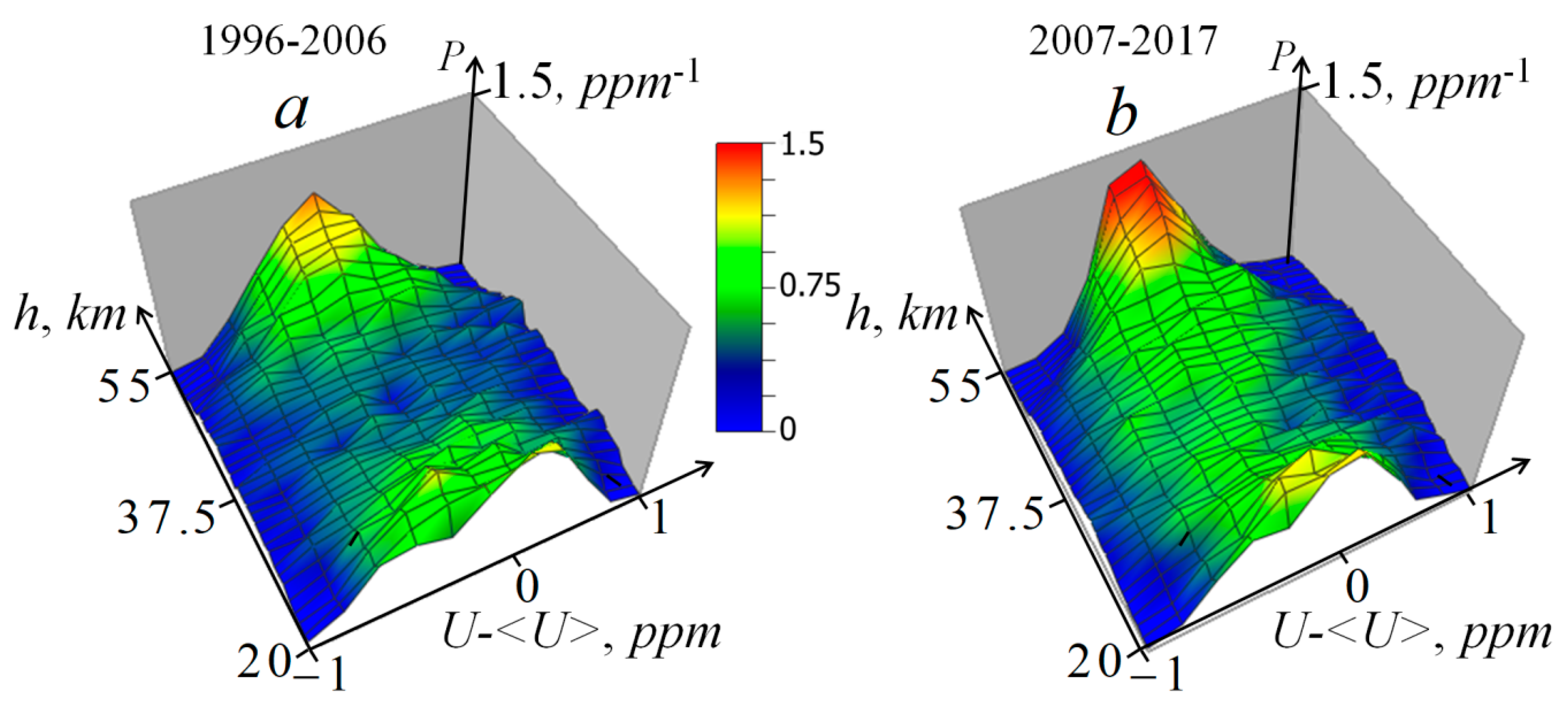
3.3. Probability Distributions of Ozone Variations in Two Decades (1996–2006 and 2007–2017)

In Figure 3, two decade ensembles of ozone profiles are demonstrated.

It is possible to see, in Figure 3, strong variations of ozone profiles in the stratosphere over Moscow that include random and seasonal components. One can mention that profiles for the 2007–2017 decade (Figure 3b) look in some places somewhat broadened and decreased at altitudes of their maxima.

In Figure 4, one can compare distributions of the probability density of variations (deviations from the mean profiles U(h) – <U(h)>) calculated for these two ensembles.

As it is possible to see, in Figure 4, that probability distributions mostly have Gaussian-like shapes, and the probability density is much more widely distributed at altitudes of ozone profile maxima and more localized at lower and higher altitude levels. Additionally, there is a significant difference between results for these two ensembles—variations of 1996–2006 years are more widely distributed than those of 2007–2017, which leads to the significant decrease in mean-square variations in the 2007–2017 decade when compared to those in the decade 1996–2006. Based on the following statistical analysis, seasonal and decade changes of middle-latitude stratospheric ozone will be revealed more clearly.

Below, we demonstrate long-term changes in other statistical parameters, where, taking into account ozone seasonal variations, we began with statistical analysis for separate months. For this, nine separate sub-ensembles for every month of autumn, winter, and spring seasons were extracted from these two decade ensembles.

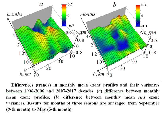
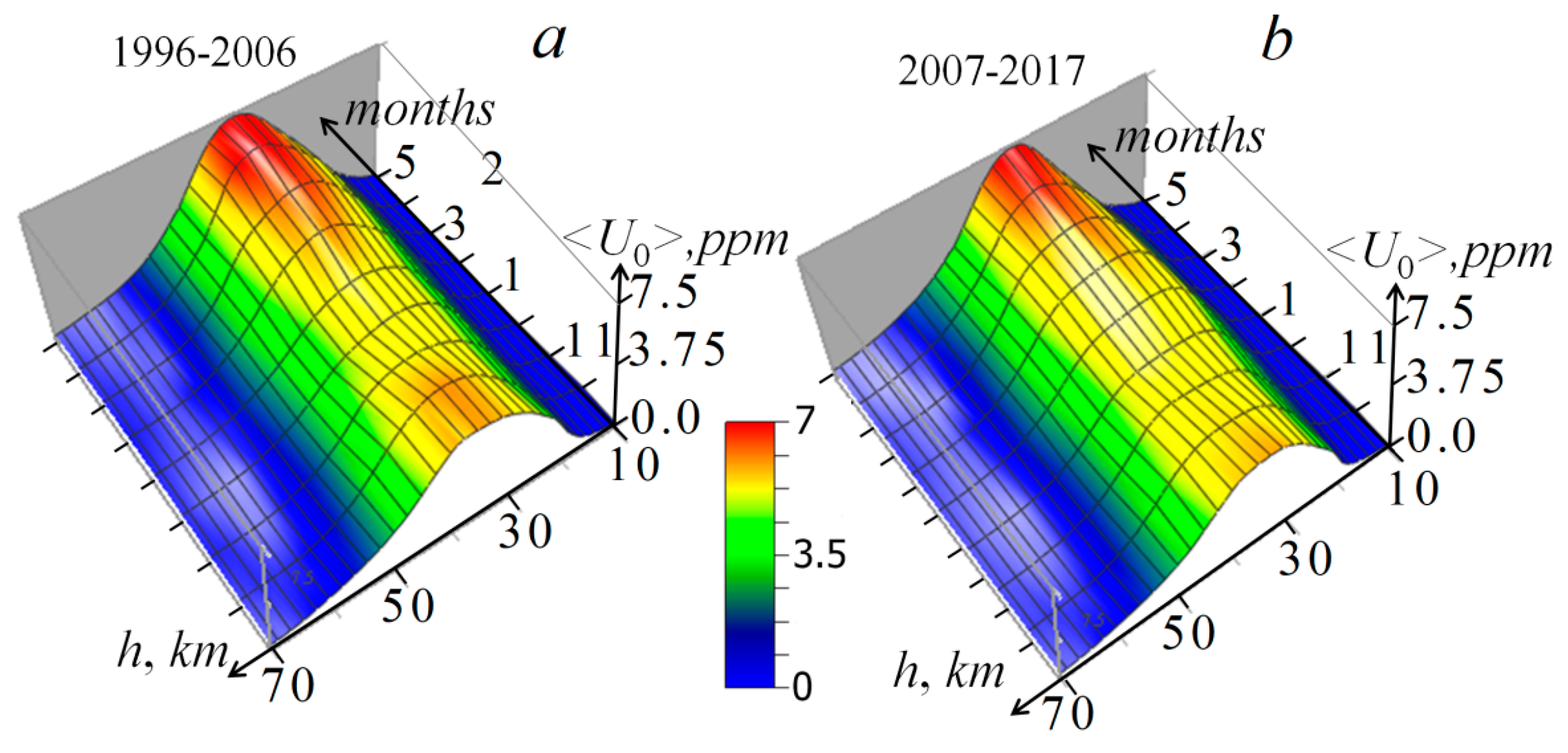
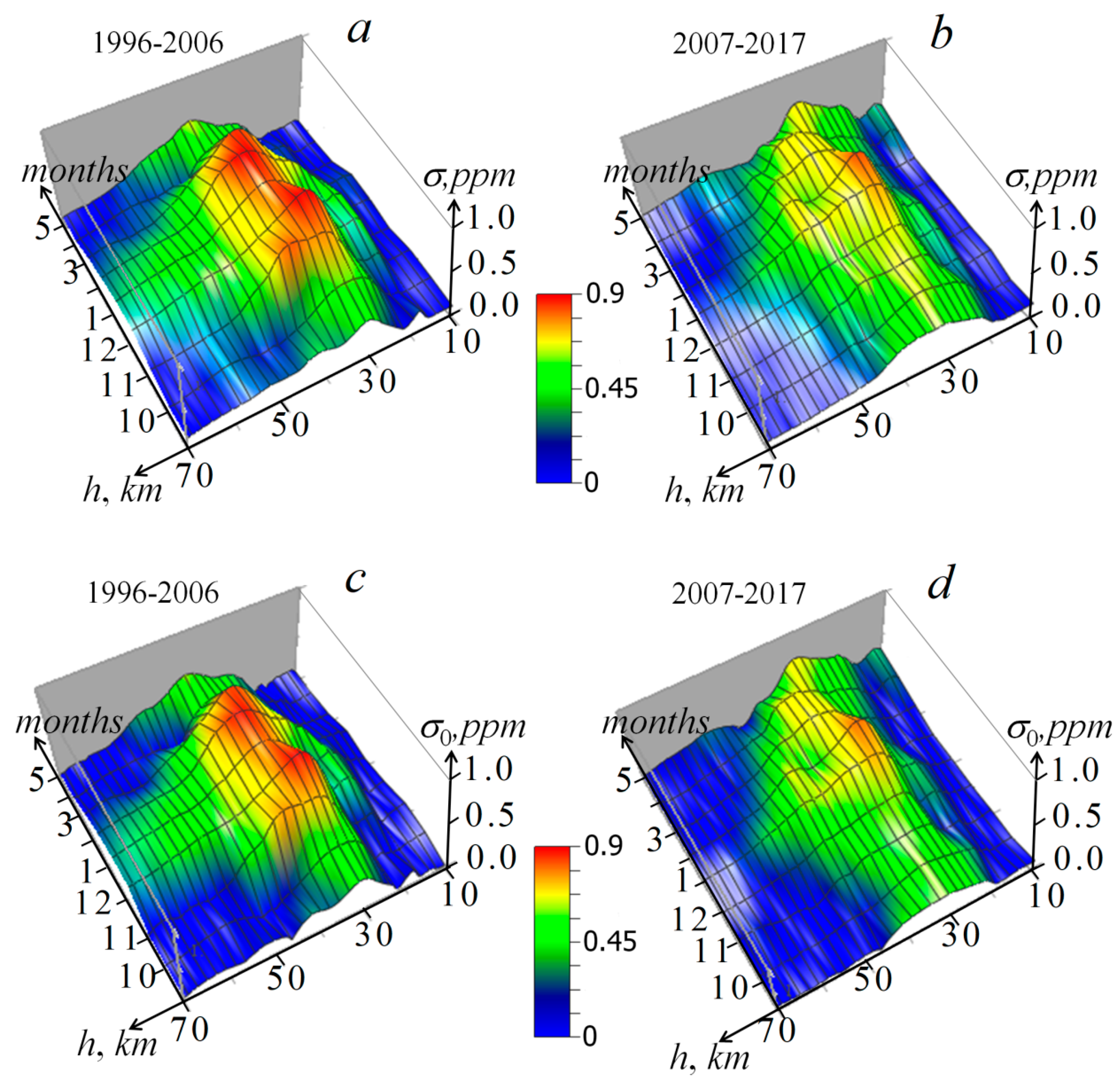
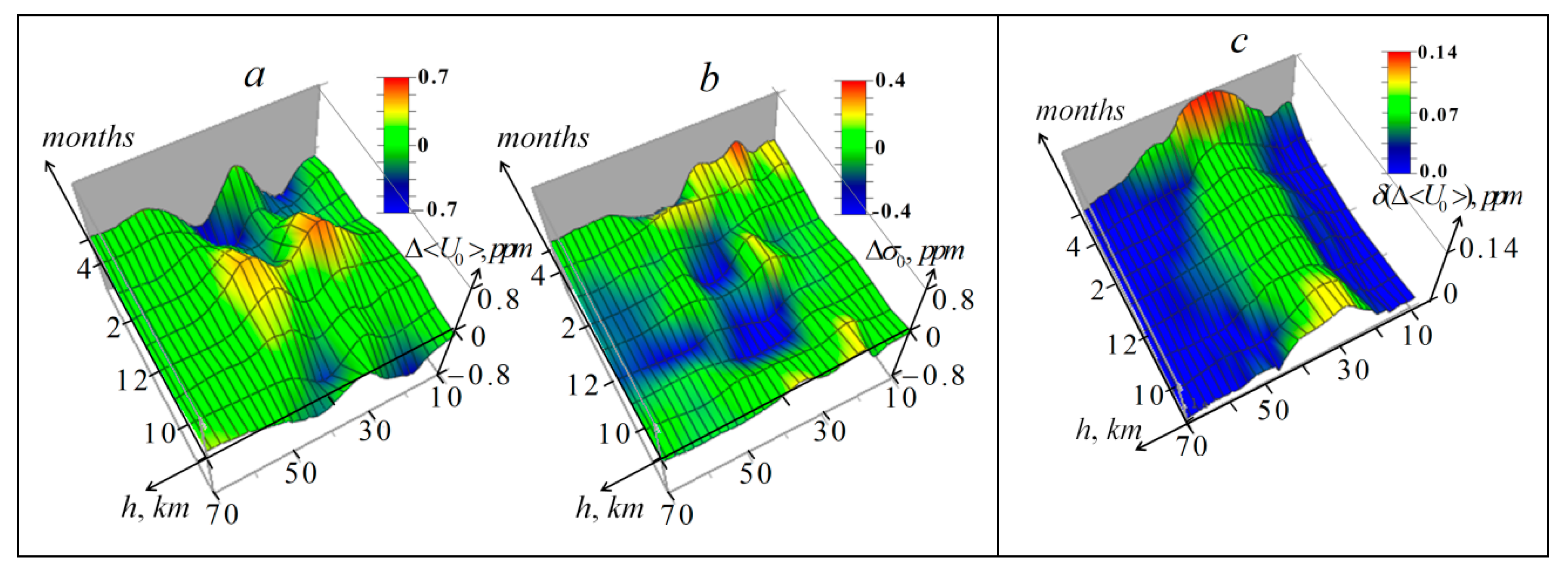
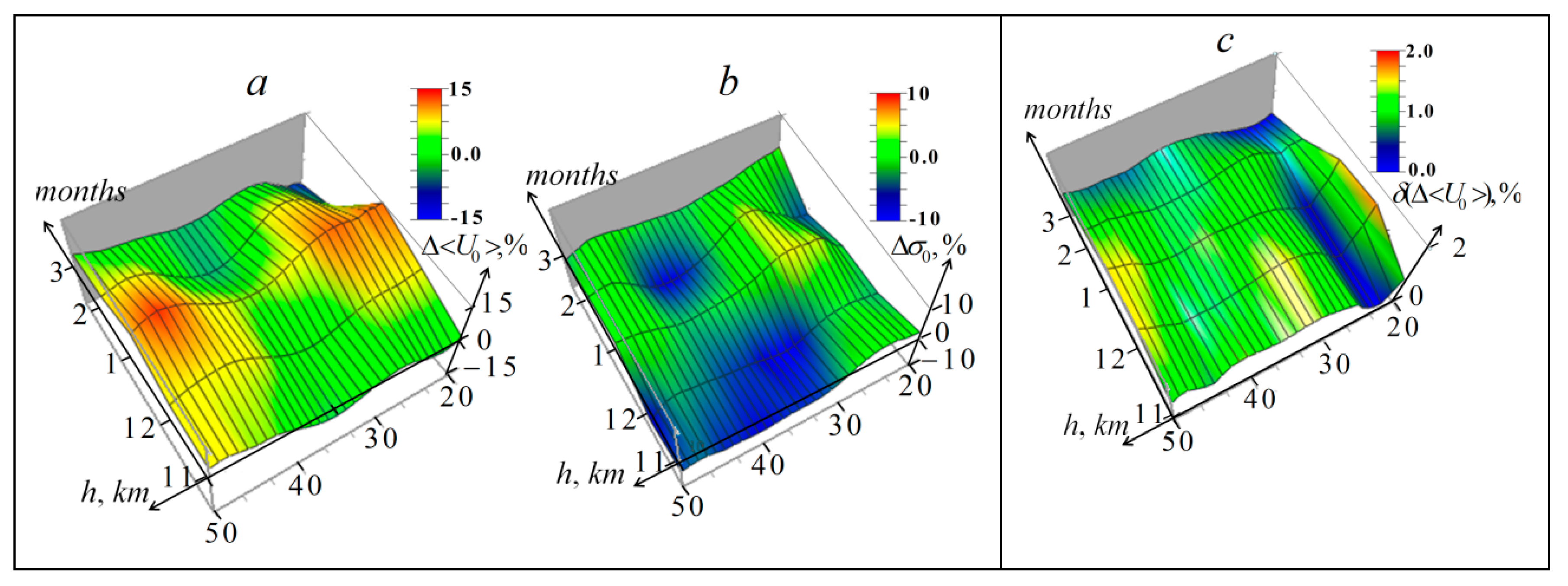
3.4. Mean and Variances of Retrieved Ozone Profiles in Separate Months of Two Decades (1996–2006 and 2007–2017)

In Figure 5, seasonal dynamics of the monthly mean ozone profiles $<U_0(h)>=\frac{1}{M}{\displaystyle \sum _{i=1}^M{U}_{0i}}$ for months from September to May for the 1996–2006 and 2007–2017 decades are given (M is the number of ozone profiles in the corresponding month ensemble that includes profiles obtained in all days of measurements in this month in all eleven years of each of the two decades).

The results shown in Figure 5 demonstrate noticeable seasonal variations of mean ozone profiles that are quite similar for both decades; however, it is possible to discern a decrease in maxima and a wider altitude distribution in cold months (from November to March) of the 2007–2017 decade that are seen much more clearly than in Figure 3. In the decade 1996–2006, the ozone VMR achieved its maximum value of 7.37 ppm at the altitude of 36 km in April; the minimum value (at the altitude of the maximum of the ozone profile) of 5.27 ppm was observed in December at 34 km—so, the maximum seasonal variation amounted to 2.1 ppm (28.5% of the maximum value). In 2007–2017, the same values were 7.29 ppm at 34 km in May and 5.22 ppm at 34 km in December with almost the same difference of about 2.1 ppm (28.4%).

In Figure 6, seasonal dynamics of monthly mean rms variances of retrieved ozone profiles averaged over eleven years of the 1996–2006 and 2007–2017 decades $\sigma =\sqrt{\frac{1}{M-1}{\displaystyle \sum _{i=1}^M{(U_i-<U>)}^2}}$(where M is the same as defined for monthly means in Figure 5) and variances of ozone profiles ${\sigma }_0$ cleared from retrieval errors are demonstrated.

As clearly seen in Figure 6, in the distributions of both retrieved (a, b) and cleared from error (c, d) parameters, ozone variances in the second decade (2007–2017) are essentially decreased as compared to the decade 1996–2006, especially in cold months, which confirms the results shown in Figure 4. It is also interesting to mention two maxima of variability at altitudes higher and lower than corresponding maxima of the ozone profile in the distribution of variances in the winter months of the decade 2007–2017. The maximal value of variances ${\sigma }_0$ in the decade 1996–2006 amounts to 0.92 ppm at 32 km in December; in the decade 2007–2017, it was 0.83 ppm at 30 km in February—both about 12% of the corresponding maximal mean values.

In Figure 7, one can see differences $\mathsf{\Delta }<U_0>=<U_0{>}_{2007-2017}-<U_0{>}_{1996-2006}$ and $\mathsf{\Delta }{\sigma }_0={\sigma }_{02007-2017}-{\sigma }_{01996-2006}$—between ozone parameters shown in Figure 5 and Figure 6 and the distribution of rms sampling errors $\delta (\mathsf{\Delta }<U_0>)=\sqrt{({\sigma }_{\delta U1996-2006}^2+{\sigma }_{\delta U2007-2017}^2}$. Sampling errors of covariance matrixes B and B₂ are independent, so their effect is included at the correction of rms variances demonstrated in Figure 6, and appeared to be not significant.

Relatively stronger decade changes of the monthly mean ozone content were revealed at altitudes higher and lower than the layer maxima positions in Figure 7a. The maximal positive changes (0.59 ppm at 27 km and 0.52 ppm at 44 km—both 12.6% of the mean values in Figure 5a) took place in January, whereas maximal negative changes were registered in September (−0.47 ppm at 19 km—32%), October (−0.39 ppm at 37 km—6.2%), and May (−0.45 ppm at 42 km—8.4% and −0.50 ppm at 19–22 km—26–18%). Corresponding sampling errors shown in Figure 7c are small enough to demonstrate the significance of the revealed changes. It is also seen that these errors are relatively small for cold months (because of the larger number of profiles in ensembles), and corresponding parameters are yet more statistically significant. It is also interesting to mention that the two-maximum structure of changes in January (Figure 7a) on the whole remain in other months, gradually changing in amplitude and shifting to different altitudes in both directions from this month.

In Figure 7b, we see that variability of the ozone layer over Moscow in the 2007–2017 decade was mostly decreased in comparison with 2006–2016, especially in cold months. Maximal strong decreases in the rms variances were detected at altitudes near the ozone profile maximum (−0.35 ppm at 33 km in December and at 39 km in February—decreases of 38 and 46% of the monthly mean variances in 1996–2006, respectively). The revealed noticeable decrease in the ozone layer variability in the middle stratosphere can be considered as the most important and unexpected result of this analysis.

For a better understanding, in Figure 8, relative differences $\mathsf{\Delta }<U_0>,\%=100(<U_0{>}_{2007-2017}-<U_0{>}_{1996-2006})/<U_0{>}_{1996-2006}$, $\mathsf{\Delta }{\sigma }_0,\%=100({\sigma }_{02007-2017}-{\sigma }_{01996-2006})/<U{>}_{1996-2006}$, and distribution of relative rms sampling errors $\delta (\mathsf{\Delta }<U_0>),\%=100\sqrt{({\sigma }_{\delta U1996-2006}^2+{\sigma }_{\delta U2007-2017}^2}/<U_0{>}_{1996-2006}$ are given only for the cold months (from November to March) and in a narrower range of altitudes around the ozone maximum.

In Figure 8, one can see that the general shape of relative changes in monthly mean ozone profiles (Figure 8a) and variances (Figure 8b) is similar: they have two maxima at altitudes higher and lower than the ozone layer maximum (most noticeable in January) and minima at altitudes of the ozone layer maximum. Decade changes in the variances within the region shown in Figure 8 are comparable to changes in the mean profiles: changes of variances span the interval from −7 to 3% (mainly in the negative region), whereas the mean profiles change rather symmetrically from −9 to 14%. The level of sampling errors demonstrated in Figure 8c spans values from 0.8 to 1.9% that confirm statistical significance of the revealed unexpectedly strong offsets.

Below, we demonstrate seasonal features and changes of correlation parameters for each month averaged over years of each of the two decades.

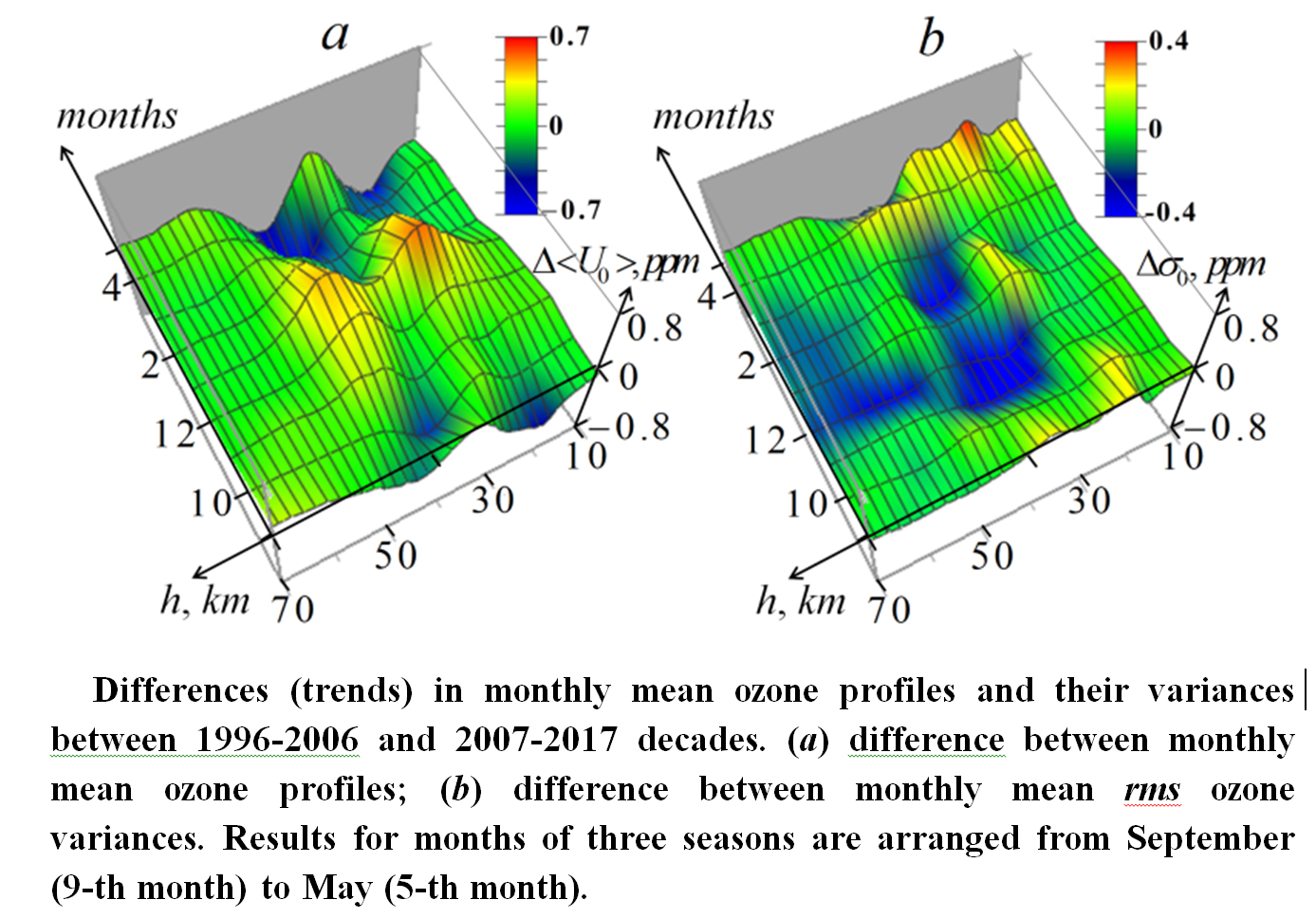
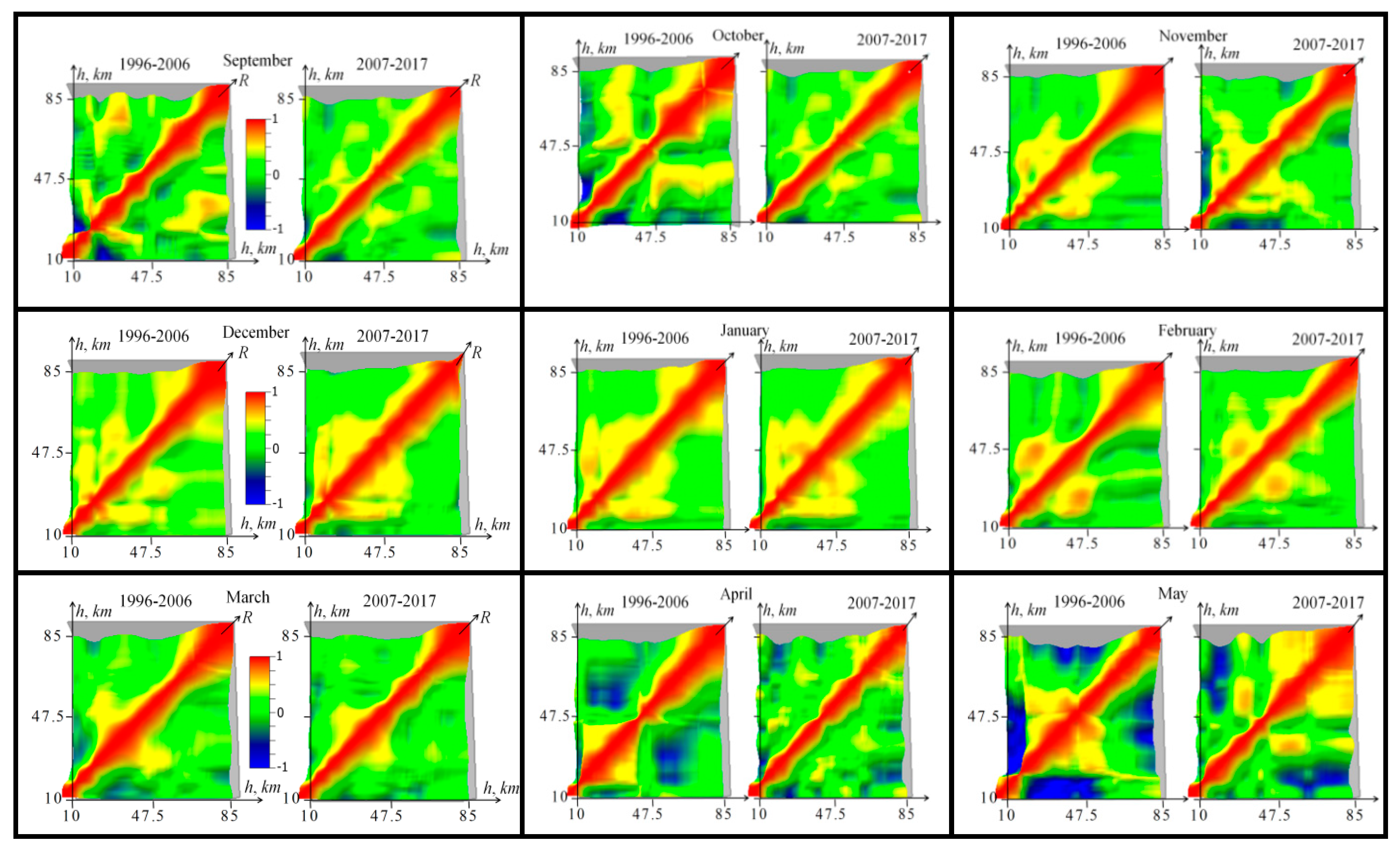
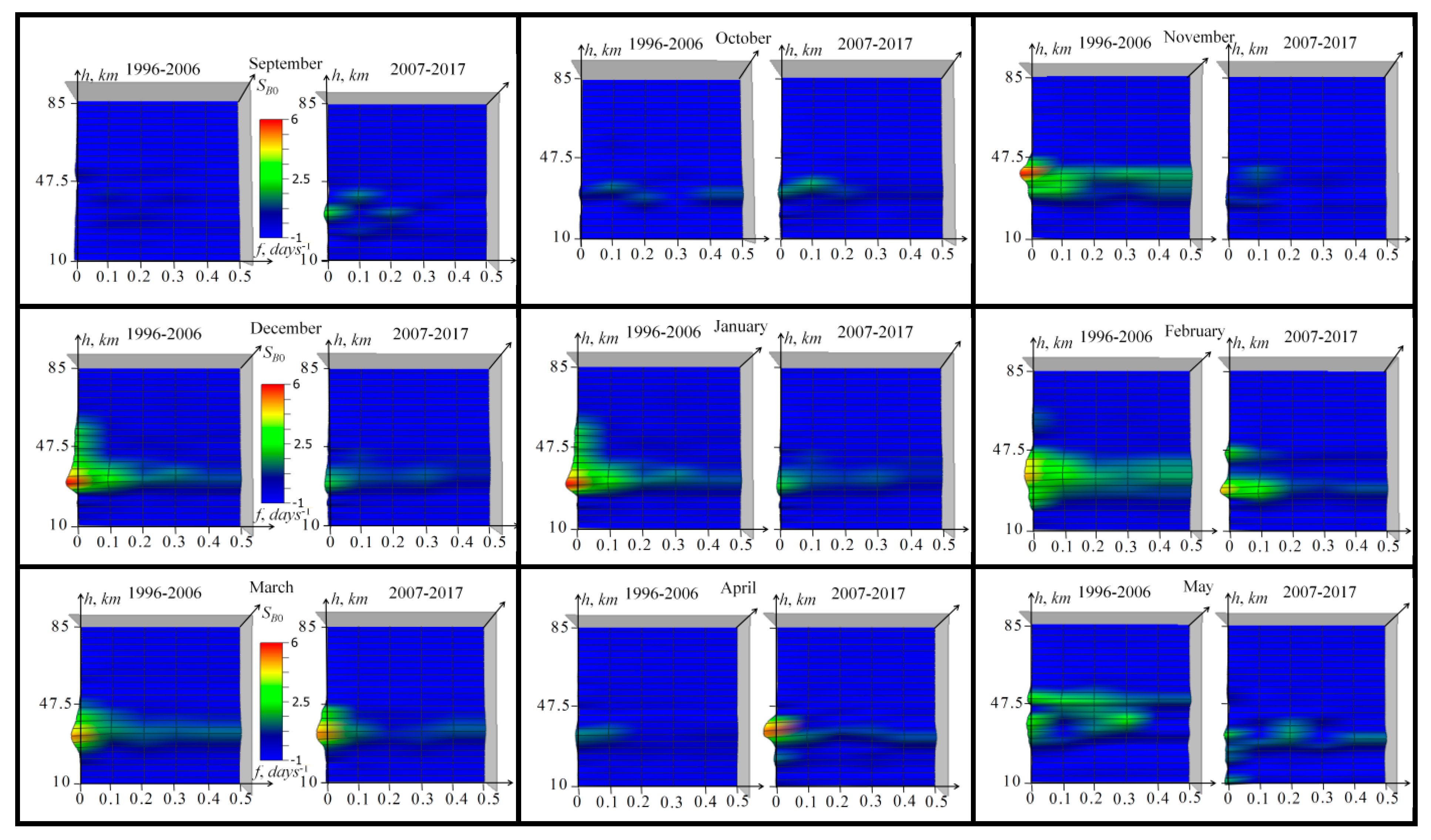
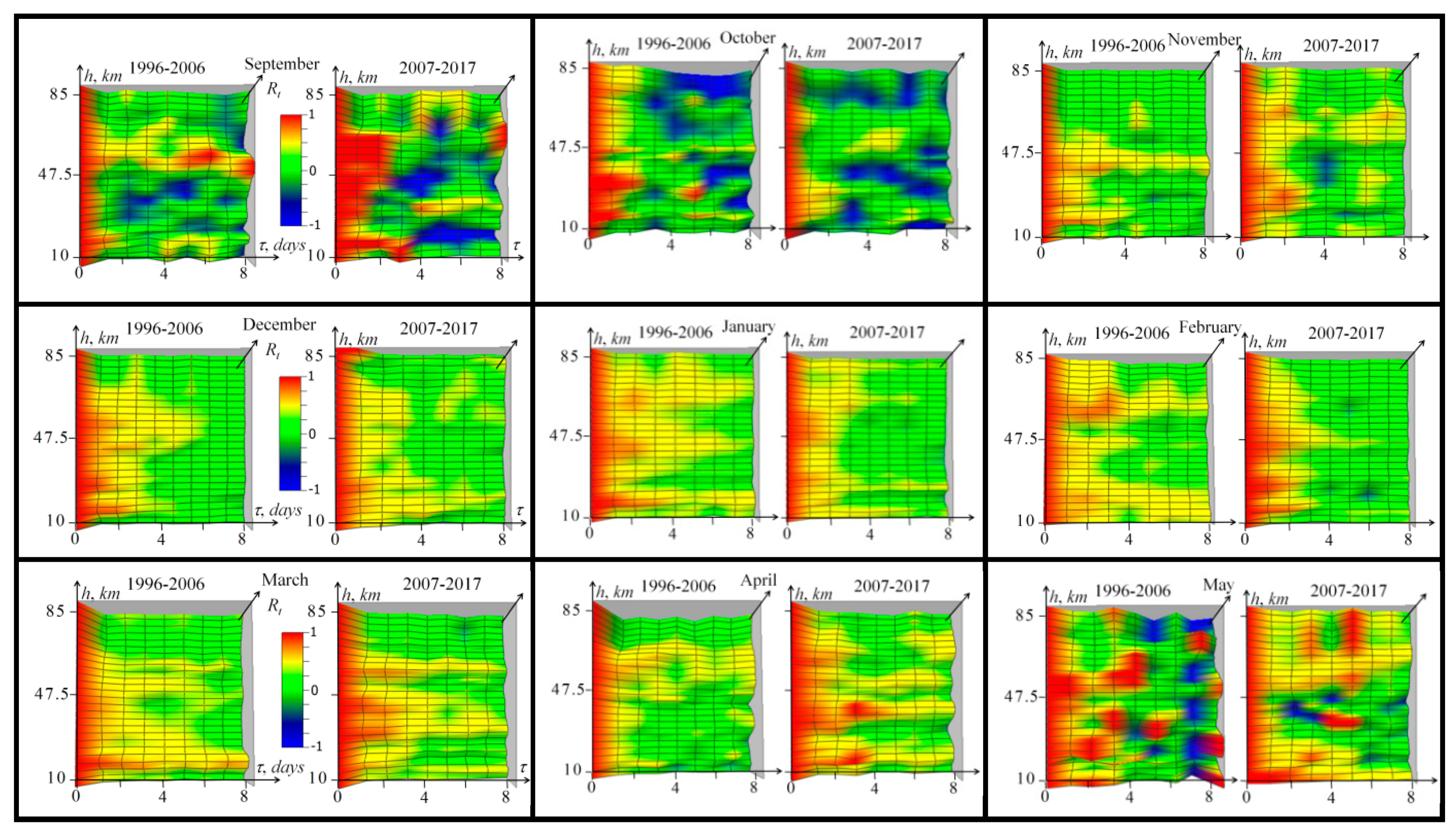
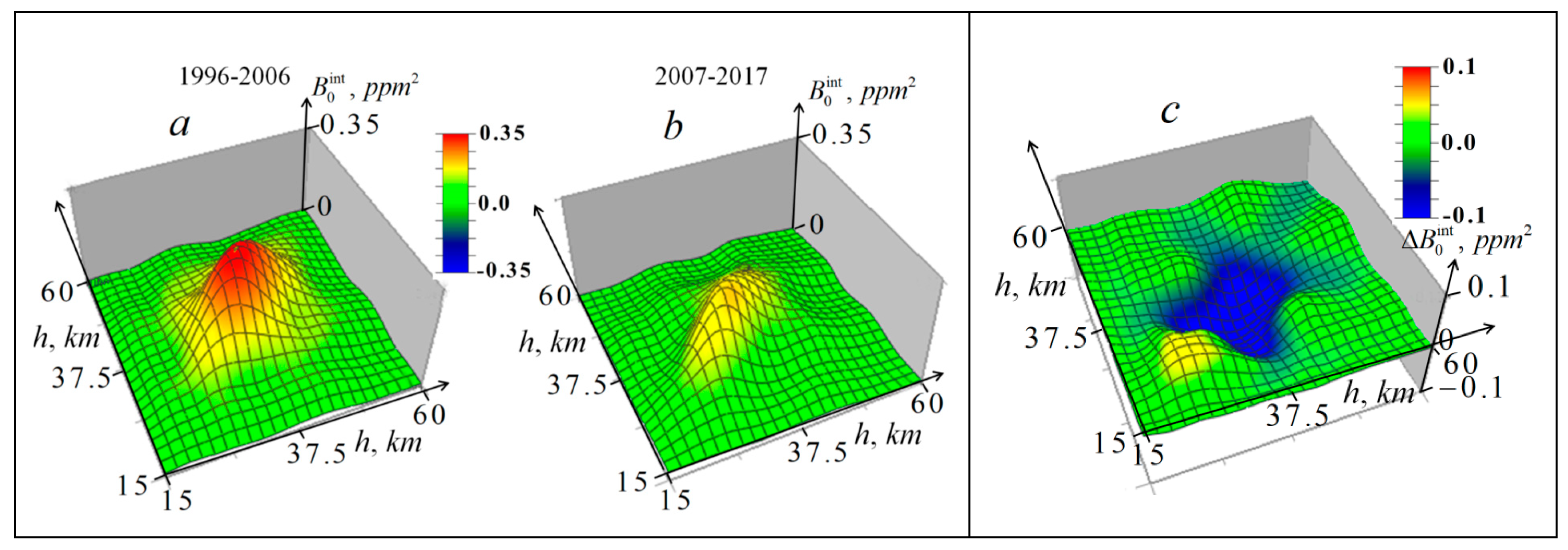
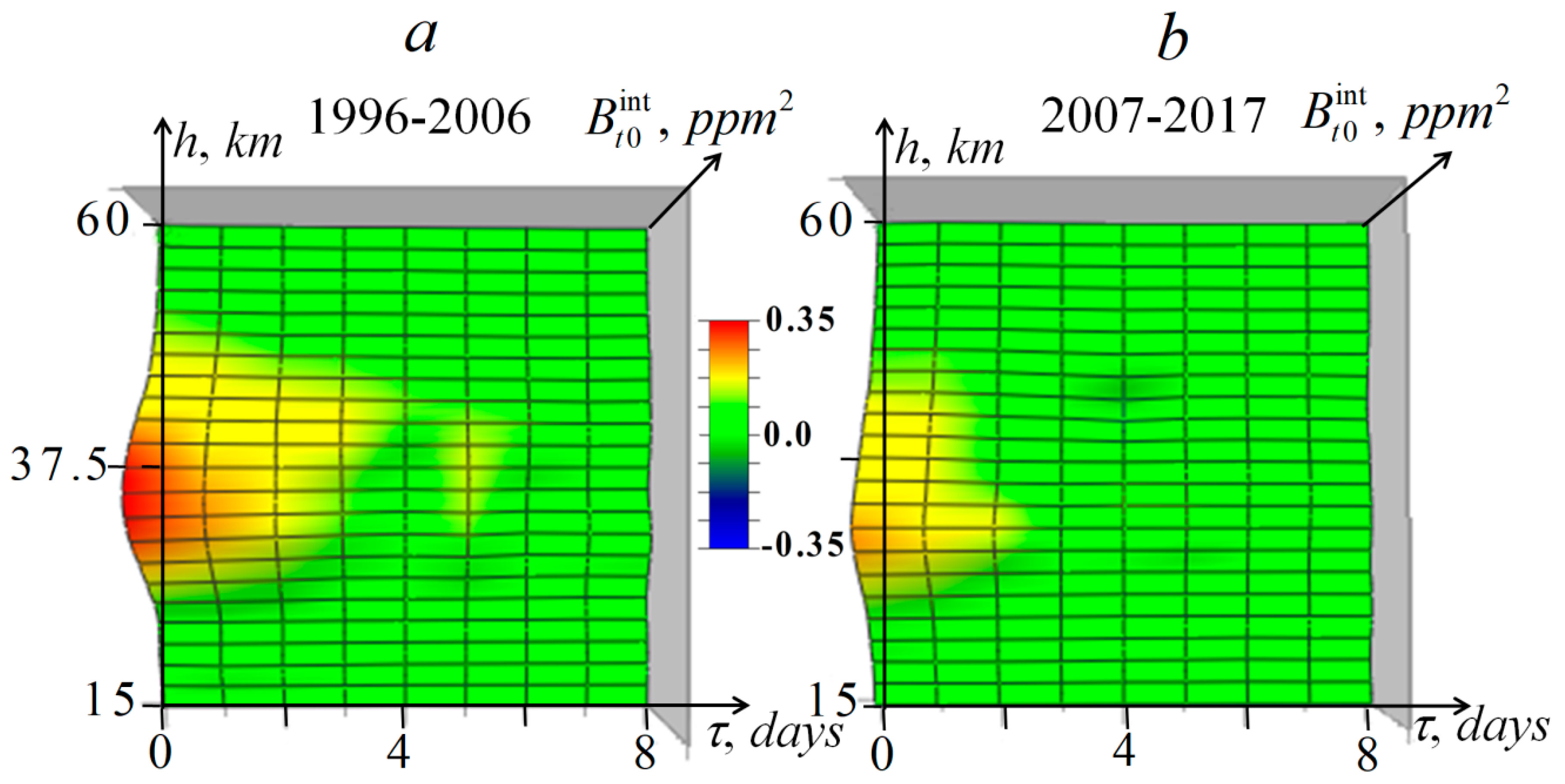
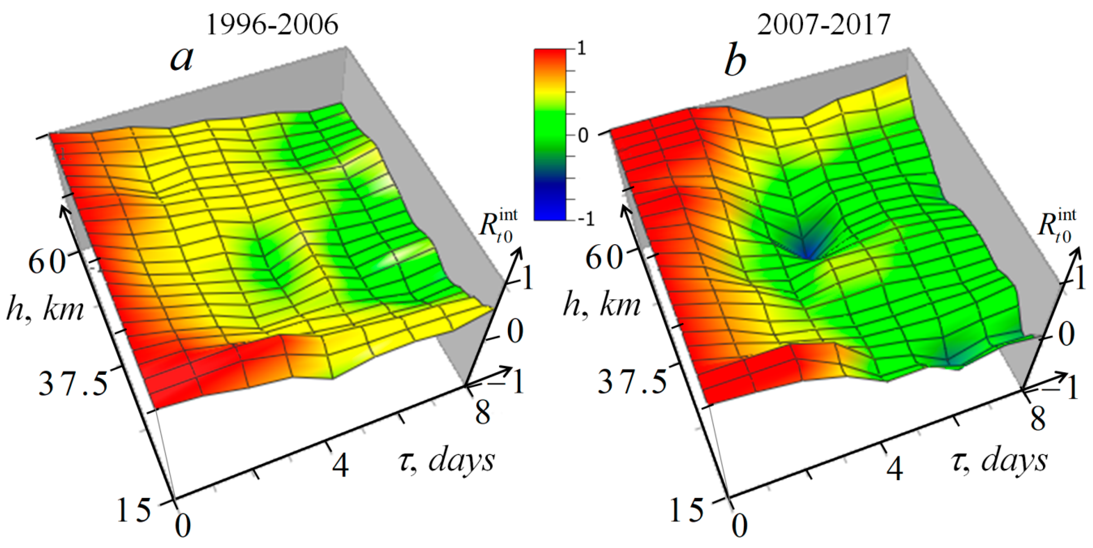
3.5. Inter-altitude and Time Covariance and Correlation Functions in Separate Months of Two Decades (1996–2006 and 2007–2017); Frequency Spectra of Time Covariance and Correlation Functions

In Figure 9, inter-altitude covariance functions cleared from retrieval errors are demonstrated.

Results shown in Figure 9 demonstrate a large seasonal diversity and significant decade changes of inter-level covariance relations that can be interesting for studies of the atmosphere long-term dynamics. The variability of the ozone layer was considerably decreased in the cold months (from November to March) of the decade of 2007–2017 if compared to that in the 1996–2006 decade, whereas it remained unchanged or somewhat increased in near-summer months.

Corresponding inter-altitude correlation features are demonstrated in Figure 10, where noncleared correlation functions R for retrieved ozone profiles are shown (because the cleared correlation functions R₀ have strong distortions in regions of small variances).

One can see here a seasonal diversity and decade changes of inter-level relations, though, on the whole, inter-altitude correlation is unexpectedly stable. Additionally, in most cases, it is worth mentioning that the broadening of high-correlation ranges above altitudes 50–60 km is related to a decrease in sensitivity and resolution of the microwave method with altitude.

In Figure 11, the time covariance functions are given depending on the time shift τ, where more strong seasonal diversity and decade changes are seen.

The results also demonstrate that the seasonal ozone variability is decreased in cold months of the decade 2007–2017 when in comparison with that in the 1996–2006 decade, whereas it increased in near-summer months. Furthermore, in these months, secondary maxima are observed that can be related to some periodical nonstationarity. It is important to mention that random errors of various origin (including those related to errors in the temperature profile) are independent at τ > 0, and, hence, they are efficiently suppressed when averaging, whereas systematic errors are eliminated in time covariance functions. This leads to the much higher statistical significance of these statistical parameters.

The seasonal and decade changes presented in Figure 11 manifested themselves in frequency spectra of time covariance functions given in Figure 12 for the frequency band from 0 up to 0.5 days⁻¹ (the Niquist frequency).

It is seen that spectra for cold moths represent the decrease in the ozone profile variability in the 2007–2017 decade. Secondary maxima observed in some months can be related to periodic processes.

In Figure 13, corresponding time correlation (autocorrelation) functions are demonstrated.

In Figure 13, it is possible to see that distributions of correlation functions sharply decrease with time shift and are very different for cold and near-summer months. For cold months, they monotonously decrease for both decades, but it is seen that for the decade 2007–2017, the correlation time mainly increases, especially in some altitude ranges, which is a clear manifestation of the decrease in the ozone variability in corresponding layers. For summer months, a strong diversity is seen, and the time correlations are quite different from cold months: there are multiple second maxima and minima with a negative correlation that can result from nonstationarity related to large-scale dynamical processes in the stratosphere and propagation of planetary waves or other periodical processes. The typical time of ozone correlation function in Figure 13 is 1–3 days; however, in the above-mentioned cases, more long-term correlations remain of up to 8 days and more.

The frequency spectra of the correlation functions in Figure 13 are given in Figure 14.

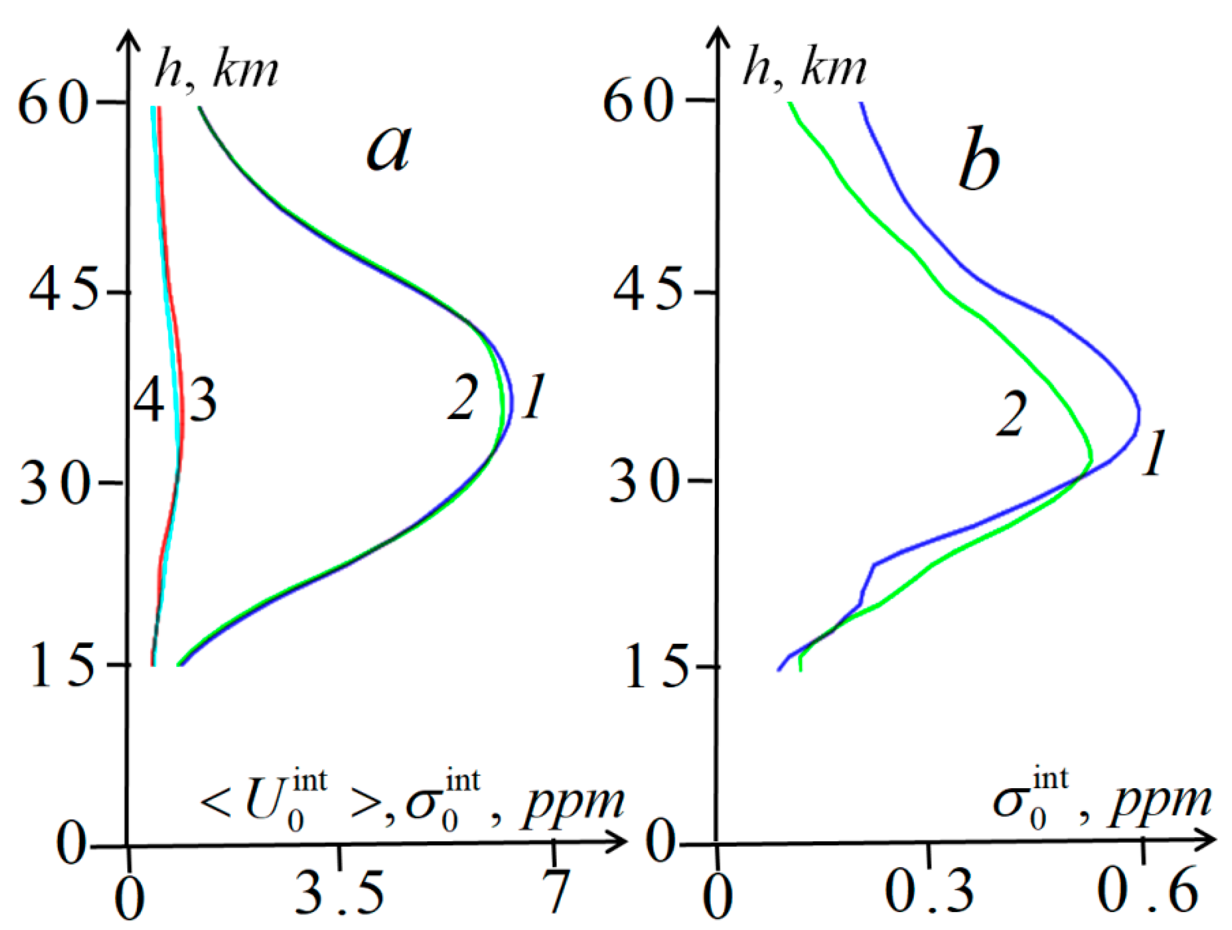
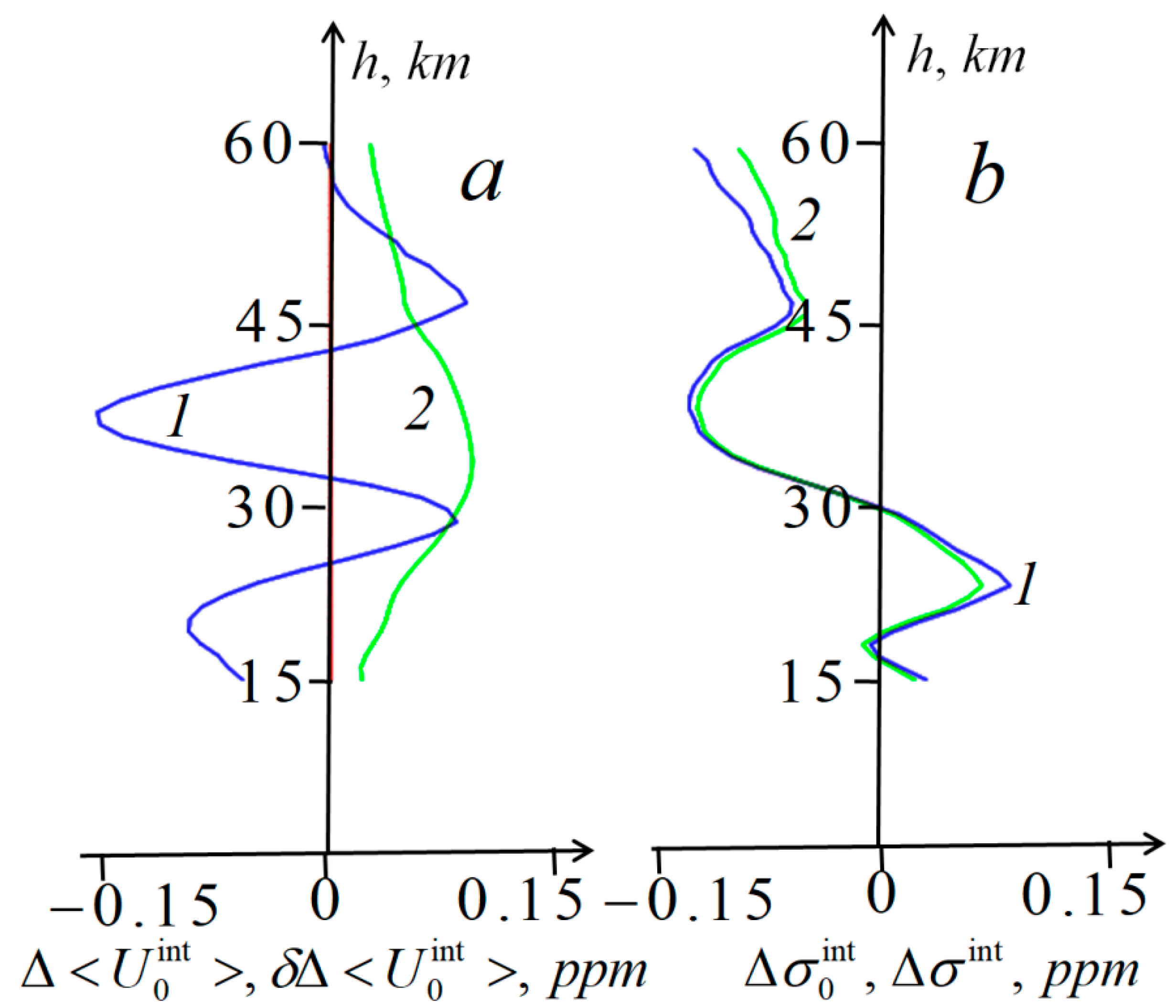
3.6. Integral Statistical Parameters of Ozone Profiles of Two Decades (1996–2006 and 2007–2017).

It is also interesting to average the monthly mean statistical parameters over all the months from September to May to compare seasonally-independent integral parameters for 1996–2006 and 2007–2017 decades. It is possible to reveal some general features of decade ozone offsets using averaged monthly mean (integral mean) parameters:

$<U_0^{\mathrm{int}}(h)>=\frac{1}{M}{\displaystyle \sum _{i=9}^5<U_{0i}>}$,${\sigma }^{\mathrm{int}}(h)=\sqrt{\frac{1}{M}{\displaystyle \sum _{i=9}^5{\sigma }_i^2}}$,${\sigma }_0^{\mathrm{int}}(h)=\sqrt{\frac{1}{M}{\displaystyle \sum _{i=9}^5{\sigma }_{0i}^2}}$,${\sigma }_{\delta U}^{\mathrm{int}}(h)=\sqrt{\frac{1}{M}{\displaystyle \sum _{i=9}^5{\sigma }_{\delta Ui}^2}}$$\mathsf{\Delta }<U_0^{\mathrm{int}}(h)>=<U_{02007-2017}^{\mathrm{int}}(h)>-<U_{01996-2006}^{\mathrm{int}}(h)>$,$\mathsf{\Delta }{\sigma }_0^{\mathrm{int}}(h)={\sigma }_{02007-2017}^{\mathrm{int}}(h)-{\sigma }_{01996-2006}^{\mathrm{int}}(h)$, $\mathsf{\Delta }{\sigma }_0^{\mathrm{int}}(h)={\sigma }_{2007-2017}^{\mathrm{int}}(h)-{\sigma }_{1996-2006}^{\mathrm{int}}(h)$, and corresponding errors of the difference of integral mean ozone profiles $\delta \mathsf{\Delta }<U_0^{\mathrm{int}}(h)>=\sqrt{{[{\sigma }_{\delta U1996-2006}^{\mathrm{int}}(h)]}^2+{[{\sigma }_{\delta U2007-2017}^{\mathrm{int}}(h)]}^2}$, where averaging is carried out over M = 9 months from September (i = 9) to May (i = 5); i is the month number.

In Figure 15a, averaged monthly mean ozone profiles and their averaged variances are shown.

One can see that strong differences in monthly mean profiles between two decades (see Figure 6 and Figure 7) are considerably smoothed in the integral mean decade profiles so that only a small decrease in the maximum can be discerned clearly, whereas it is difficult to discern two maxima at higher and lower altitudes. The smoothing of the changes in the integral mean profile and variances averaged over nine months is related to the seasonal diversity in altitude distributions of monthly mean decade changes (Figure 7).

Changes of the integral ozone profile variances are clearly seen in Figure 15b; a decrease at h > 30 km and an increase at h < 30 km remain rather significant. Together with the revealed decade changes in monthly mean variances (see Figure 6 and Figure 7) this should be considered as the most important result of this research.

In Figure 16, the decade differences between the integral parameters shown in Figure 15 are given.

In this figure, it is more clearly seen that strong changes in monthly mean profiles for separate months between two decades (see Figure 6 and Figure 7) are considerably smoothed in integral mean ozone differences. Moreover, sampling errors of these changes are somewhat increased because they include the deposition of seasonal variations. The decade integral mean ozone changes have the altitude distribution similar to that in the monthly mean changes for winter months (see Figure 7a): decreases by 5.7% at the altitude of 19 km and by 2.6% at 37 km with sampling errors by 1.5%; increases by 1.7% at 28 km and 2.5% at 47 km with errors of 1.6%. The corresponding decade averaged mean column (integral) ozone content above 20 km remained practically unchanged: 4.61 g/m² for the decade 1996–2006 versus 4.58g/m² for 2007–2017.

Changes of the integral mean variances shown in Figure 16b both for cleared and non-cleared variances are comparable to those of monthly mean variances (see Figure 7b) and demonstrate the deep decrease at altitudes above 30 km with the maximum at 38 km (−25% of the value of integral variances for 1996–2006 at this altitude, shown in Figure 15b) and an increase at altitudes below 30 km with the maximum at 23 km (35%). As seen in Figure 16b, these changes are quite similar for cleared and noncleared variances; here, it is noteworthy that absolute values of the latter offsets are somewhat less than those of the cleared one. Sampling errors in the cleared integral variances can be related only to errors of the clearing method, which are, in fact, unknown. However, they obviously cannot exceed the correction itself—i.e., they are for certain less than the difference between cleared and noncleared changes in Figure 16b. Even if one considers this difference as the standard deviation (sigma) of methodic errors, the significance of the revealed variances greatly exceeds the three-sigma criterion.

The similar changes of the ozonosphere were discovered for integral inter-altitude covariance functions. In Figure 17, the cleared covariance functions for two decade integral ensembles are shown together with their difference.

In Figure 17, one can see that the inter-altitude integral mean covariance functions also have drastic changes: the distribution of the covariance functions for 2007–2017 is strongly decreased at altitudes 30–45 km. In these functions for 2007–2017, one can also see secondary maxima. The corresponding regions of positive and strong negative changes are more clearly shown in Figure 17c, where the difference of the covariance functions is provided.

In Figure 18, noncleared inter-altitude integral mean correlation functions for the decade ensembles are shown. It is seen that unlike the integral covariance function shown in Figure 17, integral correlation functions are practically unchanged: only a small decrease in correlation can be discerned at altitudes of the ozone layer maximum for the 2007–2017 ensemble.

It is noteworthy that several times in the decade 2007–2017, the stratospheric polar vortex was inclined so that the lower and middle stratosphere over Moscow was inside the vortex, while the upper stratosphere (40 km and higher) was outside the vortex. The cases resulted in different correlations of ozone concentration with physical parameters of the stratosphere (temperature, potential vorticity) and, correspondingly, in lower inter-level correlations. This could contribute to the small decrease in integral mean inter-level correlation for the decade 2007–2017 seen in Figure 18.

In Figure 19, integral mean time-covariance functions of ozone profiles cleared from the retrieval errors are given.

Comparing results for the two decade ensembles, we can conclude that, like in the case of integral inter-altitude covariance function shown in Figure 17, there is a strong decade change revealed in the decrease in integral mean time-covariance functions at altitudes of 27–47 km. Additionally, it is possible to discern small second maxima of the functions at τ = 5 days seen for both ensembles at altitudes near the ozone layer maximum.

Here, we stress again that the time-correlation parameters are obtained from much more independent (because of time shifts) data, and, hence, they are more reliable and statistically significant. Furthermore, because of this reason, it appeared possible to avoid strong distortions in the cleared time-correlation functions presented in Figure 20.

It is seen in Figure 20 that the inter-altitude correlation functions for the decade 1996–2006, like the corresponding monthly mean correlation functions in Figure 13, have a shorter typical correlation time than those for the 2007–2017 decade, which means a decrease in the variability. Additionally, it is possible to the see the second maximum of functions at τ = 5 days at altitudes near the ozone layer maximum with the deep negative minimum at τ = 4 days that can be related to some long-remained nonstationarity.

3.7. Comparison of Results with Other Research

In the last two decades, many long-term measurements of composition and physical parameters of the middle atmosphere have been carried out using both ground-based and satellite-borne instruments. Among them, results of our research are especially important because its beginning in 1996 practically coincided with the beginning of the ozone recovery since 1997 reported in the most recent and comprehensive review [24]. As noted in [24], since 1997, in the middle and high latitudes, the increase in the total ozone column was small (about 1% per decade) with large inter-annual variations of about 5%. Results of our 22-year study show that the decade offset of integral mean ozone content above 20 km was insignificant and negative—about −0.7%.

As for changes in the ozone profile, its trend in 1997–2016 for latitude zone 35–60N was estimated in [24] as 2–3% at a pressure level of 2 mbar (42 km), 1% at 10 mbar (31 km), and −2–0% at 70 mbar (19 km). So, the trend was positive in the upper stratosphere and decreased to zero and small negative values in the lower stratosphere (see Figure 3.21 in [24]).

Since 2005, numerous comparisons of the LPI ozone profiles with profiles obtained by the MLS Aura instrument [25] over Moscow were performed [26,27]. The comparisons showed that in most cases, the LPI profiles coincided with the MLS ones within the experimental errors of the instruments for both the quiet state of the stratosphere and disturbed cases when ozone profiles with two maxima were observed.

The closest to Moscow ground-based mid-altitude station with a long-time set of ozone profiles is Bern (46.57°N, 7.26°E) where regular ozone measurements with the GROMOS microwave radiometer operated at the same frequency of 142.2 GHz were carried out in 1997–2015 [28]. A comparison of data presented in Figure 3 of the paper with analogous data from [28] showed that seasonal variations in Bern were less pronounced than in Moscow. Changes in integral mean ozone profiles obtained in our research (see Figure 15 and Figure 16) correspond qualitatively to the trends [28] in the upper and lower stratosphere but are quite different (sign-changing) in the middle stratosphere at altitudes of 25–40 km. Here, it should be noted that our data covered only nine months of three seasons (from September to May). Furthermore, they are local, and it is known that results are dependent on the geographical position of the observation points, especially in the north part of middle latitudes. For example, at the same latitude 55N, a shift of the stratospheric polar vortex from the North Pole to Europe in cold months produces quite different (opposite) effects on the stratospheric ozone over Moscow and the Pacific Ocean. As a result, local data on the ozone in the stratosphere for cold months may differ from the zonal mean estimates presented in [24]. Probably the main reason for the difference is the lower latitude of Bern (47N versus 56N for Moscow), so not all shifts of the stratospheric polar vortex to Europe in cold months resulted in noticeable ozone decreases, and the vortex edge rarely passed over Bern.

The decade trends for 1997–2015 revealed from the GROMOS data were 3.14 ± 1.71% at 37 km and −3.94 ± 2.73% at 59 km [28]. On the whole, the trend obtained in Bern more or less corresponds to [24] altitudes lower than 45 km, but is quite different from [24] those above this altitude. Our results at these altitudes give −2.6 ± 1.5% at 37 km and –0.5% ± 3.1% at 59 km. The obtained altitude distributions of decade changes are both alternating-sign but rather different (compare Figure 16 in this paper with Figure 9 in [28]). The World Meteorological Organization ([29], Table 2.4) reported the decade ozone increase of 3.9 ± 1.3 at 40 km in the upper stratosphere at northern midlatitudes (35–60°N) over the 2000–2013 period.

4. Discussion

The results presented in this paper were rather unexpected. The large dimensions of statistical ensembles of the ozone profiles extracted from data which were obtained for the nine months from September to May for each of the two decades 1996–2006 and 2007–1017, and the applied method of clearing of the data from methodical errors provided a high enough statistical significance for our main results. The study of monthly mean ozone profiles, their rms variances, inter-altitude covariance and correlation functions, time covariance and correlation functions, and their frequency spectra revealed seasonal and decade changes of these parameters, especially the strong decrease in ozonosphere variability in cold months of 2007–2017 at altitudes above 30 km. Furthermore, we averaged these parameters over all the months. The decade changes of such integral mean ozone profiles appeared smoothed and mostly not sufficiently statistically significant, whereas the averaged parameters of their variances demonstrated the strong decrease in ozonosphere variability above 30 km in the decade 2007–2017.

Our method of the retrieval errors correction based on their statistical analysis in the numerical simulation with ensembles of retrieved profiles enabled us to obtain more reliable results. However, it should be mentioned that it appeared difficult to take into consideration some errors related to calibration, apparatus function, as well as the influence of temperature profile errors on the kernel of the solved integral equation. One can expect that the effect of these sources of the retrieval errors can be compared to that of the signal noise. If so, the corresponding unaccounted correction of the covariance functions can be comparable to that of noise that were taken into account in the results demonstrated in Figure 6 and Figure 16—i.e., rather inessential—especially because some of these unaccounted corrections should be correlated for different days. Consequently, the main results will be practically unchanged—especially bearing in mind that there is no reason to expect some seasonal and decade offsets of these errors. Hence, they could not significantly change the main results. In this paper, time-correlation functions were calculated for monthly mean ozone profiles and for integral mean profiles averaged over the 1996–2006 and 2007–2017 decades.

To avoid the influence of the seasonal unstationarity, they are presented here only at 8-day time intervals, so, we could not reveal in these statistical parameters the influence of the stratospheric ozone variations over Moscow with periods of several weeks typical for planetary waves. These strong variations observed in winter months as a result of shifts of the stratospheric polar vortex poor in ozone air to Europe and back to the North Pole can be discerned in Figure 3. So, as a subject of future research, the study of time correlation periods of 2–8 weeks is planned. For this, it will be necessary to distract at calculations seasonal changes of mean ozone profiles.

To explain revealed changes in both ozone profiles and their variances in the stratosphere over Moscow, it is necessary to take into account that the geographical position of Moscow (56N, 37E) allowed observing alternations of air masses of very different origins, especially in periods of violent stratospheric disturbances and stratospheric warmings.

The main factors influencing the ozone profile and its integral content in the stratosphere (~90% of the total ozone column content) at time scales of weeks and months are stratospheric dynamics (both large-scale and mesoscale) and photochemistry (especially reactions with ozone-depleting substances). Both of the factors are related to each other, seasonally dependent, and vary considerably from year to year. Dynamics is the most important in the lower and middle stratosphere, while the role of photochemical processes increases in the upper stratosphere and mesosphere. To date, predictions of large-scale dynamical events such as planetary waves, stratospheric warmings, and their inter-annual variations are difficult and unreliable. At time scales of years and decades, the stratospheric ozone is additionally influenced by solar activity, quasi-biennial and other atmospheric and oceanic oscillations, trends in ozone-depleting substances content and spatial distribution, aerosol from volcanic eruptions, etc. [30].

The 1996–2017 ozone observations at the LPI occasionally but almost exactly covered the 23red and 24th 11-year solar cycles (see in Figure 21 the corresponding solar activity dynamics according to https://yandex.ru/images/search?text=11-years%20cycle%20of%20solar%20activity&stype=image&lr=47&source=wiz&pos=25&img_url=https%3A%2F%2Fwww.spaceweather.live%2Fimages%2Fnews%2F400-header.jpg&rpt=simage).

Expected variations of column ozone content related to changes in solar activity amount to 1–2% with the maximum in polar latitudes [30]. Solar activity in the 24th cycle was almost twice lower than that in the 23rd one. In the absence of other factors, it should have resulted in a decrease in the mean column ozone content during the 24th cycle in comparison to the 23rd one. In our measurements, the difference between integral mean ozone content above 20 km in the decades 2007–2017 and 1996–2006 was small and negative—about −0.7%. It is most probable that obtained minor differences between the two decades for both the integral mean ozone content above 20 km and integral mean ozone profile (see Figure 15a) resulted from the cumulative effect of solar activity; trends of ozone depleting substances; and changes in global atmospheric dynamics, composition (increase in CO₂ content), and temperature. It should also be mentioned that relative variations of the ozone concentration in the upper stratosphere and lower mesosphere related to solar activity are more significant than those of the corresponding integral ozone content. For example, it is reported that in the 23rd cycle, relative ozone changes between the solar minimum and maximum in the region of the Antarctic ozone hole amounted to 6.8–9.6% at altitudes of 22–31 km [31]. So, this effect could be considered as one of reasons for the decrease in variances in the 2007–2017 decade.

Aerosol influence resulted from Eyjafjallajökull eruption in 2010, and wildfires of the last years were negligible—much smaller than the negative contributions after eruptions of El Chichon in 1982 and Pinatubo in 1991. The effect from the last one almost disappeared in 1996 [30].

To explain noticeable and statistically significant decade offsets of monthly mean ozone profiles and their variances as well as of variances of integral mean ozone profiles (see Figure 4, Figure 5, Figure 6, Figure 7 and Figure 8, Figure 15 and Figure 16), we suppose that these changes are related mostly to long-term changes of large-scale dynamics of the stratosphere. This explanation is based on [32], where the influence of strong sudden stratospheric warmings on the ozone in the middle stratosphere over Moscow was studied for cold seasons (we will call them “winters”) from 1995–1996 to 2014–2015. Analysis of several geophysical parameters at a 10 mbar pressure level (altitude about 30 km) such as amplitudes of planetary waves n = 1 and n = 2, geopotential height in the stratospheric polar vortex center, speed of mean zonal wind at 85°N and 60°N, and difference of mean zonal temperatures at 85 and 60N allowed the winters to be divided into four groups:

Group I—winters with major mid-winter stratospheric warming in January; in December polar vortex was shifted to Europe.

Group Ia—winters similar to those of Group I, but the mid-winter stratospheric warming occurred in February, approximately a month later than in Group I.

Group II—winters without strong mid-winter stratospheric warming; polar vortex was deep and long-living; its center was close to the North Pole.

Group III—winters with the shallow stratospheric polar vortex and minor stratospheric warming in December.

The distribution of winters is illustrated by Figure 22.

Ozone profiles (see Figure 3) were noticeably different for various groups of winters. For Group I, the polar vortex rose rapidly and was often shifted to Europe in November and December, so the zone of low ozone concentration in the vortex typically occurred over Moscow. As a result, ozone mixing ratio fell in December to low values of $u_{\mathrm{I}}$≈ 4.5 ppm at the pressure level 10 mbar [32] (herein, we use values averaged through the group of winters). In January, when mid-winter stratospheric warmings occurred, the vortex deformed and filled with rich in ozone air from anticyclone regions. This resulted in a sharp increase up to $u_{\mathrm{I}}$ ≈ 6–6.5 ppm over Moscow in January and February with subsequent growth up to ~7 ppm in March and April [32].

Otherwise, in winters of Group II, the polar vortex formed a little later and only sometimes was shifted to Europe, so averaged ozone mixing ratio in the stratosphere over Moscow in November and December decreased slower than for Group I; its typical value in December was $u_{\mathrm{II}}$ ≈ 5–5.5 ppm at 10 mbar. This level lasted until the beginning of February, then the ozone concentration grew smoothly up to 6.2–6.7 ppm in March and April. So, in December, the difference $u_{\mathrm{I}}$-$u_{\mathrm{II}}$ was negative and decreased to ≈ −1 ppm. In contrast, in January and at the beginning of February, the difference became positive and reached 1 ppm and above. The resulting span of its variations was typically about 2 ppm [32].

For winters of Group Ia, the variations of ozone concentrations were similar to those of Group I, but transitions from low to high values in the middle stratosphere occurred later, in February. Negative differences of $u_{\mathrm{Ia}}$-$u_{\mathrm{II}}$ lasted longer (in December and January). Correspondingly, positive values of the $u_{\mathrm{Ia}}$-$u_{\mathrm{II}}$ difference after the mid-winter stratospheric warming in February were lower and lasted for a shorter time.

In winters of Group III, the main course of ozone changes in the stratosphere over Moscow was similar to that for winters of Group II with irregular but more or less uniform variations of difference $u_{\mathrm{II}}$-$u_{\mathrm{III}}$ within approximately from −0.6 to 0.8 ppm at 10 mbar level from October to May.

Preliminary estimates of monthly mean ozone variances at 30 km averaged through winters of the four groups showed that the variances increased from minimum to maximum for winters of Groups I, Ia, II, and III. So, the ozone concentrations in winters of Groups II and III were more volatile, mainly because of multiple shifts of the polar vortex to Europe and back to the North Pole. For example, the winter 1996–1997 was the most turbulent one, with 12 shifts of the polar vortex back and forth from November to April. Obvious exceptions from the tendency were January data for winters of Group I and February data for winters of Group Ia—the months when mid-winter stratospheric warmings occurred.

To understand some features of changes in monthly mean ozone profiles and their variances between decades 2007–2017 and 1996–2006 presented in Figure 4, Figure 5, Figure 6, Figure 7 and Figure 8, Figure 15, and Figure 16, we have to compare numbers of data sets with low or high mean ozone concentration values and with low or high variances for the decades. For example, from Figure 22, one can see that for the decade 1996–2006 in January, there are 2 sets from Group I with a high ozone concentration and 1 set from Group Ia with a low concentration in the middle stratosphere. For the decade 2007–2017, the corresponding numbers are 5 and 2. This means that in January, the mean ozone concentration for the decade 2007–2017 was greater than that for the decade 1996–2006. This could be a reason for the highest maximum in Figure 7a for January at altitudes around 30 km for the difference between monthly mean ozone profiles for two decades.

Similarly, it is possible to find reasons for changes of monthly mean variances. Note that low-volatile contributions to monthly mean variances originated from winters of Group I (except for January) and Group Ia (except for February); high-volatile ones came from Groups II and III together with January of Group I and February of Group Ia. Using these simple rules, we obtained that the significant increase in the number of low-volatile months and corresponding decrease in the number of high-volatile months for the decade 2007–2017 in December and February resulted in the appearance of two deep minima at altitudes of 30–40 km in changes of monthly mean variances in Figure 7b. On the other hand, in January for the decade 1996–2006, the numbers of low- and high-volatile contributions were close to those for the decade 2007–2017. This can explain the small difference between variances of monthly mean ozone profiles in the middle stratosphere in January (see Figure 7b).

These simple examples illustrate the influence of differences in distribution of various winters within the decades on results of statistical analysis.

Taking into account preceding discussion, we can also qualitatively explain noticeable changes in the probability density of ozone profile variations between the decades presented in Figure 4. The bimodal character of ozone profile variations related to multiple shifts of the polar vortex to Europe and back to the North Pole was typical for winters of groups II and III, which prevailed in the decade 1996–2006 (see Figure 22). So, in the stratosphere over Moscow, the polar vortex poor in ozone air often alternated with rich in ozone air masses outside the vortex. Some hints to this bimodality with spans of 1–2 ppm are seen in Figure 4a for altitudes of an ozone profile maximum of 30–35 km. Whereas winters of Groups I and Ia prevailing in the decade 2007–2017 (Figure 22) were less volatile, ozone profile variations occurred not so often and their spans were smaller. So, distribution of the probability density of ozone profile variations for the 2007–2017 decade shown in Figure 4b is considerably narrower.

5. Conclusions

In this paper, the results of the statistical analysis of ensembles of the atmospheric ozone volume mixing ratio profiles over Moscow for 1996–2017 are presented. The profiles were obtained from ground-based day-time microwave measurements of thermal emission in the atmospheric ozone spectral line centered at a frequency of 142.175 GHz carried out at the P.N. Lebedev Physical Institute of the Russian Academy of Sciences for the two decades. Ground-based microwave radiometry is low-dependent on weather conditions in comparison with ground-based optical instruments. It allows day-and-night measurements of the ozone profile from the upper troposphere to the lower mesosphere. So, the method is very effective and suitable for long-term monitoring of the atmospheric ozone profile and its changes. The geographical position of Moscow allows air masses of very different origins to be observed, which leads to strong variations of the ozone profile, especially in periods of violent stratospheric disturbances and stratospheric warmings. Because of these reasons, the results obtained in the same place and with the same method for more than twenty years since the recovery of the ozone layer began are very important—especially for the study of long-term changes of the ozone layer. Additionally, the 1996–2017 ozone observations at the LPI almost exactly covered the 23rd and 24th 11-year solar cycles. The important improvement of the ozone data analysis was provided with the use of the proposed method of clearing statistical parameters from the retrieval errors.

Results presented in the paper reveal significant changes in calculated statistical parameters between decades 1996–2006 and 2017–1017 that demonstrate that the evolution of the ozonosphere consists of not only the ozone column change (its decade mean remained practically unchanged) but of multiple seasonal, inter-annual, and more long-term transformations of the ozone profile: strong decade changes in monthly mean variability, altitude distribution of ozone mixing ratio, and space-time correlations.

It was found that relatively stronger decade changes in the monthly mean ozone profiles were observed at altitudes higher and lower than the maximum ozone volume mixing ratio profile. The maximum positive offsets of 13% of the mean value were discovered at 27 and 44 km in January, whereas maximum negative changes amounted to 32% in September and 26% in May at an altitude of 19 km. The main and unexpected result of this research is the drastically decreased variability of the ozonosphere at altitudes above 30 km, especially in cold months—the decrease in dispersion, inter-altitude, and time variations of the ozone profiles. The maximum fall was detected in February for the monthly mean variances at an altitude of 39 km in the decade 2007–2017—46% of those in the decade 1996–2006.

Significant changes were also revealed in distributions of other statistical parameters: probability density of the ozone profile variances, seasonal changes in monthly mean inter-altitude, and time covariance and correlation functions of the ozone profiles—as well as in frequency spectra of these functions.

Furthermore, monthly mean statistical parameters were averaged over all the months from September to May to compare obtained seasonally-independent integral mean parameters for 1996–2006 and 2007–2017 decades. Changes of integral monthly mean ozone profiles appeared considerably smoothed with a small decrease of 2,6% (with sampling error 1.7%) in the profile maximum at 37 km; the maximum became somewhat wider, and its values at lower and higher altitudes were increased by 1.7% at 28 km and 2.5% at 47 km (with sampling errors of 1.7%). Additionally, the integral mean ozone profile decrease amounted to 5.7% at the altitude of 19 km (with 1.8% sampling error). Here, it should be mentioned that the corresponding decade averaged column (integral) ozone content above 20 km remained practically unchanged—4.61 g/m² for the decade 1996–2006 versus 4.58g/m² for 2007–2017.

Integral variance profiles demonstrated the increase at an altitude below 30 km with the maximum at 23 km (35% of the value of variances for 1996–2006 at this altitude) and decrease at altitudes above 30 km with the maximum at 38 km (−25%). These offsets of variances are statistically significant—like the changes observed in inter-altitude and time covariance functions.

It is possible to conclude that strong decade changes in the ozonosphere revealed in the monthly mean ozone profile are mostly smoothed at the averaging over nine months of analysis, whereas they remain statistically significant for parameters of the profile variations, especially the deep decrease in ozonosphere variability above 30 km in the cold months of the 2007–2017 decade. As possible factors of this decrease, the transformation of the stratosphere large-scale dynamics between two decades and the simultaneous large reduction in the solar activity in the 2nd decade are proposed and discussed. Furthermore, the contradiction between the decrease in the ozonosphere variability above 30 km and growth of variability and instability of the atmosphere because of global warming is intriguing and deserves special attention.

References

1. SPARC/IO3C/GAW Report on Long-Term Ozone Trends and Uncertainties in the Stratosphere; SPARC Report No. 9; Petropavlovskikh, I.; Godin-Beekmann, S.; Hubert, D.; Damadeo, R.; Hassler, B.; Sofieva, V. (Eds.) SPARC: Richmond, VA, USA, 2019; Available online: http://www.sparc-climate.org/publications/sparc-reports (accessed on 10 October 2020). [CrossRef]
2. Steinbrecht, W.; Froidevaux, L.; Fuller, R.; Wang, R.; Anderson, J.; Roth, C.; Bourassa, A.E.; Degenstein, D.A.; Damadeo, R.; Jones, N.B.; et al. An update on ozone profile trends for the period 2000 to 2016. Atmos. Chem. Phys. 2017, 17, 10675–10690. [Google Scholar] [CrossRef] [Green Version]
3. Manney, G.L.; Lawrence, Z.D.; Santee, M.L.; Livesey, N.J.; Lambert, A.; Pitts, M.C. Polar processing in a split vortex: Arctic ozone loss in early winter 2012/2013. Atmos. Chem. Phys. 2015, 15, 5381–5403. [Google Scholar] [CrossRef] [Green Version]
4. Tao, M.; Konopka, P.; Ploeger, F.; Grooß, J.-U.; Müller, R.; Volk, C.M.; Walker, K.A.; Riese, M. Impact of the 2009 major sudden stratospheric warming on the composition of the stratosphere. Atmos. Chem. Phys. 2015, 15, 8695–8715. [Google Scholar] [CrossRef] [Green Version]
5. Smyshlyaev, S.P.; Pogorel’tsev, A.I.; Galin, V.Y.; Drobashevskaya, E.A. Influence of wave activity on the composition of the polar stratosphere. Geomagn. Aeron. Engl. Transl. 2016, 56, 95–109. [Google Scholar] [CrossRef]
6. Wang, W.; Tian, W.; Dhomse, S.; Xie, F.; Shu, J.; Austin, J. Stratospheric ozone depletion from future nitrous oxide increases. Atmos. Chem. Phys. 2014, 14, 12967–12982. [Google Scholar] [CrossRef] [Green Version]
7. Manney, G.L.; Santee, M.L.; Rex, M.; Livesey, N.J.; Pitts, M.C.; Veefkind, P.; Nash, E.R.; Wohltmann, I.; Lehmann, R.; Poole, L.R.; et al. Unprecedented Arctic ozone loss in 2011. Nature 2011, 478, 469–475. [Google Scholar] [CrossRef]
8. Kulikov, U.U.; Markina, N.N.; Naumov, A.P.; Riskin, V.G.; Sumin, M.I. Retrieval of Height Ozone Distribution by Ground-Based Measurements of Integral Absorption in the Millimeter Range. Atmos. Ocean. Phys. 1988, 24, 1282–1292. [Google Scholar]
9. Gaikovich, K.P.; Kropotkina, E.P.; Solomonov, S.V. Vertical ozone profile determination from ground-based measurements of atmosphere millimeter-wave radiation. Izv. Atmos. Ocean. Phys. 1999, 35, 78–86. [Google Scholar]
10. Solomonov, S.V.; Gaikovich, K.P.; Kropotkina, E.P.; Rozanov, S.B.; Lukin, A.N.; Ignat’ev, A.N. Remote sensing of atmospheric ozone at millimeter waves. Radiophys. Quantum Electron. 2011, 54, 102–110. [Google Scholar] [CrossRef]
11. Fernandez, S.; Rufenacht, R.; Kampfer, N.; Portafaix, T.; Posny, F.; Payen, G. Results from the validation campaign of the ozone radiometer GROMOS-C at the NDACC station of Reunion island. Atmos. Chem. Phys. 2016, 16, 7531–7543. [Google Scholar] [CrossRef] [Green Version]
12. Kropotkina, E.P.; Rozanov, S.B.; Lukin, A.N.; Ignat’ev, A.N.; Solomonov, S.V. Characteristics of Changes in the Ozone Content in the Upper Stratosphere over Moscow during the Cold Half-Years of 2014–2015 and 2015–2016. Geomagn. Aeron. 2017, 57, 361–368. [Google Scholar] [CrossRef]
13. Solomonov, S.V.; Rozanov, S.B.; Kropotkina, E.P.; Lukin, A.N. A millimeter-wave spectroradiometer for the remote sensing of atmospheric ozone. J. Commun. Technol. Electron. 2000, 45, 1377–1382. [Google Scholar]
14. Solomonov, S.V.; Ignat’ev, A.N.; Kropotkina, E.P.; Logvinenko, S.V.; Lukin, A.N.; Nikiforov, P.L.; Rozanov, S.B. Spectral instrumentation for monitoring atmospheric ozone at millimeter waves. Instrum. Exp. Tech. 2009, 52, 280–286. [Google Scholar] [CrossRef]
15. Solomonov, S.V.; Kropotkina, E.P.; Lukin, A.N.; Ponomarenko, N.I.; Rozanov, S.B.; Ellder, J. Some features of the vertical ozone distribution from millimeter wave measurements at Pushchino and Onsala observatories. J. Atmos. Terr. Phys. 1994, 56, 9–15. [Google Scholar] [CrossRef]
16. Gaikovich, K.P. Tikhonov’s Method of the Ground-based Radiometric Retrieval of the Ozone Profile, IGARSS’94 Digest. In Proceedings of the IGARSS’94-1994 IEEE International Geoscience and Remote Sensing Symposium, Pasadena, CA, USA, 8–12 August 1994; Volume 4, pp. 1901–1903. [Google Scholar]
17. Tikhonov, A.N.; Arsenin, V.Y. Solutions of Ill-Posed Problems; Winston: New York, NY, USA, 1977. [Google Scholar]
18. Chahine, M.T. Inverse Problems in Radiative Transfer: Determination of Atmospheric Parameters. J. Atmos. Sci. 1970, 27, 960–967. [Google Scholar] [CrossRef]
19. Waters, J.W.; Hardy, J.O.; Jarnot, R.F.; Picket, H.H. Chlorine Monoxide Radical, Ozone and Hydrogen Peroxide. Science 1981, 214, 61–64. [Google Scholar] [CrossRef]
20. Rodgers, C.D. Characterization and Error Analyses of Profiles Retrieved from Remote Sensing Measurements. J. Geophys. Res. D Atmos. 1990, 95, 5587–5595. [Google Scholar] [CrossRef]
21. Brillet, J. A Theoretical Study of Ozone Measurements Made with Ground-based Microwave Sensors. J. Geophys. Res. D Atmos. 1989, 94, 12833–12850. [Google Scholar] [CrossRef]
22. Gaikovich, K.P.; Kitaj, S.D.; Naumov, A.P. On Determination of Ozone and Other Minor Gases of the Atmosphere by Limb-Viewing Measurements from Satellites in the Microwave Range. Russ. J. Remote Sens. 1991, 3, 73–81. [Google Scholar]
23. Gaikovich, K.P. Inverse Problems in Physical Diagnostics; Nova Science Publishers Inc.: New York, NY, USA, 2004. [Google Scholar]
24. Scientific Assessment of Ozone Depletion: 2018, World Meteorological Organization, Global Ozone Research and Monitoring Project—Report No.58, Geneva. 2018. Available online: https://www.esrl.noaa.gov/csl/assessments/ozone/2018/ (accessed on 10 October 2020).
25. Froidevaux, L.; Livesey, N.J.; Read, W.G.; Jiang, Y.B.; Jimenez, C.; Filipiak, M.J.; Schwartz, M.J.; Santee, M.L.; Pumphrey, H.C.; Wu, D.L.; et al. Early validation analyses of atmospheric profiles from EOS MLS on the Aura satellite. IEEE Trans. Geosci. Remote Sens. 2006, 44, 1106–1121. [Google Scholar] [CrossRef]
26. Rozanov, S.B.; Solomonov, S.V.; Kropotkina, E.P.; Ignatyev, A.N.; Lukin, A.N. Ground-based remote sensing of the atmospheric ozone over Moscow at millimeter waves. Proc. SPIE 2006, 6362, U472–U482. [Google Scholar]
27. Rozanov, S.B.; Zavgorodniy, A.S.; Solomonov, S.V.; Kropotkina, E.P.; Lukin, A.N.; Ignatyev, A.N. Microwave measurements of stratospheric and mesospheric ozone in Moscow. In Proceedings of the IGARSS 2018 IEEE International Geoscience and Remote Sensing Symposium, Valencia, Spain, 22–27 July 2018; pp. 3116–3119. [Google Scholar]
28. Moreira, L.; Hocke, K.; Eckert, E.; von Clarmann, T.; Kämpfer, N. Trend analysis of stratospheric ozone profiles observed by GROMOS microwave radiometer at Bern. Atmos. Chem. Phys. 2015, 15, 10999–11009. [Google Scholar] [CrossRef] [Green Version]
29. Scientific Assessment of Ozone Depletion: 2014, World Meteorological Organization, Global Ozone Research and Monitoring Project—Report No.55, Geneva. 2014. Available online: https://www.esrl.noaa.gov/csl/assessments/ozone/2014 (accessed on 10 October 2020).
30. Zvyagintsev, A.M.; Vargin, P.N.; Peshin, S. Total ozone variations and trends during the period 1979–2014. Atmos. Ocean. Opt. 2015, 28, 575–584. [Google Scholar] [CrossRef]
31. Grytsai, A.; Evtushevsky, O.; Klekociuk, A.; Milinevsky, G.; Yampolsky, Y.; Ivaniha, O.; Wang, Y. Investigations of the vertical influence of the 11-year solar cycle on ozone using SBUV and Antarctic ground-based measurements and CMIP6 forcing data. Atmosphere 2020, 11, 873. [Google Scholar] [CrossRef]
32. Solomonov, S.V.; Kropotkina, E.P.; Rozanov, S.B.; Ignat’ev, A.N.; Lukin, A.N. Influence of strong sudden stratospheric warmings on ozone in the middle stratosphere according to millimeter wave observations. Geomagn. Aeron. 2017, 57, 361–368. [Google Scholar] [CrossRef]
Figure 1. Profiles of ozone retrieval error parameters and ozone profile variations in 1996–2017: (a) October ensemble; (b) December ensemble. 1—systematic errors Δ U ( h ) ; 2—rms random errors σ δ U ( h ) ; 3—ozone rms deviations σ U ( h ) from the mean profile < U ( h ) > .
Remotesensing 12 03374 g001
Figure 2. Inter-level covariance (a) and correlation (b) functions of retrieval errors for the December ensemble.
Remotesensing 12 03374 g002
Figure 3. Retrieved day-time ozone profiles over Moscow. (a) ensemble of 1996–2006 profiles; (b) ensemble of 2007–2017 profiles.
Remotesensing 12 03374 g003
Figure 4. Distributions of probability density of ozone profile variations. (a) Ensemble of 1996–2006 profiles; (b) ensemble of 2007–2017 profiles.
Remotesensing 12 03374 g004
Figure 5. Seasonal variations of monthly mean ozone profiles averaged over decades 1996–2006 and 2007–2017 arranged from September (9th month) to May (5th month). (a) Ensemble of 1996–2006; (b) ensemble of 2007–2017.
Remotesensing 12 03374 g005
Figure 6. Seasonal changes in monthly mean rms variances of the ozone profiles averaged over decades 1996–2006 and 2007–2017. Upper row: variances obtained from ensembles of retrieved profiles; bottom row: variances cleared from retrieval errors. Results are arranged from September (9th month) to May (5th month). (a,c) Ensembles of 1996–2007; (b,d) ensembles of 2007–2017.
Remotesensing 12 03374 g006
Figure 7. Differences in monthly mean ozone profiles and their variances between two decades shown in Figure 5 and Figure 6: (a) difference between monthly mean ozone profiles; (b) difference between monthly mean rms ozone variances; (c) rms sampling errors of the difference shown in Figure 7a. Results are arranged from September (9th month) to May (5th month).
Remotesensing 12 03374 g007
Figure 8. Differences in relative monthly mean ozone profiles and their rms variances between the two decades, in percent: (a) difference between monthly mean ozone profiles; (b) difference between monthly mean rms ozone variances; (c) rms sampling errors of mean ozone profiles difference. The results are arranged from November (11th month) to March (3th month).
Remotesensing 12 03374 g008
Figure 9. Inter-altitude covariance functions for autumn (top row), winter (middle row), and spring (lower row) seasons calculated for decades 1996–2006 and 2007–2017.
Remotesensing 12 03374 g009
Figure 10. Inter-altitude correlation functions for autumn (top row), winter (middle row), and spring (lower row) seasons calculated for decades 1996–2006 and 2007–2017.
Remotesensing 12 03374 g010
Figure 11. Time covariance functions for autumn (top row), winter (middle row), and spring (lower row) seasons calculated for decades 1996–2006 and 2007–2017.
Remotesensing 12 03374 g011
Figure 12. Spectrum of covariance functions for autumn (top row), winter (middle row), and spring (lower row) seasons calculated for decades 1996–2006 and 2007–2017.
Remotesensing 12 03374 g012
Figure 13. Time correlation (autocorrelation) functions for autumn (top row), winter (middle row), and spring (lower row) seasons calculated for decades 1996–2006 and 2007–2017.
Remotesensing 12 03374 g013
Figure 14. Spectrum of correlation functions for autumn (top row), winter (middle row), and spring (lower row) seasons calculated for decades 1996–2006 and 2007–2017.
Remotesensing 12 03374 g014aRemotesensing 12 03374 g014b
Figure 15. Profiles of ozone integral mean and rms variances: (a) 1, 2—profiles of ozone integral mean < U 0   1996 2006 int ( h ) > and < U 0   2007 2017 int ( h ) > ; 3, 4—profiles of ozone rms variances σ 0   1996 2006 int ( h ) , σ 0   2007 2017 int ( h ) ; (b) 1, 2—profiles of ozone rms variances σ 0   1996 2006 int ( h ) , σ 0   2007 2017 int ( h ) (the same as in Figure 15a).
Remotesensing 12 03374 g015
Figure 16. (a) 1—altitude profile of the difference Δ<U0int> between integral mean ozone profiles for ensembles of 2007–2017 and 1996–2006; 2—profile of corresponding rms sampling errors δΔ<U0int>; (b) 1—profile of the difference Δσ0int between integral ozone variances for ensembles 2007—2017 and 1996–2006; 2—profile of the difference between corresponding noncleared variances Δσint.
Remotesensing 12 03374 g016
Figure 17. Inter-altitude integral mean covariance functions of ozone profiles: (a) ensemble of 1996–2006; (b) ensemble of 2007–2017; (c) difference Δ B 0 int ( h ) = B 0   2007 2017 int ( h ) B 0   1996 2006 int ( h )
Remotesensing 12 03374 g017
Figure 18. Inter-altitude integral mean correlation functions of ozone profiles: (a) ensemble of 1996–2006; (b) ensemble of 2007–2017.
Remotesensing 12 03374 g018
Figure 19. Cleared integral mean time-covariance functions of ozone profiles: (a) ensemble of 1996–2006; (b) ensemble of 2007–2017.
Remotesensing 12 03374 g019
Figure 20. Cleared integral mean time-correlation functions of ozone profiles: (a) ensemble of 1996–2006; (b) ensemble of 2007–2017.
Remotesensing 12 03374 g020
Figure 21. The 23rd and 24th cycles of solar activity: 1—monthly mean number of solar spots; 2—smoothed line.
Remotesensing 12 03374 g021
Figure 22. Distribution of the winters from various groups within 1995–2017 period.
Remotesensing 12 03374 g022
Publisher’s Note: MDPI stays neutral with regard to jurisdictional claims in published maps and institutional affiliations.