Article

UAV-Based Terrain Modeling under Vegetation in the Chinese Loess Plateau: A Deep Learning and Terrain Correction Ensemble Framework

1
Key Laboratory of Virtual Geographic Environment, Nanjing Normal University, Nanjing 210023, China
2
School of Geography, Nanjing Normal University, Nanjing 210023, China
3
Department of Geodesy and Geoinformation, TU Wien, 1040 Vienna, Austria
4
Jiangsu Center for Collaborative Innovation in Geographical Information Resource Development and Application, Nanjing Normal University, Nanjing 210023, China
5
Northwest Engineering Corporation Limited, Power Construction Corporation of China (POWERCHINA), Xi’an 710065, China
6
State Key Laboratory Cultivation Base of Geographical Environment Evolution, Nanjing Normal University, Nanjing 210023, China
7
School of Geography, South China Normal University, Guangzhou 510631, China
8
Department of Geoinformatics–Z_GIS, University of Salzburg, Salzburg 5020, Austria
*
Author to whom correspondence should be addressed.
These authors have joint credit as first author.
Remote Sens. 2020, 12(20), 3318; https://doi.org/10.3390/rs12203318
Submission received: 8 September 2020 / Revised: 3 October 2020 / Accepted: 9 October 2020 / Published: 12 October 2020
(This article belongs to the Special Issue UAV Photogrammetry and Remote Sensing)

Abstract

:
Accurate topographic mapping is a critical task for various environmental applications because elevation affects hydrodynamics and vegetation distributions. UAV photogrammetry is popular in terrain modelling because of its lower cost compared to laser scanning. However, this method is restricted in vegetation area with a complex terrain, due to reduced ground visibility and lack of robust and automatic filtering algorithms. To solve this problem, this work proposed an ensemble method of deep learning and terrain correction. First, image matching point cloud was generated by UAV photogrammetry. Second, vegetation points were identified based on U-net deep learning network. After that, ground elevation was corrected by estimating vegetation height to generate the digital terrain model (DTM). Two scenarios, namely, discrete and continuous vegetation areas were considered. The vegetation points in the discrete area were directly removed and then interpolated, and terrain correction was applied for the points in the continuous areas. Case studies were conducted in three different landforms in the loess plateau of China, and accuracy assessment indicated that the overall accuracy of vegetation detection was 95.0%, and the MSE (Mean Square Error) of final DTM (Digital Terrain Model) was 0.024 m.

Graphical Abstract

1. Introduction

Accurate topographic mapping is essential for various environmental applications because elevation affects hydrodynamics and vegetation distributions [1,2,3]. Small elevation changes can alter sediment stability, nutrient, organic matters, tides, salinity, and vegetation growth, and therefore might cause substantial vegetation transition in relatively flat wetlands [4,5,6,7]. Topography influences flow erosion and thus is a prerequisite for soil erosion studies, especially in the loess plateau of China [8,9]. The temporal dynamics of topography helps understand the erosion process and contributes to conservation planning.
Various remote sensing techniques, such as RADAR [10,11,12,13], light detection and ranging (LiDAR) [14,15,16], and stereo photogrammetry [17,18,19,20], were developed and applied to model terrains of various scales. However, accurate topographic mapping in gully areas in the loess plateau of China remains challenging due to complications of hydrodynamics, ever-changing terrains, and dense vegetation covers. The widely used LiDAR is the best method because it provides the highest accuracy of mean terrain error within 0.10 m to 0.20 m [21,22,23]. Meanwhile, terrestrial laser scanning is restricted for terrains with a strong relief [24]. The field measurement always fails in some certain areas because the complex terrain might influence the visibility from the sensor perspective. Airborne laser scanning is also limited under poor weather condition. Errors further increase in dense and tall vegetation conditions and might reach a challenging ‘dead zone’ when the marsh vegetation height is close to or beyond 2 m [4]. Moreover, laser scanning is expensive and hard to implement in developing countries [25]. Frequent deployment of LiDAR surveys is in such scenarios is cost-prohibited. Therefore, affordable methods for rapid and accurate measurements without relying on out-dated historical data are needed.
State-of-art unmanned aerial vehicle (UAV) provides a promising solution to general mapping applications. Remarkable progress was achieved in light-weight sensor and UAV system developments [26,27], improvement of data pre-processing [28], registration [29,30], and image matching [31,32,33]. The UAV-based terrain modeling has advantages of low costs, high spatial resolution, high portability, flexible mapping schedule, rapid response to disturbances, and convenient multi-temporal monitoring [34]. UAV has become a favourable surveying method in many areas with challenging mobility and accessibility. In particular, cameras are miniaturised and have low power consumption, making them ideal sensors for area-wise coverage from UAVs [35].
Despite various successful applications, challenges for UAV usage still remain, especially in areas with a dense vegetation condition. UAV terrain modeling is best suited to areas with sparse or no vegetation, such as sand dunes and beaches [36], coastal flat landscapes [37], and arid environments [38]. Establishing a satisfactory terrain model is hindered by difficulties in point-based ground-filtering. Some successful works for automatic ground-filtering were conducted in digital terrain model construction [39,40], the application of which remains ‘pointless’ due to difficulty in penetration and lack of points from ground [41]. Current developments in UAV communities provide no solution to these issues of terrain mapping in densely vegetated environments [42].
This study aimed to address the challenges in terrain mapping under vegetation cover by developing a UAV photogrammetry mapping solution that does not depend on historical data. The main objective was to propose an algorithmic framework correct terrain based on vegetation detection, by using deep learning (DL). First, image matching point cloud was generated by UAV photogrammetry. Second, vegetation points were identified based on U-net deep learning network. After that, ground elevation was corrected by estimating vegetation height to generate the digital terrain model (DTM). Two scenarios, namely, discrete and continuous vegetation areas were considered. The vegetation points in discrete area were directly removed and then interpolated, and terrain correction was applied for the points in continuous areas. Given that most photogrammetric UAV systems carry colour cameras, the possible application of the proposed method in photogrammetric UAV system for terrain mapping in vegetated environments was also explored.

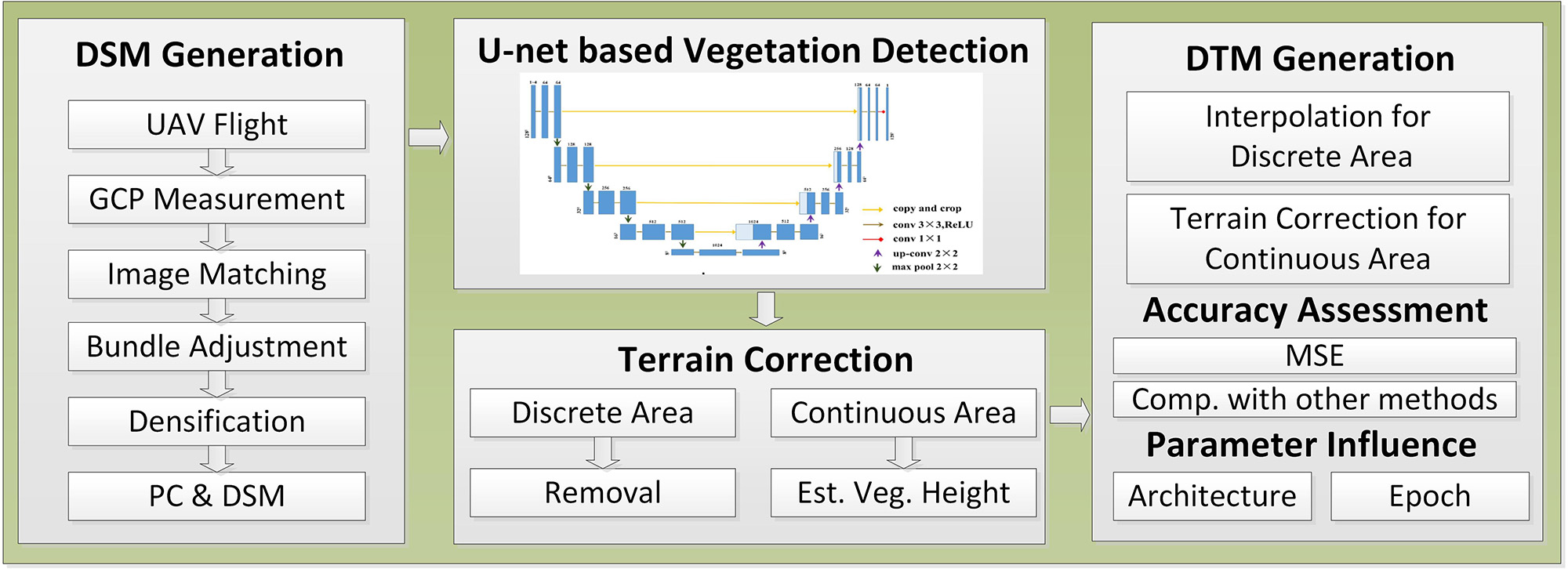
2. Materials and Methods
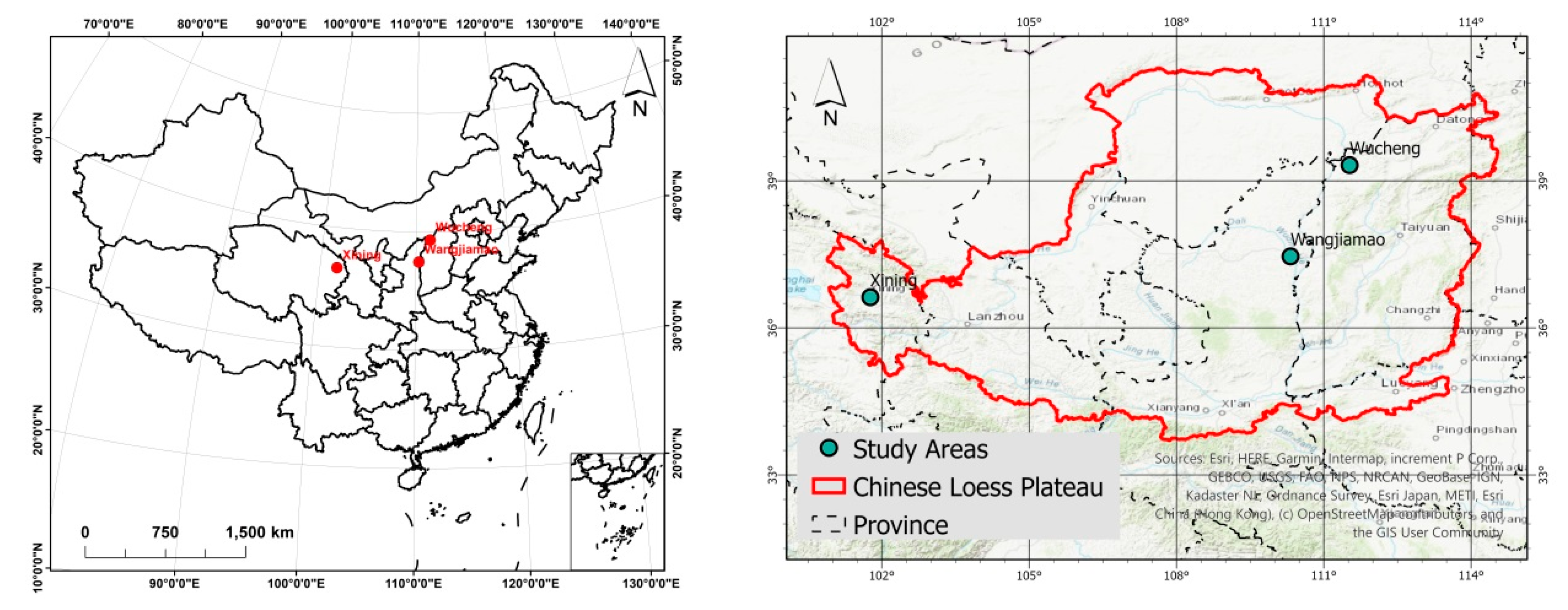
The proposed approach involved the following four steps—(1) UAV photogrammetry; (2) DL-based vegetation detection, (3) terrain correction, and (4) DTM generation. Accuracy assessment was conducted through the comparison between check points generated by global navigation satellite system (GNSS) unit and produced DTM elevation.

2.1. Study Site

Three study areas, namely, Xining (SA1), Wangjiamao (SA2), and Wucheng (SA3) located in Qinghai, Shaanxi, and Shanxi, respectively, were selected in the Loess Plateau of China (Figure 1) and represent loess hill and gully, loess hill and loess valley area, respectively. Among them, Wangjiamao and Wucheng cover the complete catchments, and Xining covers a hillslope area. All three study areas were covered with vegetation since the implementation of the ‘Grain for Green’ project (changing the agriculture to conservation area) from late 1990s [43,44]. Vegetation status of three different study areas varied in their types and spatial distributions. The vegetation in Xining was manmade for ecological protection from the formal cultivation, with an average interval distance of 2 m in the terraced slopes. While in the Wuchenggou and Wangjiawao areas, vegetation are more natural but some cash crops like apples and jujubes (Chinese dates), were still planted, with more dense horizontal distance around 1 m in the slopes. The basic geographic information is listed in Table 1.

2.2. Unmanned Aerial Vehicle (UAV) and Global Navigation Satellite System (GNSS) Field Data Collection

Image matching point clouds from UAV photogrammetry were used as the inputs for terrain modeling. Optical aerial photographs were captured using a DJI Inspire 1 microdrone [45] mounted with a digital camera system Zenmuse X5 [46] (15 mm focal length, RGB color, and 4096 × 2160 resolution), with a battery time of approximately 18 min, and could resist wind speeds of up to 10 m/s. Detailed flight information is shown in Table 2. Pix4D Capture flight planner software was used to plan a round-trip flight line along the study areas, and automatically collect images within certain designed flight distance. All flights were completed from 10 am to 2 pm, to ensure that the image quality would not be influenced by the shades. Ground control points (GCPs) in WGS-84 were obtained by the Topcon HiperSR RTK GNSS unit [47] (10 mm horizontal positioning accuracy and 15 mm vertical positioning accuracy), with a tripod, to ensure horizontal and vertical accuracy. Bundle adjustment was implemented in Pix4D Mapper software [48]. The point clouds were finally generated and interpolated into the grid digital surface model (DSM).
Eight targets along the vegetation in Xining (SA1) were designated as check points (CPs) for the uncertainty assessment of the final terrain modeling results. These targets were 1-m-wide boards painted in black and white in a diagonal chessboard pattern.

2.3. Deep Learning (DL)-Based Vegetation Detection

Most DL networks connect simple layers for data distillation. Input information passes through a layer of filter that increases the purity in distillation to achieve the desired result [49]. Convolutional neural network (CNN) is one of the representative algorithm structures of the deep neural network structure and is a feed-forward neural network usually used in object recognition, target detection, semantic segmentation, and other issues [50,51]. A typical structure for a CNN network, U-Net [52], was implemented for vegetation detection, because of its effectiveness and simplicity. U-net adopts the principle of gradient descent, propagates data information forward, and reverses propagation to correct the parameter weights and deviations [53]. Certain layers were changed and adjusted to specific terrain modeling tasks, on the basis of the existing U-Net structure.

2.3.1. Training Data Generation

DL is usually used in datasets with a large amount of data, and convolutional neural networks are suitable for processing relevant image data. Therefore, the U-Net model can generate a large number of images as input data. Here, input data were randomly cropped to ensure proper representation and eliminate the influence of manual selection. Random coordinate points were expanded, based on the desired image size. The crop range was calibrated, and the crop operation fully utilized the cell size and projected coordinate information.
Data enhancement is the process of generating new data for training, based on image nature, without actually collecting new samples. Convolution operations have translational invariance, and similar transformations such as rotation and scaling of vegetation data do not change the information characteristics of the vegetation data. Here, similar data outside the sample area chart were provided to the model to ensure data diversity. Random similar transformation, scale transformation, Gaussian blur, and image enhancement were performed for the crop data, in which the rotation allocation transformation matrix and 2D Gaussian function were treated as follows—Equations (1) and (2).
M = ( c o s θ s i n θ s i n θ c o s θ )
G ( x , y ) = 1 2 π σ 2 e ( x 2 + y 2 ) / 2 σ 2
where θ is the angle of rotation, and σ is the variance.
For the classification task, the training data was labeled as one-hot encoding logic category, namely, 1 for vegetation and 0 for non-vegetation. Manual work was first done for the labeling task at, based on the original point clouds. The RGB and additional elevation information of vegetation of the manmade labels of three study areas were then generated from the original image matching point cloud. All labels were divided into two groups for model training and validation. Forty percent of the dataset was randomly sampled as the training data. Since the DL requires a large amount of training samples, a tool was developed based on the ArcGIS Pro [54] software, using the python script for a multi-scale replicability of the training samples. Finally, 10,000 samples of 4 dimensions (R, G, B, Z) with 128 × 128 cells were automatically generated.

2.3.2. Feature Selection

The data for neural network represent a multidimensional feature array, also known as a tensor, a container for numerical data of images. All transformations learned by the neural network could be summed up as tensor operations for numerical data and formed matrix extension dimensions. Spectral information (R, G, and B values) and elevation provide theoretical feasibility for the division of vegetation. The training data generated by the original point clouds had an RGB value and underwent elevation, and the input data were normalized to reasonably eliminate the scale effect.

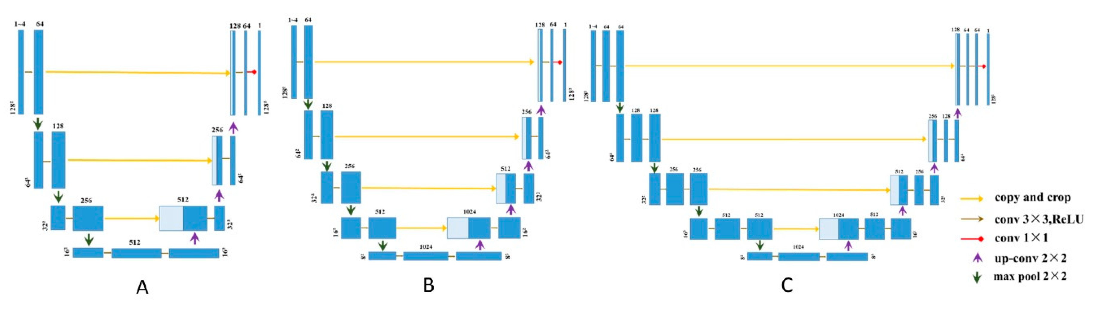
2.3.3. Design of the U-Net Network

An improved U-Net framework with a slightly altered structure was used for vegetation detection. The improved U-Net produced split maps of the same size as the input data and preserved the continuity of the resolution.
The predictive model describes the relationship between input x (features) and desired output (answer) y. The system ‘learns’ the relationship between data and output repeatedly through differential equations and random deviations and obtains the values of a series of unknown parameters, thus, forming a set of rules on its own. These rules are applied to a set of untrained data to allow the model to predict the corresponding set of answers. This process is the core architecture of the image segmentation task. With the use of the FCN (Fully Convolutional Networks, [55]) architecture, the simple representation of the relationship between the predictive output and the input is as follows—Equation (3).
ŷ = f ( j = 1 m ( w j ( i = 1 n w i x i θ n ) θ m ) )
where x is the input; ŷ is the forecast output; m is the number of hidden layers that determines the depth of the network to a certain extent and represents the complexity of the network; n is the number of neurons in each layer of network, and each neuron in the convolutional neural networks is represented as a filter (nine neurons in this study); w is expressed as a weight assigned to a neuron to connect input information for signaling; and f is an activation function for nonlinear mapping.
Three specific network structures architecture with different hyper-parameters were designed (Figure 2) for the vegetation detection tasks. In the down-sampling procedure, convolution was performed to extract features and activation values at different levels. Each convolution was based on the result of the previous layer of convolution, thus, bringing the model to a certain depth. Some convoluted feature values were de-dimensionalized from the input, through pooling, to reduce a large amount of computational consumption. The vegetation characteristics were summarized, and a wide range of features were extracted. The data were easily learned, and the model learning ability was enhanced. In the upper-sampling, the image size was expanded layer-by-layer to interpolate the feature maps at all levels. Details on the three model hyper-parameters are shown in Table 3.

2.3.4. Vegetation Detection Accuracy Assessment

The detection accuracy was assessed through a comparison with the reference. The reference data were manually interpolated from the original point cloud. The confusion matrix was applied to calculate the accuracy in the rasterized results.

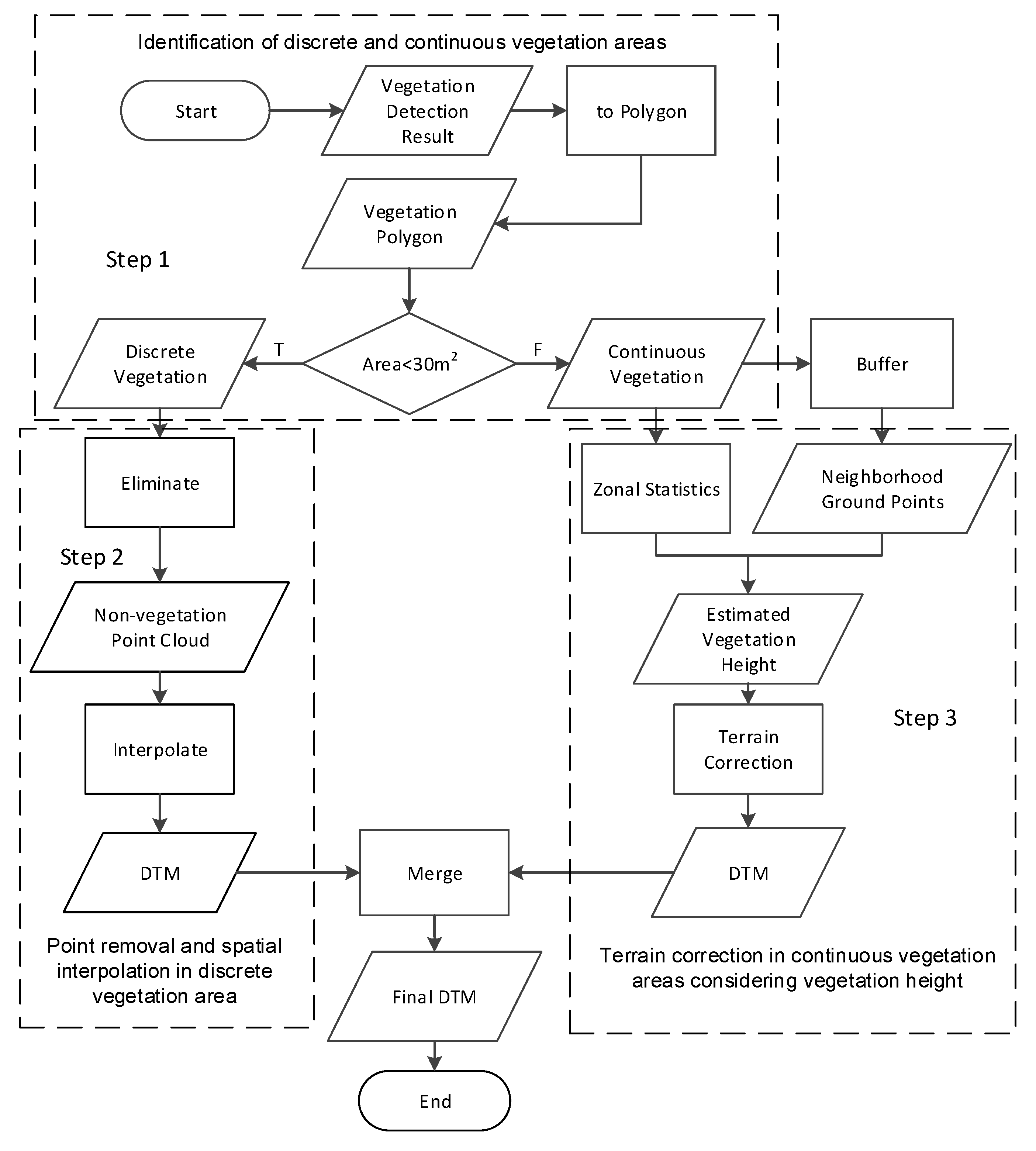
2.4. Terrain Correction

After vegetation detection, the terrain information could be modified using the vegetation results. In terrain modeling, the ability to reasonably eliminate the vegetation points, determined the accuracy of the DTM result. In urban areas, a cross-section is usually used to completely eliminate the vegetation point and then interpolate the complement point to obtain the DTM [56]. The ground is fitted in a 2D terrain plane, and the points higher than the plane are removed. However, this trend approach always fails, because the planes are difficult to estimate, due to the dramatic reliefs of the mountainous terrains (e.g., the Loess Plateau). The alternative practice for mountainous areas is usually to universally lower the vegetation points, based on the estimation of vegetation average height [37]. This method is effective for continuous vegetation in mountainous areas and maintaining the original terrain fluctuation, but is restricted for discrete vegetation in mountain areas, due to elevation fragmentation or convex terrain [57,58]. To solve this problem, this study divided the terrain correction into two scenarios, namely, discrete and continuous vegetation areas (Figure 3). The vegetation points in the discrete area were directly removed and then interpolated, and terrain correction was applied for the points in continuous areas.
Step 1: Identification of discrete and continuous vegetation areas.
The vegetation detection result was firstly rasterized then converted into polygon by the Raster to Polygon tool in ArcGIS Pro software [54]. A threshold of 30 m2 by expertise was then used to identify discrete and continuous vegetation areas. Vegetation areas of less than 30 m2 were classified as discrete, and those greater than 30 m2 were labeled as continuous.
Step 2: Point removal and spatial interpolation in discrete vegetation area.
The original point cloud obtained for the UAV photogrammetry represents a surface model including the vegetation information. To achieve a terrain model, all these vegetation points should be excluded. The points in the discrete vegetation area could be directly eliminated. Since the ‘holes’ after the removal were relatively small, it would not affect the overall trend of the terrain. Therefore, the terrain could then be interpolated.
Step 3: Terrain correction in continuous vegetation areas when considering vegetation height.
The commonly used local polynomial interpolation ignores its own terrain fluctuations. Thus, the elevation information would be lost when the points in the continuous vegetation area are simply removed. A possible solution was to estimate the terrain elevation and then modify the elevation of the vegetation points in the point cloud. With regard to the varying heights for each individual continuous vegetation area, an adaptive process with less human interaction was proposed. Vegetation height was estimated by the elevation in the 0.5 m buffer zone of each polygon. This could be achieved by the Zonal Statistics tool by ArcGIS Pro [54], using the original point clouds. The difference between the vegetation elevation point and the ground elevation in the polygonal area from DSMs was treated as the unified elevation value of the area, and the final fine DTM was obtained by subtracting the estimated mean height of each polygon.

2.5. Terrain Modeling Result Validation

Evaluating the elevated generated DTM is the key to measuring accurate terrain modeling results. To achieve the validation, a comparison between the final generated DTM with CPs from field survey by GNSS unit was conducted. The Xining area was selected for the validation.

3. Results

3.1. Vegetation Detection Results

Xining was selected for model training. After performance comparison for the designed U-Net network structures, the U-Net model C was finally chosen for vegetation detection. Details of three structures’ performance are discussed in following Section 4.1. After model training, the model was applied in two other study areas. Figure 4 shows the results for the three study areas.
Table 4 shows that the confusion matrix of vegetation detection results in three areas with the reference. The detection accuracies were acceptable at 90.9% for Xining, 96.4% for Wangjiamao, and 87.2% for Wucheng. The vegetation detection of Wucheng was not as highly accurate as for the other two areas because the tie points in the southwest corner of Wucheng were relatively insufficient during the automatic image matching. Hence, the accuracy of the original image matching point cloud was reduced.

3.2. Vegetation Identification Results

Identification was conducted in the three study areas, based on the adaptive treatment of discrete and continuous vegetation (Figure 5). The manmade vegetation spatial distribution patterns in Xining and the natural patterns in Wuchenggou and Wangjiawao were successfully identified. Vegetation height estimations ranged from 0.01 to 2.26 m (1.81 m in mean) in Xinning, 0.01 to 7.12 m in Wangjiamao (4.23 m in mean), and 0.66 to 6.38 m in Wucheng (4.21 m in mean), respectively.

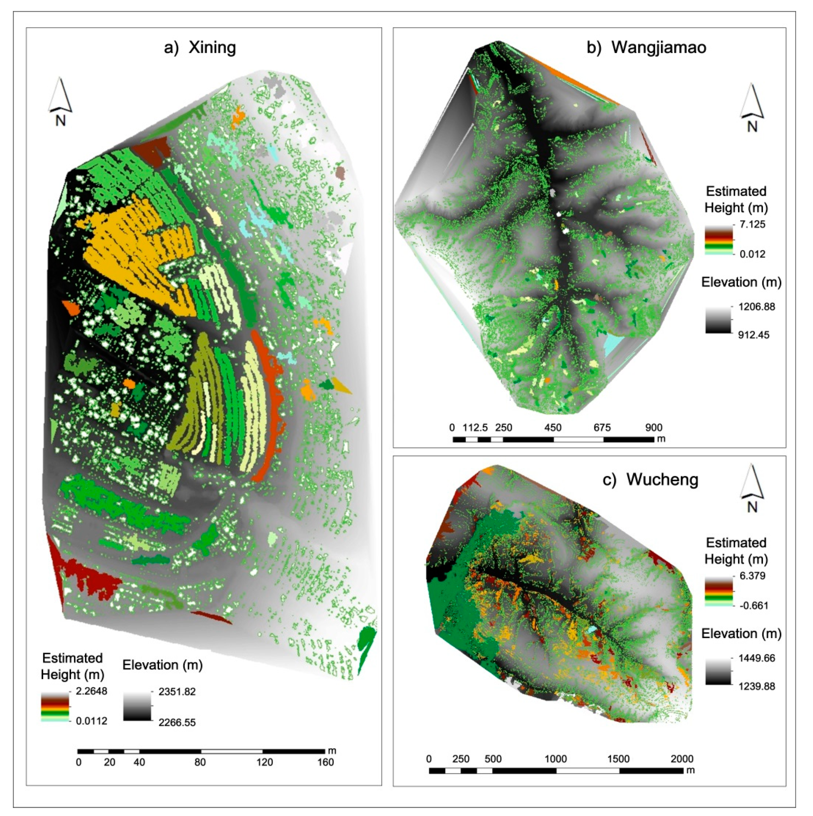
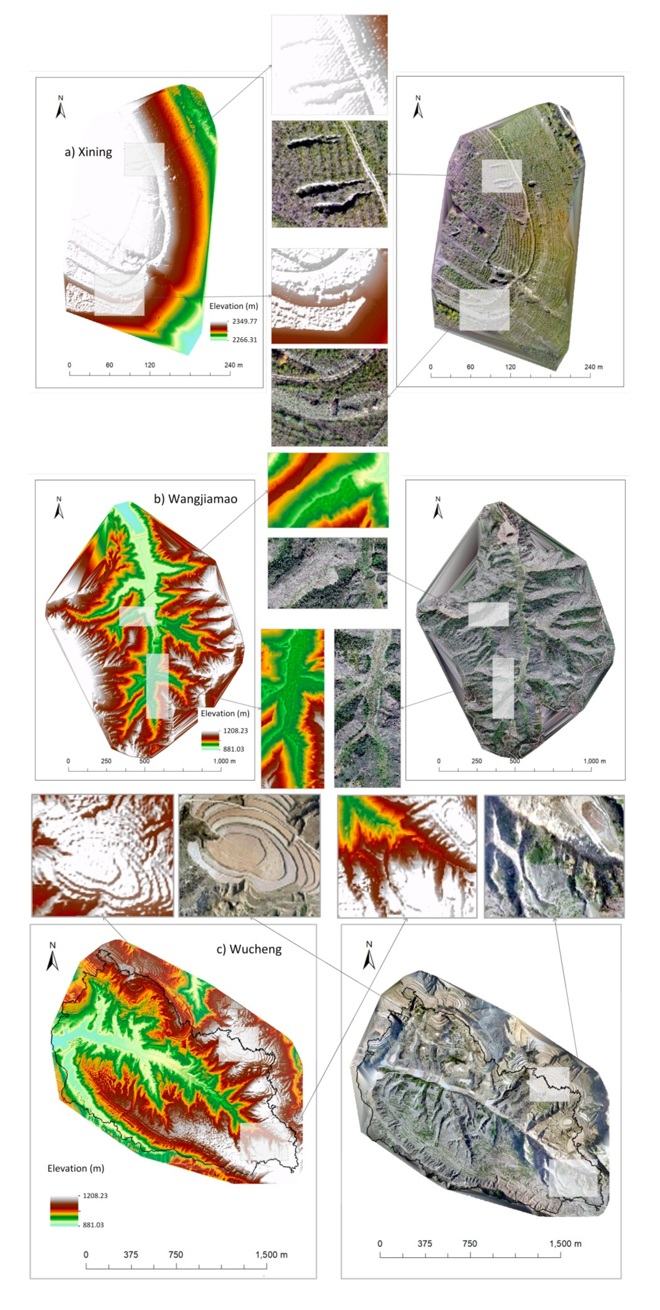
3.3. Terrain Correction Results

After the vegetation identification, terrain correction was done and DTMs with 1 m resolution were then interpolated (Figure 6). The proposed method removed the vegetation points without losing the terrain details and restored the fine DTM. Compared with orthophotos, the terrain reliefs were well presented in the modeling results. The smooth color rendering of DTMs indicated that the vegetation recognition removal was good, and DTM was visually refined.

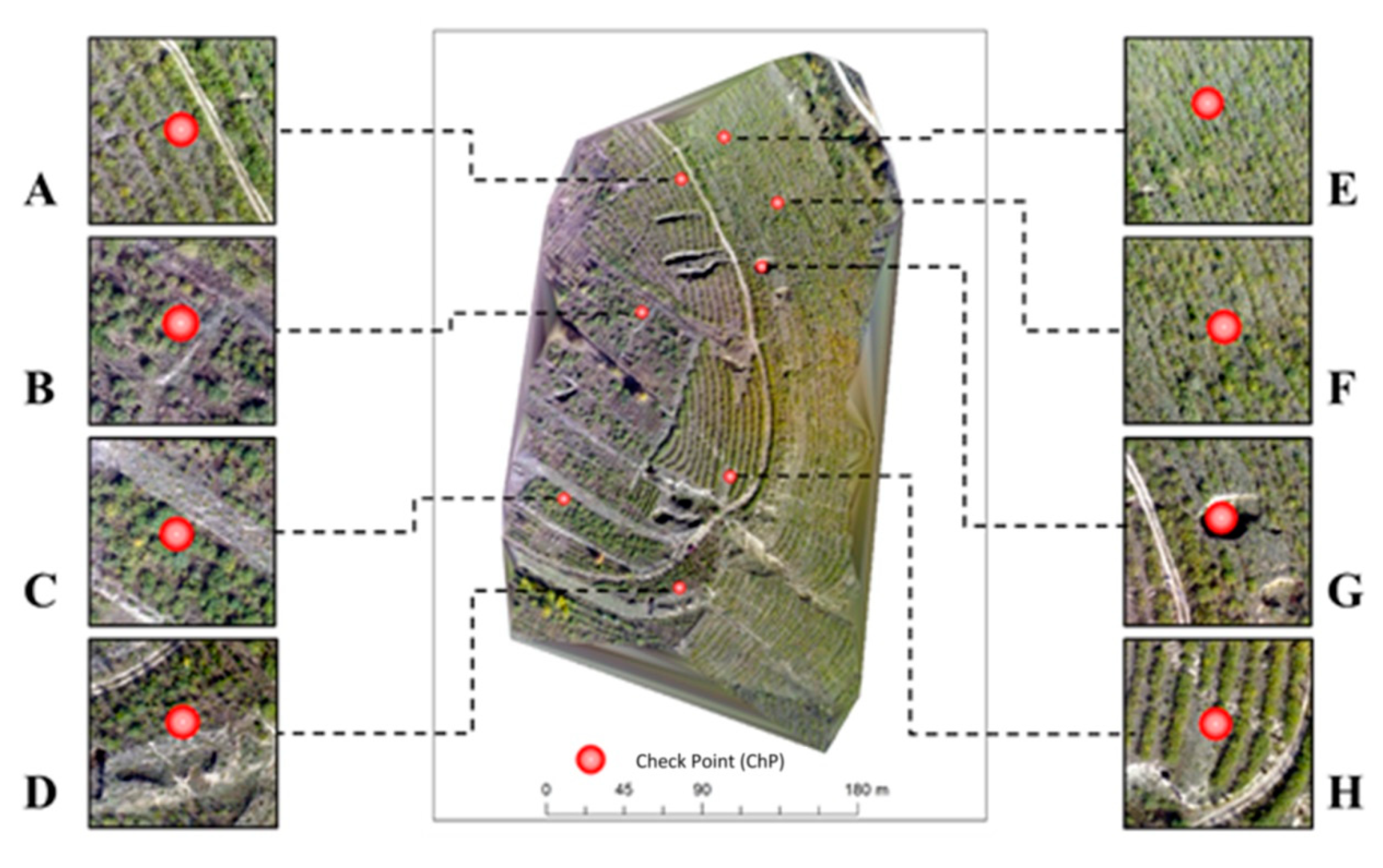
3.4. Terrain Modeling Result Validation with Field Measurement Data

Ground control points in Xining by field survey were elevated to verify the DTM results (Figure 7).
Table 5 shows the elevation comparison of the CPs. The MSE was 0.024 m, which met the standard of the accurate terrain modeling. Points D and H had the highest prediction accuracy, which were originally ground points. Correctly predicting the vegetation points ensured that the ground elevation values were preserved correctly. Point G failed the accurate elevation, because it was located at a hole even when the vegetation detection was not correct. The terrain correction of the remaining vegetation points was guaranteed.

4. Discussion

In this section, some extra analyses were conducted to discuss the key to the success of vegetation detection. Hyper-parameter (network structure and epoch) influence analysis was done at first to achieve an optimized parameter setting. The comparison with other two published methods (perceptron and adaptive filtering) was then done for a deeper analyses of the performance of our proposed vegetation detection method.

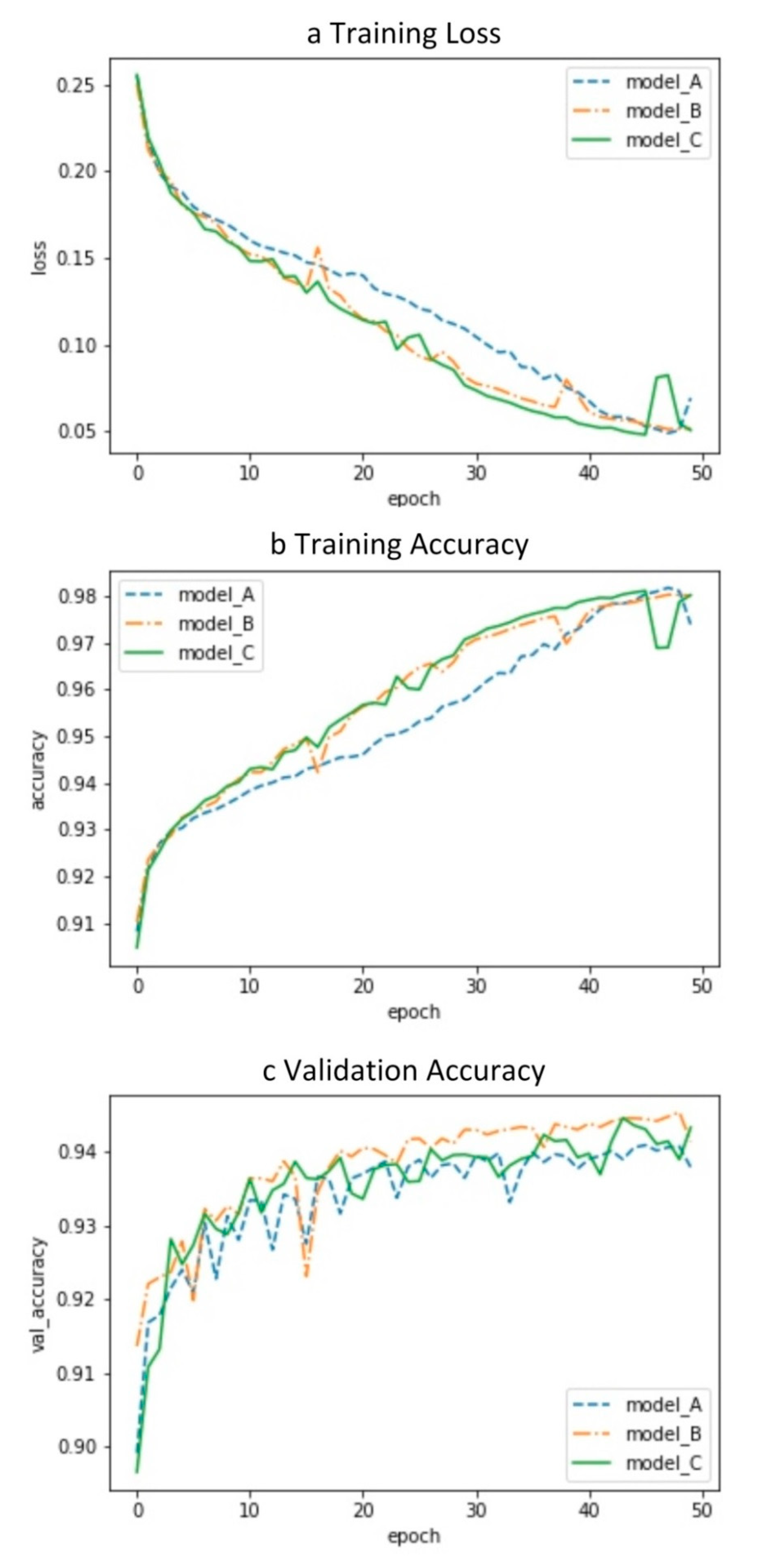
4.1. U-Net Hyper-Parameter Influence on Vegetation Detection Performance

The performance of the three designed different U-net networks was assessed in terms of training loss, validation accuracy, and training accuracy, to understand the influence of parameter and architecture on vegetation detection.
Figure 8a shows the training loss of the three models with different epoch settings. Model A is simple with a small network layer and capacity. Its training loss reached the local minimum at 48 epochs. The training loss of model B bounced at the 16th and 38th epochs, and was overall faster than that for Model A. The training loss of model C declined smoothly and reached the local minimum at the 45th epoch. Figure 8b shows the training accuracy of the three models with different epoch settings. All three models generally showed an increasing trend. Model A in the 8th epoch to 40th epoch did not meet the saturation. Model B in the 17th and 38th epochs showed a decline in training accuracy. Model C in the 45th epoch achieved the local maximum accuracy. Figure 8c shows the validation accuracy of the three models with different epoch settings. Model A had the lowest verification accuracy. Model B was moderately complex with convolution occurring during pooling, and its verification accuracy was high. However, a substantial decline in the 15th epoch to 0.92, indicated a slightly weakened stability of its performance. Model C was the most stable and accurate with a high accuracy of 0.94 at the 45th epoch (Figure 8c).
Model C with an epoch of 45 was selected for vegetation detection, due to its lowest loss function and highest accuracy during training and validation. When the network structure was large, the epoch should be increased appropriately to ensure that the parameters were updated. Merging combined the features of convolution and enhanced the upper sampling of data.

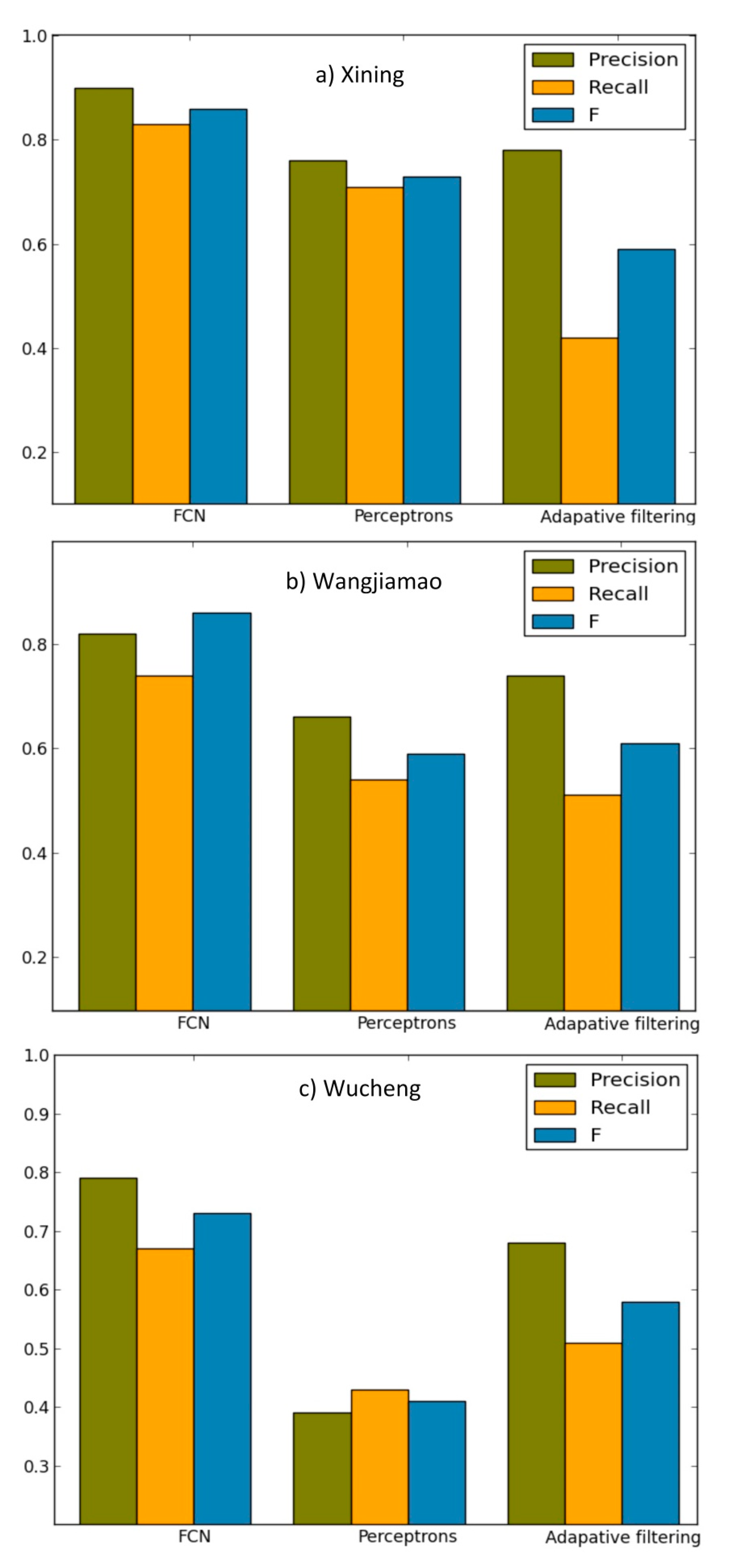
4.2. Comparison of Vegetation Detection Performance with Other Methods

Two other methods, namely, perceptron [59] and adaptive filtering [60] were selected for comparison to additional assessment of vegetation detection. Precision, recall, and F-score values were used for validation. Precision indicated the extent to which the extraction result represented the real target and the error of the model. Prediction was positive when the following values were obtained—true positive (TP) and false positive (FP)—which indicated the extraction of the correct vegetation grid. FP indicated that the ground sample was predicted as a vegetation sample, and FP was a ‘false positive’ situation. True negative (TN) was achieved when the results predicted for the ground was also a ground sample. Recall represents the extent to which real targets can be extracted and indicates the model’s leakage. Predicting vegetation as true (TP) and vegetation samples as ground samples were a false negative (FN), i.e., no vegetation samples were extracted. Precision was the number of samples that were positive relative to the predicted positive, and recall was relative to the number of positive samples in the original sample. The F-value was the reconciliation average of precision and recall. The formulas for precision, recall, and F-values were as follows (Equations (4)–(6).
Precision = TP/(TP + FP)
Recall = TP/(TP + FN)
F = 2 × Precision × Recall/(Precision + Recall)
Figure 9 shows the precision, recall, and F-value of the three methods. Our improved U-Net architecture had the highest values for all three study areas. Particularly, the best identification result was observed in Xining with a precision of 0.91. The performances of last two methods were seriously weaker than that of our improved U-Net architecture. Perceptron lacked the hidden layer and did not introduce random deviation. The final classification result was based on the hyperplane, which could not adapt to the complex terrain, resulting in a low accuracy for vegetation detection. Adaptive filtering was excessive in vegetation recognition, and its results depended on the sketched vegetation range. This phenomenon required the manual sketching of the training area, as a supervised area for vegetation recognition in each study area.

5. Conclusions

This study proposed a UAV photogrammetric framework for terrain modeling in dense vegetation areas. With the loess plateau of China as the study area, a DL and terrain correction ensemble method was proposed and applied. An improved U-net network for vegetation segmentation was presented. The feature combination of RGB+DSM was used for vegetation detection. According to four-fold cross-verification, the accuracy was 94.97%, and the model had a good generalization ability. The influence of U-Net architecture and parameter epoch setting on vegetation detection performance was also assessed. Comparison with other methods confirmed the better performance of the proposed technique. Fine DTM generation method for terrain modeling was also put forward. The vegetation area was divided into discrete and continuous, and adaptive terrain correction was proposed and realised. DTM accuracy was evaluated with the field measurements. This framework could be applied in dense vegetation, with an advantage of low-cost UAV photogrammetry when laser scanning was limited.

Author Contributions

Conceptualization, J.N. and K.X.; algorithm, J.N. and K.X.; classification analysis, J.N.; process the data, K.X.; writing—original draft preparation, J.N. and K.X.; writing—review and editing, H.D., J.S. and N.P.; supervision, L.X. and G.T.; funding acquisition, L.X. and G.T. All authors have read and agreed to the published version of the manuscript.

Funding

This work was financially supported by the Natural Science Foundation of China, grant numbers 41930102, 41971333, and the Priority Academic Program Development of Jiangsu Higher Education Institutions (No. 164320H116).

Acknowledgments

The authors sincerely thank for the comments from anonymous reviewers and members of the editorial team.

Conflicts of Interest

The authors declare no conflict of interest.

References

  1. Kulawardhana, R.W.; Popescu, S.C.; Feagin, R. Airborne lidar remote sensing applications in non-forested short stature environments: A review. Ann. For. Res. 2017, 60, 173–196. [Google Scholar] [CrossRef] [Green Version]
  2. Galin, E.; Guérin, É.; Peytavie, A.; Cordonnier, G.; Cani, M.; Benes, B.; Gain, J. A Review of Digital Terrain Modeling. Comput. Graph. Forum 2019, 38, 553–577. [Google Scholar] [CrossRef]
  3. Tmušić, G.; Manfreda, S.; Aasen, H.; James, M.R.; Gonçalves, G.; Ben Dor, E.; Brook, A.; Polinova, M.; Arranz, J.J.; Mészáros, J.; et al. Current Practices in UAS-based Environmental Monitoring. Remote Sens. 2020, 12, 1001. [Google Scholar] [CrossRef] [Green Version]
  4. Hladik, C.; Alber, M. Accuracy assessment and correction of a LIDAR-derived salt marsh digital elevation model. Remote. Sens. Environ. 2012, 121, 224–235. [Google Scholar] [CrossRef]
  5. Hladik, C.; Schalles, J.; Alber, M. Salt marsh elevation and habitat mapping using hyperspectral and LIDAR data. Remote Sens. Environ. 2013, 139, 318–330. [Google Scholar] [CrossRef]
  6. Tsouros, D.C.; Bibi, S.; Sarigiannidis, P.G. A review on UAV-based applications for precision agriculture. Information 2019, 10, 349. [Google Scholar] [CrossRef] [Green Version]
  7. Szabó, Z.; Tóth, C.A.; Holb, I.; Szabo, S. Aerial Laser Scanning Data as a Source of Terrain Modeling in a Fluvial Environment: Biasing Factors of Terrain Height Accuracy. Sensors 2020, 20, 2063. [Google Scholar] [CrossRef] [Green Version]
  8. Liu, K.; Ding, H.; Tang, G.; Na, J.; Huang, X.; Xue, Z.; Yang, X.; Li, F. Detection of Catchment-Scale Gully-Affected Areas Using Unmanned Aerial Vehicle (UAV) on the Chinese Loess Plateau. ISPRS Int. J. Geo-Inf. 2016, 5, 238. [Google Scholar] [CrossRef]
  9. Li, P.; Mu, X.; Holden, J.; Wu, Y.; Irvine, B.; Wang, F.; Gao, P.; Zhao, G.; Sun, W. Comparison of soil erosion models used to study the Chinese Loess Plateau. Earth-Science Rev. 2017, 170, 17–30. [Google Scholar] [CrossRef] [Green Version]
  10. Toutin, T.; Gray, L. State-of-the-art of elevation extraction from satellite SAR data. ISPRS J. Photogramm. Remote Sens. 2000, 55, 13–33. [Google Scholar] [CrossRef]
  11. Ludwig, R.; Schneider, P. Validation of digital elevation models from SRTM X-SAR for applications in hydrologic modeling. ISPRS J. Photogramm. Remote Sens. 2006, 60, 339–358. [Google Scholar] [CrossRef]
  12. Xu, F.; Jin, Y.-Q. Imaging Simulation of Polarimetric SAR for a Comprehensive Terrain Scene Using the Mapping and Projection Algorithm. IEEE Trans. Geosci. Remote Sens. 2006, 44, 3219–3234. [Google Scholar] [CrossRef]
  13. Sabry, R. Terrain and Surface Modeling Using Polarimetric SAR Data Features. IEEE Trans. Geosci. Remote Sens. 2016, 54, 1170–1184. [Google Scholar] [CrossRef]
  14. Spinhirne, J. Micro pulse lidar. IEEE Trans. Geosci. Remote Sens. 1993, 31, 48–55. [Google Scholar] [CrossRef]
  15. Petrie, G.; Toth, C.K. Introduction to Laser Ranging, Profiling, and Scanning. In Topographic Laser Ranging And Scanning: Principles And Processing, 2nd ed.; Shan, J., Toth, C.K., Eds.; CRC Press: Boca Raton, FL, USA, 2018; pp. 1–28. [Google Scholar]
  16. Milenković, M.; Ressl, C.; Piermattei, L.; Mandlburger, G.; Pfeifer, N. Roughness Spectra Derived from Multi-Scale LiDAR Point Clouds of a Gravel Surface: A Comparison and Sensitivity Analysis. ISPRS Int. J. Geo-Information 2018, 7, 69. [Google Scholar] [CrossRef] [Green Version]
  17. Benard, M. Automatic stereophotogrammetry: A method based on feature detection and dynamic programming. Photogrammetria 1984, 39, 169–181. [Google Scholar] [CrossRef]
  18. Van Zyl, J.J. The Shuttle Radar Topography Mission (SRTM): A breakthrough in remote sensing of topography. Acta Astronaut. 2001, 48, 559–565. [Google Scholar] [CrossRef]
  19. Rodríguez, E.; Morris, C.S.; Belz, J.E. A Global Assessment of the SRTM Performance. Photogramm. Eng. Remote Sens. 2006, 72, 249–260. [Google Scholar] [CrossRef] [Green Version]
  20. St-Onge, B.; Vega, C.; Fournier, R.A.; Hu, Y. Mapping canopy height using a combination of digital stereo-photogrammetry and lidar. Int. J. Remote Sens. 2008, 29, 3343–3364. [Google Scholar] [CrossRef]
  21. Latypov, D. Estimating relative lidar accuracy information from overlapping flight lines. ISPRS J. Photogramm. Remote. Sens. 2002, 56, 236–245. [Google Scholar] [CrossRef]
  22. Hodgson, M.E.; Bresnahan, P. Accuracy of Airborne Lidar-Derived Elevation. Photogramm. Eng. Remote Sens. 2004, 70, 331–339. [Google Scholar] [CrossRef] [Green Version]
  23. Salach, A.; Bakuła, K.; Pilarska, M.; Ostrowski, W.; Górski, K.; Kurczyński, Z. Accuracy Assessment of Point Clouds from LiDAR and Dense Image Matching Acquired Using the UAV Platform for DTM Creation. ISPRS Int. J. Geo-Inf. 2018, 7, 342. [Google Scholar] [CrossRef] [Green Version]
  24. Baltensweiler, A.; Walthert, L.; Ginzler, C.; Sutter, F.; Purves, R.S.; Hanewinkel, M. Terrestrial laser scanning improves digital elevation models and topsoil pH modelling in regions with complex topography and dense vegetation. Environ. Model. Softw. 2017, 95, 13–21. [Google Scholar] [CrossRef]
  25. Moon, D.; Chung, S.; Kwon, S.; Seo, J.; Shin, J. Comparison and utilization of point cloud generated from photogrammetry and laser scanning: 3D world model for smart heavy equipment planning. Autom. Constr. 2019, 98, 322–331. [Google Scholar] [CrossRef]
  26. Liu, P.; Chen, A.Y.; Huang, Y.-N.; Han, J.-Y.; Lai, J.-S.; Kang, S.-C.; Wu, T.-H.; Wen, M.-C.; Tsai, M.-H. A review of rotorcraft Unmanned Aerial Vehicle (UAV) developments and applications in civil engineering. Smart Struct. Syst. 2014, 13, 1065–1094. [Google Scholar] [CrossRef]
  27. Kanellakis, C.; Nikolakopoulos, G. Survey on Computer Vision for UAVs: Current Developments and Trends. J. Intell. Robot. Syst. 2017, 87, 141–168. [Google Scholar] [CrossRef] [Green Version]
  28. Zhong, Y.; Zhong, Y.; Xu, Y.; Wang, S.; Jia, T.; Hu, X.; Zhao, J.; Wei, L.; Zhang, L. Mini-UAV-Borne Hyperspectral Remote Sensing: From Observation and Processing to Applications. IEEE Geosci. Remote Sens. Mag. 2018, 6, 46–62. [Google Scholar] [CrossRef]
  29. Tsai, C.-H.; Lin, Y.-C. An accelerated image matching technique for UAV orthoimage registration. ISPRS J. Photogramm. Remote Sens. 2017, 128, 130–145. [Google Scholar] [CrossRef]
  30. Ziquan, W.; Yifeng, H.; Mengya, L.; Kun, Y.; Yang, Y.; Yi, L.; Sim-Heng, O. A small uav based multi-temporal image registration for dynamic agricultural terrace monitoring. Remote Sens. 2017, 9, 904. [Google Scholar]
  31. Wan, X.; Liu, J.; Yan, H.; Morgan, G.L. Illumination-invariant image matching for autonomous UAV localisation based on optical sensing. ISPRS J. Photogramm. Remote Sens. 2016, 119, 198–213. [Google Scholar] [CrossRef]
  32. Jiang, S.; Jiang, W. Hierarchical motion consistency constraint for efficient geometrical verification in UAV stereo image matching. ISPRS J. Photogramm. Remote Sens. 2018, 142, 222–242. [Google Scholar] [CrossRef]
  33. Zhao, J.; Zhang, X.; Gao, C.; Qiu, X.; Tian, Y.; Zhu, Y.; Cao, W. Rapid Mosaicking of Unmanned Aerial Vehicle (UAV) Images for Crop Growth Monitoring Using the SIFT Algorithm. Remote Sens. 2019, 11, 1226. [Google Scholar] [CrossRef] [Green Version]
  34. Colomina, I.; Molina, P. Unmanned aerial systems for photogrammetry and remote sensing: A review. ISPRS J. Photogramm. Remote Sens. 2014, 92, 79–97. [Google Scholar] [CrossRef] [Green Version]
  35. Yu, H.; Li, G.; Zhang, W.; Huang, Q.; Du, D.; Tian, Q.; Sebe, N. The Unmanned Aerial Vehicle Benchmark: Object Detection, Tracking and Baseline. Int. J. Comput. Vis. 2019, 128, 1141–1159. [Google Scholar] [CrossRef]
  36. Guisado-Pintado, E.; Jackson, D.W.; Rogers, D. 3D mapping efficacy of a drone and terrestrial laser scanner over a temperate beach-dune zone. Geomorphology 2019, 328, 157–172. [Google Scholar] [CrossRef]
  37. Meng, X.; Shang, N.; Zhang, X.; Li, C.; Zhao, K.; Qiu, X.; Weeks, E. Photogrammetric UAV Mapping of Terrain under Dense Coastal Vegetation: An Object-Oriented Classification Ensemble Algorithm for Classification and Terrain Correction. Remote Sens. 2017, 9, 1187. [Google Scholar] [CrossRef] [Green Version]
  38. Kolarik, N.E.; Gaughan, A.E.; Stevens, F.R.; Pricope, N.G.; Woodward, K.; Cassidy, L.; Salerno, J.; Hartter, J. A multi-plot assessment of vegetation structure using a micro-unmanned aerial system (UAS) in a semi-arid savanna environment. ISPRS J. Photogramm. Remote Sens. 2020, 164, 84–96. [Google Scholar] [CrossRef] [Green Version]
  39. Jensen, J.L.R.; Mathews, A.J. Assessment of Image-Based Point Cloud Products to Generate a Bare Earth Surface and Estimate Canopy Heights in a Woodland Ecosystem. Remote Sens. 2016, 8, 50. [Google Scholar] [CrossRef] [Green Version]
  40. Gruszczyński, W.; Matwij, W.; Ćwiąkała, P. Comparison of low-altitude UAV photogrammetry with terrestrial laser scanning as data-source methods for terrain covered in low vegetation. ISPRS J. Photogramm. Remote Sens. 2017, 126, 168–179. [Google Scholar] [CrossRef]
  41. Ressl, C.; Brockmann, H.; Mandlburger, G.; Pfeifer, N.; Camillo, R.; Herbert, B.; Gottfried, M.; Norbert, P. Dense Image Matching vs. Airborne Laser Scanning—Comparison of two methods for deriving terrain models. Photogramm. Fernerkund. Geoinf. 2016, 2016, 57–73. [Google Scholar] [CrossRef]
  42. Manfreda, S.; McCabe, M.F.; Miller, P.E.; Lucas, R.; Pajuelo Madrigal, V.; Mallinis, G.; Ben-Dor, E.; Helman, D.; Estes, L.; Ciraolo, G.; et al. On the Use of Unmanned Aerial Systems for Environmental Monitoring. Remote Sens. 2018, 10, 641. [Google Scholar] [CrossRef] [Green Version]
  43. Feng, Z.; Yang, Y.; Zhang, Y.; Zhang, P.; Li, Y. Grain-for-green policy and its impacts on grain supply in West China. Land Use Policy 2005, 22, 301–312. [Google Scholar] [CrossRef]
  44. Delang, C.O.; Yuan, Z. China’s Reforestation and Rural Development Programs. In China’s Grain for Green Program; Springer International Publishing: Cham, Switzerland, 2016; pp. 22–23. [Google Scholar]
  45. DJI Inspire 1. Available online: https://www.dji.com/inspire-1?site=brandsite&from=landing_page (accessed on 28 September 2020).
  46. Zenmuse X5. Available online: https://www.dji.com/zenmuse-x5?site=brandsite&from=landing_page (accessed on 28 September 2020).
  47. HiPer SR. Available online: https://www.topcon.co.jp/en/positioning/products/pdf/HiPerSR_E.pdf (accessed on 28 September 2020).
  48. Pix4D. Available online: https://www.pix4d.com/product/pix4dmapper-photogrammetry-software (accessed on 28 September 2020).
  49. Chollet, F. What is deep learning? In Deep Learning with Python; Manning Publications: Shelter Island, NY, USA, 2017; pp. 8–9. [Google Scholar]
  50. Zhang, W.; Itoh, K.; Tanida, J.; Ichioka, Y. Parallel distributed processing model with local space-invariant interconnections and its optical architecture. Appl. Opt. 1990, 29, 4790–4797. [Google Scholar] [CrossRef]
  51. Valueva, M.; Nagornov, N.; Lyakhov, P.; Valuev, G.; Chervyakov, N. Application of the residue number system to reduce hardware costs of the convolutional neural network implementation. Math. Comput. Simul. 2020, 177, 232–243. [Google Scholar] [CrossRef]
  52. Ronneberger, O.; Fischer, P.; Brox, T. U-net: Convolutional networks for biomedical image segmentation. In Proceedings of the 18th International Conference on Medical Image Computing and Computer-Assisted Intervention; Springer: New York, NY, USA, 2015; pp. 234–241. [Google Scholar]
  53. Erdem, F.; Avdan, U. Comparison of Different U-Net Models for Building Extraction from High-Resolution Aerial Imagery. Int. J. Environ. Geoinf. 2020, 7, 221–227. [Google Scholar] [CrossRef]
  54. Arcgis Pro. Available online: https://www.esri.com/en-us/arcgis/products/arcgis-pro/overview (accessed on 28 September 2020).
  55. Long, J.; Shelhamer, E.; Darrell, T. Fully convolutional networks for semantic segmentation. In Proceedings of the IEEE Conference on Computer Vision and Pattern Recognition, Boston, MA, USA, 8–10 June 2015; pp. 3431–3440. [Google Scholar]
  56. Wang, R.; Peethambaran, J.; Chen, D. LiDAR Point Clouds to 3-D Urban Models: A Review. IEEE J. Sel. Top. Appl. Earth Obs. Remote Sens. 2018, 11, 606–627. [Google Scholar] [CrossRef]
  57. Zlinszky, A.; Boergens, E.; Glira, P.; Pfeifer, N. Airborne Laser Scanning for calibration and validation of inshore satellite altimetry: A proof of concept. Remote Sens. Environ. 2017, 197, 35–42. [Google Scholar] [CrossRef] [Green Version]
  58. Klápště, P.; Fogl, M.; Barták, V.; Gdulov, K.; Urban, R.; Moudrý, V. Sensitivity analysis of parameters and contrasting performance of ground filtering algorithms with UAV photogrammetry-based and LiDAR point clouds. Int. J. Digit. Earth 2020, 1–23. [Google Scholar] [CrossRef]
  59. Kwak, Y.-T. Segmentation of objects with multi layer perceptron by using informations of window. J. Korean Data Inf. Sci. Soc. 2007, 18, 1033–1043. [Google Scholar]
  60. Han, H.; Yulin, D.; Qing, Z.; Jie, J.; Xuehu, W.; Li, Z.; Wei, T.; Jun, Y.; Ruofei, Z. Precision global dem generation based on adaptive surface filter and poisson terrain editing. Acta Geod. Cartogr. Sin. 2019, 48, 374. [Google Scholar]
Figure 1. Study areas.
Remotesensing 12 03318 g001
Figure 2. Three designed U-net model structures.
Remotesensing 12 03318 g002
Figure 3. Workflow of terrain correction.
Remotesensing 12 03318 g003
Figure 4. Vegetation detection result. (a) Xining; (b) Wangjiamao; and (c) Wucheng.
Remotesensing 12 03318 g004
Figure 5. Vegetation identification results. (a) Xining; (b) Wangjiamao; (c) Wucheng. Base map is the digital surface model (DSM), and the estimated vegetation height is colored.
Remotesensing 12 03318 g005
Figure 6. Digital terrain model (DTM) (left) and orthophoto (right) results after terrain corrections. (a) Xining; (b) Wangjiamao; (c) Wucheng. Two detailed windows of each study areas are enlarged.
Remotesensing 12 03318 g006
Figure 7. Elevation uncertainty assessment in Xining.
Remotesensing 12 03318 g007
Figure 8. DTM results after terrain corrections. (a) training loss, (b) training accuracy, and (c) validation accuracy of the three different network structures, with different epoch settings.
Remotesensing 12 03318 g008
Figure 9. Comparison of accuracy under three methods (FCN by our U-net based method, Perceptrons by Kwak et al., 2007 and Adapative filtering by Hu et al., 2019). (a) Xining; (b) Wangjiamao; and (c) Wucheng. Dark green, orange, and blue bars are Precision, Recall, and F-value respectively.
Remotesensing 12 03318 g009
Table 1. Geography of study areas.
Xining (SA1)Wangjiamao (SA2)Wucheng (SA3)
Location36°39′N101°43′E37°34′20″N~37°35′10″N
110°21′50″E~110°22′40″E
39°15′51″N~39°16′57″N
111°33′21″E~111°34′48″E
Area0.07 km22.21 km23.17 km2
Elevation2266–2348 m1011–1195 m1238–1448 m
LandformLoess hill and gullyLoess hillLoess valley
ClimateSemi-arid (BSh)Semi-arid (BSh)Semi-arid (BSh)
Annual Temperature6.5℃9.7℃8℃
Precipitation327 mm/y486 mm/y~450 mm/y
VegetationWeedShrubArbor
Main vegetation typeRhamnus erythroxylon, ArtemisiaHaloxylon ammodendron, Ziziphus jujubaHippophae, Malus domestica
Vegetation height0.5–2 m0.5–6 m0.5–6 m
Table 2. Unmanned aerial vehicle (UAV) flight information of three study areas.
XiningWangjiamaoWucheng
Flight date2017.10.242019.08.202018.04.26
Flight height50 m150 m200 m
Photo gained in total80420680
Flight overlapping80%80%80%
Side overlapping70%70%70%
Ground sampling distance2.31 cm4.36 cm8.06 cm
Ground Control Points in total71819
Mean RMS of GCPs0.011 m0.014 m0.018 m
Point amount from dense matching83234179176179956200
Table 3. Comparison of model hyper-parameters.
NetworkABC
Layers5610
Down-sampling3× 3 × 64 (×128, ×256, ×512, ×512)3 × 3 × 64 (×128, ×256, × 512, ×1024, ×1024)Double B
Up-sampling3 × 3 × 256 (×128,×64)3×3×512(×256, ×128, ×64)Double B
Pooling(2 × 2) × 3(2 × 2)× 4(2 × 2) × 4
Jump connection3 times4 times4 times
Table 4. Confusion matrix of vegetation detection results in three areas for architecture C.
Detection (In Cells)
XiningWangjiamaoWuchenggou
GroundVegetationGroundVegetationGroundVegetation
ReferenceGround4,457,886 (62.3%)225,949 (3.1%)127,645,071 (90.0%)2,049,627 (1.4%)2,095,418 (69.4%)135,462 (4.5%)
Vegetation425,710 (6.0%)2,039,464 (28.6%)3,181,941 (2.2%)9,075,223 (6.4%)252,464 (8.3%)535,952 (17.8%)
Table 5. Elevation comparison of CPs.
SampleReference/mResult/mError/m
A2343.2462343.5180.272
B2343.2832343.4240.141
C2339.2752338.772−0.497
D2335.7182335.7390.021
E2328.0192327.967−0.948
F2317.5862317.6990.113
G2331.0992332.1971.098
H2340.8062340.800−0.006

