Abstract
Structure-from-motion (SfM) photogrammetry enables the cost-effective digital characterisation of seismic- to sub-decimetre-scale geoscientific samples. The technique is commonly used for the characterisation of outcrops, fracture mapping, and increasingly so for the quantification of deformation during geotechnical stress tests. We here apply SfM photogrammetry using off-the-shelf components and software, to generate 25 digital drill core models of drill cores. The selected samples originate from the Longyearbyen CO2 Lab project’s borehole DH4, covering the lowermost cap rock and uppermost reservoir sequences proposed for CO2 sequestration onshore Svalbard. We have come up with a procedure that enables the determination of bulk volumes and densities with precisions and accuracies similar to those of such conventional methods as the immersion in fluid method. We use 3D printed replicas to qualitatively assure the volumes, and show that, with a mean deviation (based on eight samples) of 0.059% compared to proven geotechnical methods, the photogrammetric output is found to be equivalent. We furthermore splice together broken and fragmented core pieces to reconstruct larger core intervals. We unwrap these to generate and characterise 2D orthographic projections of the core edge using analytical workflows developed for the structure-sedimentological characterisation of virtual outcrop models. Drill core orthoprojections can be treated as directly correlatable to optical borehole-wall imagery data, enabling a direct and cost-effective elucidation of in situ drill core orientation and depth, as long as any form of borehole imagery is available. Digital drill core models are thus complementary to existing physical and photographic sample archives, and we foresee that the presented workflow can be adopted for the digitisation and digital storage of other types of geological samples, including degradable and dangerous ice and sediment cores and samples.
1. Introduction
Structure-from-motion (SfM) photogrammetry has led to the rapid evolution of cost-effective digital characterisation of geological, palaeontological and archaeological sites [1,2]. This method has significant potential for the geoscientific community. Through SfM, digital characterisation is readily extended to include sub-decimetre-scale geoscientific samples, and allows for the quantification of data and the subsequent integration of big-data workflows. Though limited to command-line interfaces as recently as a decade ago, technological advances, coupled with improvements in software graphical user interfaces, now enable high precision and accurate 3D shape reconstruction through use of off-the-shelf photogrammetry software (e.g., Pix4D, Metashape, Trimble InPho, WebODM). Digital reconstructions can be used to visualise reservoir analogues (e.g., [3]), are accurate enough for large-scale bulk volumetric calculations (e.g., [4]), and can be used for the characterisation, digital storage, and the reproduction (i.e., 3D printing) of samples (e.g., [5]). Industrial applications of SfM are widespread in the mining industry (e.g., [6]), agriculture and forestry (e.g., [7]), snow science (e.g., [8]), geotechnical monitoring (e.g., [9]), and even in healthcare (e.g., [10]).
Digitisation not only allows for the digital characterisation of rock samples and outcrops, but also for the repeatability of experiments. The latter is often a limitation of destructive analytical methods [5]. Non-destructive characterisation methods are especially important for the geological analysis of drill cores acquired during industrial and scientific drilling. Drill cores are difficult and expensive to obtain, and provide a unique (1D) window into subsurface conditions, providing direct evidence of a multitude of geological and petrophysical properties. Many of these are obtained through destructive testing, though some of which are increasingly assessed through digital imaging and processing, including magnetic resonance imaging (e.g., [11]) and CT scanning (e.g., [12]).
The application of full-sample photogrammetry produces a comprehensive visual record of (surface) conditions. Identifiable features hereof can be measured and assessed digitally, and integrated with 3D modelling and reverse engineering processes (e.g., [13]) long after the loss of the original. SfM photogrammetry has been fully implemented to anything from outcrop to coin-scales in archaeology and palaeontology (e.g., [14,15,16]). The adaptation of photogrammetry in the geosciences to study the sub-metre scale has generally been slow, although the technique is widely used in outcrop-scale digitisations during stratigraphic, structural, and sedimentological characterisations (e.g., [17,18,19,20]). In geotechnics, SfM is increasingly being used to determine in situ stresses during deformation tests through changes in local volumes and fracture mapping [21,22,23,24,25]. Although the potential of digital rock models has been outlined (e.g., [26]), current geoscientific workflows fall short of the full and complete digitisation of samples as, for example, applied in palaeontology (e.g., [27]). Digitisations with sub-millimetre resolutions have for a long time only been achievable through complex workflows and expensive setups [28], but can increasingly be afforded through consumer-grade software and hardware solutions.
Through this contribution we aim to introduce an efficient and high resolution SfM photogrammetry workflow as a tool for the full digitisation of centimetre-scale geological samples, by focusing on the generation of digital (drill) core models (DCMs). Core material can be very fragile, with especially shale-rich intervals affected by operational and storage-related wear and tear. Secondly, we outline the potential of the workflow by discussing technical and scientific applications that include cost- and time-effective bulk volume and density assessments, and drill core characterisation and reconstruction. Finally, we use unwrapped, 2D orthographic core reprojections and integrate them with borehole televiewer data to re-align and elucidate the in situ drill core positions and orientations. To enhance accessibility and uptake, we use off-the-shelf and inexpensive, consumer-grade components to contribute to the investigative operations of the pilot-scale, onshore carbon, capture and storage (CCS) study ([29], and references therein) in Longyearbyen, Svalbard, Arctic Norway (Figure 1).
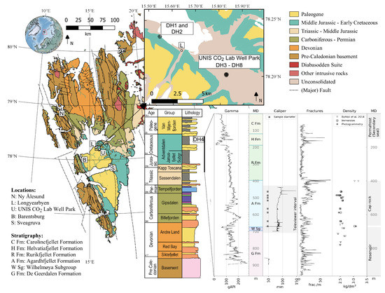
Figure 1.
Location and geological map of Svalbard and its main settlements. The inset shows a close-up of Longyearbyen, with the UNIS CO2 Lab Well Park. The interval covered by DH4 is indicated on the stratigraphic column, and a selection of available wireline logging, the televiewer interval, and available core-density data are shown. The fracture track is an image-based interpretation from Braathen et al. [30], and includes drilling-induced fractures. The stratigraphic column is based on an unpublished figure by Arild Andresen (UiO). Geological map data provided by the Norwegian Polar Institute.
2. Materials and Methods
Using drill cores from the Longyearbyen CO2 Lab ([29], and references therein), we implement experimental DCMs and procedures to (1) more cost- and time-effectively acquire accurate drill core bulk densities, (2) provide undistorted, 2D orthographic drill core projections (i.e., unwrapped 3D DCMs, directly correlatable to televiewer data), (3) digitally map tectonic and sedimentary features, (4) determine physical core (re-)orientation through integration with acoustic televiewer data, and, (5) lay the foundation for an accessible digital drill core laboratory. Figure 2 provides a schematic overview of these steps in a simple look-up flowchart.
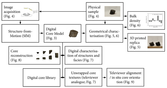
Figure 2.
Flowchart of the developed workflow to generate digital (drill) core models (DCMs) and associated products.
2.1. The Longyearbyen CO2 Lab Data Sets and Sample Collection
The Longyearbyen CO2 Lab was established by the University Centre in Svalbard (UNIS) along with industrial partners in 2007. The primary focus was to appraise the potential reservoir and cap rock units to store CO2 produced by Longyearbyen’s coal-fuelled power plant ([29,30], and references therein). Eight boreholes were drilled and fully cored, providing approximately 4.5 km of physical drill core samples of varying diameter (ranging from 78 to 28 mm due to telescopic borehole casing) [29,30]. Numerous multi-physical data sets (e.g., temperature, sonic, gamma ray), rock properties (e.g., permeability, porosity) and rock samples have been acquired and tested (e.g., [29,30,31,32,33,34]).
The slimhole operations did not, however, allow full wireline characterisation and, for instance, only qualitative density measurements were taken [35]. Existing bulk density data derived through geotechnical characterisation (e.g., [34]) provide insufficient coverage to calibrate the entire log suite, as required for instance for seismic modelling [36]. The acquisition of additional bulk density data is therefore needed to quantify a continuous density log, which is vital to the on-going characterisation of the cap rock sequences.
Drill core samples were selected from the interval for which wireline logging (including acoustic televiewer) is available, and are listed in Table 1. This interval covers the lowermost cap rock and uppermost reservoir sequences (approximately 440 to 700 m MD; DH4), represented by the shale-dominated, Late-Jurassic Agardhfjellet Formation [37] and the underlying Norian-Bathonian Wilhelmøya Subgroup [38,39], respectively [29,30]. The samples range from 4.7 cm (Agardhfjellet Fm) to 4.1 cm (Wilhelmøya Subgroup) in diameter (Figure 1). Physical sample shapes include right-cylinders and half-cores, as well as a range of drill core fragments of various sizes (Figure 3). With the exception of DH4-643 and DH4-673, which consist primarily of silt and sandstone, the lithologies are dominated by the cap rock shale. Finally, DH4-503, DH4-591, and DH4-673 feature slip surfaces and/or natural fractures, and the highly fractured DH4-487.5* (including sub-fragments) was selected for reconstruction based on the recognition of the corresponding anomaly observed in acoustic televiewer data. Figure 1 provides a schematic compilation of both existing data sets, as well as intervals targeted by this study.

Table 1.
Overview of sample origins, dimensions, and SfM parameters, results and errors. Refer to the main text for processing settings. AM: Agisoft Metashape marker; ArUco: ArUco marker.
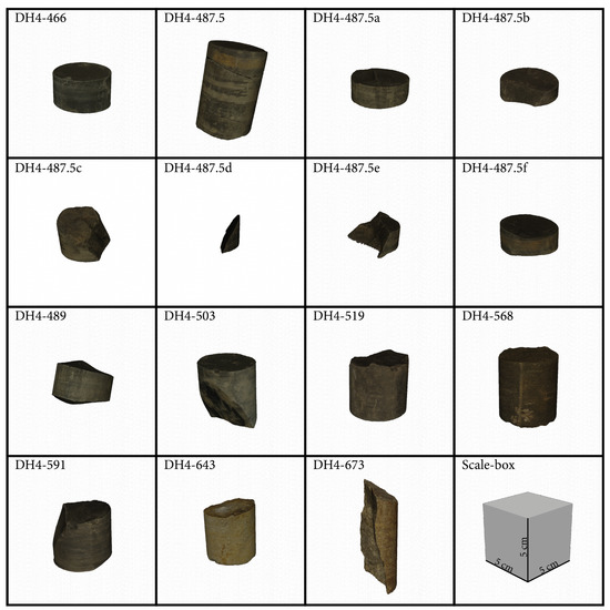
Figure 3.
An overview of the digitised DCMs (excluding sub-fragments and DH4-591w), universally scaled. Dimensions and origins are available in Table 1.
2.2. Digital Image Acquisition
Digital images were acquired using a computer-controlled system camera (Sony ILCE6300/S) coupled with either a 18-135 mm (Sony SEL18135) or 35 mm (Sony SEL35F18.AE) lens in conjunction with a well-lit turntable on uniform white background. The acquisition was carried out by placing the camera in front of a turntable loaded with a sample and evenly illuminated along the camera-sample axis (Figure 4A). The camera-sample distance was kept at approximately 40 cm, and aperture (highest), shutter speed, and focal length were kept constant for each sample. Both camera and lighting elements were warmed-up prior to image acquisition to ensure stabilised conditions had been reached prior to sampling.
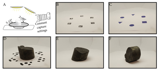
Figure 4.
Overview of the digital image acquisition step. Using a well-lit turn table (A), the sample was captured from 5–15-degree angle intervals for each of the three orientations (top-down, (D); down-top, (E); and, sideways, (F)). Markers (B,D) and (coordinate-less) calibration aids (C) were used for top-down and down-top positions.
Image acquisition commenced by photographing the sample in top-down (Figure 4D), sideways (Figure 4F), and down-top (Figure 4E) positions at 5 to 15 degree intervals of the turntable circumference, resulting in approximately 25 to 35 images per position. A ground control point (GCP)-sheet was added during photography of the top-down position, featuring up to six GCPs with pre-established distances. The marker sheets featured either 12 bit Metashape (Figure 4D; [40]) or ArUco-based (Figure 4B; [41]) markers. While left blank for larger samples, the GCPs were substituted with 6 distinctive icons (i.e., calibration aids; Figure 4C) during photography of the down-top position for smaller samples to enhance accuracy during the SfM processing step.
2.3. SfM Processing
Prior to the workflow optimisation implemented for DH4-487.5* and DH4-591w samples, a semi-automated marker detection and masking sequence was used that featured proprietary Metashape 12-bit markers. This procedure relied on Metashape’s built-in marker detection tools, and marker positions and photos were manually finetuned and masked. For DH4-487.5* samples and more recent digitisations, OpenCV Python libraries [42] and the Metashape Python API [43] were used to automate the procedure to:
- (1)
- automatically detect (ArUco) GCPs and assign their x,y-pixel coordinates;
- (2)
- create frame-encompassing masks isolating the GCPs, calibration aids, and the sample, effectively filtering out the white background; and,
- (3)
- apply real-world distances between markers derived from a marker-layout file.
Subsequently, the images were quality-inspected and used for the reconstruction of a 3D textured mesh using the Metashape photogrammetry software suite [40]. The reconstruction process was conducted in four steps that cover the assignment of masks and markers, a batch processing step, and post-meshing cleanup:
- (1)
- First, the individual images were populated with marker positions and masked with the pre-generated masks.
- (2)
- Secondly, the internal coordinate system was updated with real-world marker distances, providing real-world coordinates to the project.
- (3)
- Thirdly, a batch process was initiated to subsequently align the photos (with masks applied to their key points; ‘highest’), improve camera alignment, build a dense point cloud (‘medium’ or ‘high’; ‘mild filtering’), and generate a mesh (‘based on dense point cloud’) and texture (4 or 8k).
- (4)
- Finally, the resulting meshes were trimmed to remove extraneous points and meshes.
2.4. DCM Characterisation
Following SfM processing, the characterisation of each DCM was conducted through use of the free and open-source 3D computer graphics software suite Blender (v2.80; [44]) as well as through Metashape (v1.5.2 build 7839; 64 bit).
2.4.1. Volumetric Calculations and Bulk Densities
Volumes of each sample were calculated directly from within Metashape and through use of the Blender 3D Printing Tool Box plugin. The longest cross-core diagonal (2r; cm) and smallest/largest heights (hs/hl; cm) were measured to aid with the geometrical comparison. Furthermore, a selection of DCMs was 3D printed using a CraftBot 2 3D printer, with PLA as the feed, to aid in the physical comparison between replica and original. Bulk densities were determined by weighing the drill core samples on a PL3002 Mettler Toledo scale (scale division d = 0.01 g), and dividing the determined masses by the digitally calculated volumes. For eight core samples, error margins were determined through comparison with volumes and bulk densities that were determined according to ISO standard 17892-2:2014, following the ‘immersion in fluid method’ protocol [45]. This geotechnical method determines the volume and bulk density of a sample by measuring its mass in air and its apparent mass when suspended in fluid. To prevent swelling and alteration of volumes, the selected drill core samples were waxed prior to immersion. Wax volume and mass were taken into account for final volumetric and bulk density calculations.
2.4.2. Characterisation and Alignment
The stitching of acquired core fragments to obtain composite DCMs was conducted through two different means: (1) positioning adjacent pieces in a pre-aligned configuration during the digital image acquisition step, and, (2) manually processing and aligning individual DCMs to reconstruct a composite DCM.
To unwrap the DCMs and acquire a 2D orthographic projection of the textures, cylindrical meshes were generated closely around the original meshes, i.e., less than 1 mm away from the original mesh faces. Using Blender’s UV editing toolbox, seams were inserted along the circular top and base. An additional vertical seam was inserted to connect these two planes, and to allow the unfolding of the mesh to generate a rectangular texture. The textures of the DCMs were then baked onto the freshly generated meshes, and the baked textures exported to obtain undistorted 2D orthographic projections of the original core surface. The orthographic projections aided the digital annotating and structure-sedimentological mapping. Further aided through physical sample comparison, the use of editable 2D orthographic projections provided a bridge between conventional graphic editors (e.g., GIMP, Illustrator, Photoshop) and the DCM, and allowed for an efficient digital characterisation of the sample.
The unwrapped 2D projection belonging to the reconstructed DH4 487.45–487.53 m MD interval was used to align the DCM with acoustic televiewer data. This enabled the allocation of real-world orientations to the core projections and composite DCM. It also allowed for the elucidation of in situ drill core orientations. It is notable that the available drill cores were not oriented upon retrieval, as is typical with most coring operations, and only the acoustic televiewer data provide geo-referenced orientations.
3. Results
3.1. Volume and Structure Assessment
The use of 3D printed DCMs (Figure 5) allows for the representation of the DCM as a physical object, enabling a multi-view, side-by-side comparison between replica and original. On assessment, the dimensions of the DCM, the 3D-printed replica, and the original sample (Table 1) agreed up to millimetre-level precision. This indicates equivalence between the formats.
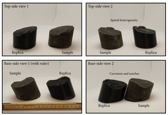
Figure 5.
Comparison of a 3D printed replica and the original drill core sample. Such a comparison was implemented as a first quality indicator for the equivalence of the dimensions and volume.
Models implementing both GCP types featured similar root mean square errors (RMSEs). Though not impacting accuracy and precision, the proprietary 12 bit Metashape markers generally required more manual fine-tuning and quality assurance for correct marker placement than the ArUco markers. RMSE increase (several orders of magnitude; e.g., both DH4-568a and b), volume overestimates (e.g., DH4-568a, +40%) and underestimates (e.g., DH4-568b, −25%) are associated with fewer GCPs and non-object-surrounding configurations, which is likely a result of insufficient coordinate truthing around the object.
Figure 6 outlines the fits observed between volumes, masses, and densities as obtained from the geotechnical immersion in fluid and photogrammetric methods. Mean deviations between the two methods are at per mille levels, with the biggest per-sample volumetric and bulk density deviation observed for DH4-591. All other samples are found to be within a 1% difference interval, supporting the observed equivalence between both methods.
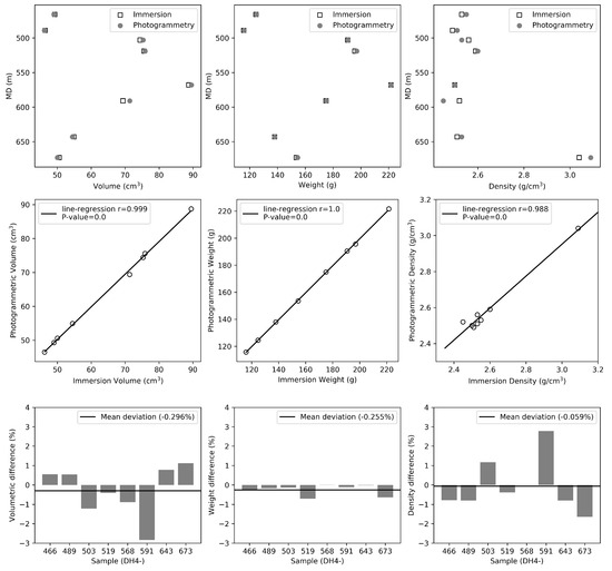
Figure 6.
Volumes, masses, and bulk densities as derived from the immersion in fluid and photogrammetric methods.
3.2. Core Characterisation and Alignment
DH4-487.5 was used to highlight the capability of using unwrapped cores for structural analyses and sedimentological core characterisation.
A simplified interpretation of both structural (e.g., fractures, deformation bands) and sedimentary (e.g., lamina–laminaset facies) features is shown in Figure 7, and illustrates the undistorted orthophotographic projection of the six fragments (DH4-487.5a–f) reconstructed into the composite DCM DH4-487.5 that covers the interval from 487.45 to 487.53 m MD (Figure 8). Though relatively heavily fractured, this interval was chosen to illustrate the alignment of (unwrapped) DCMs with televiewer data.
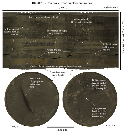
Figure 7.
Top, side and base of composite DCM DH4-487.5 with labelling of the main observed structure-sedimentological features.
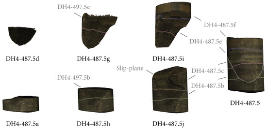
Figure 8.
Various stages of composite DCM reconstruction. DH4-487.5i and j complement each other across a slip surface and fracture to form DH4-487.5. The slip surface and fracture align with an anomaly observed in televiewer data at the corresponding interval (see Figure 9).
In particular, apart from natural fractures, fine details like sedimentary faces related to subtle differences in grain size populations can be easily recognised, and analysed in their 3D development. Along the same line, drilling- and decompaction-related artefacts (i.e., bedding-parallel and -perpendicular fractures/cracks, torque striations) can be distinguished based on their surface features, and cross-cut and abutting relationships. Cut-off angles are clearly preserved thanks to the 2D unwrapping. Other heterogeneous textural features can be readily observed. These are related to local changes in mineralogical composition, grain size distributions, and relationships with the host rock (e.g., bioturbation, diagenetic products).
The drilling-induced and pre-existing fractures, with dimensions varying from hairline (ca. 0.1 mm) up to ca. 2 mm, are indicated in Figure 7. These have been used to pinpoint the alignment between the 2D orthoprojection and the corresponding televiewer data interval (Figure 9). With the exception of the latter, most artificial fractures appear sub-parallel to the bedding, and not visible in televiewer data, being most likely developed during core retrieval (decompaction cracks) and/or related to the rotatory movement of the corer (drill biscuits). The sole (sinusoid) anomaly observed in televiewer data appears to correspond with the (likely) pre-existing, natural fracture, which also features a slip-plane as indicated by shiny surfaces on both DH4-487.5i and j (Figure 8). Through the alignment of both sinusoids, the slip-plane and DCM were calibrated with real-world bearings and the in situ orientation, whereas the calibrated depth of the cored interval was deduced.
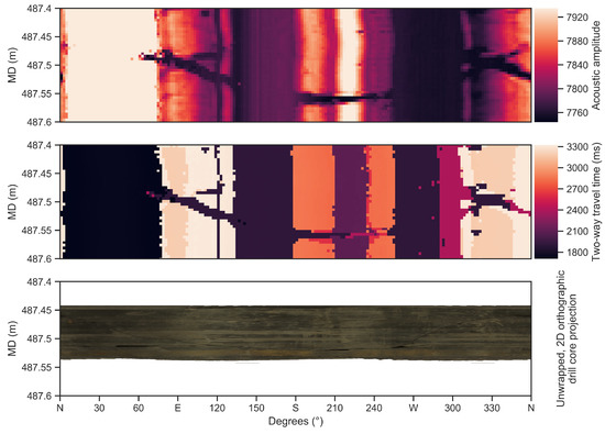
Figure 9.
Alignment and matching of an unwrapped core (DH4, 487.5 m MD; Figure 7) with transit time and amplitude acoustic televiewer data. The anomaly observed in both transit time and amplitude data at the 487.45-487.53 m interval corresponds to a fracture and slip surface observed at roughly the same interval in composite core DH4-487.5 (Figure 8).
4. Discussion
4.1. Feature Alignment during SfM
In some cases, manual processing and changes to Metashape default settings were sporadically needed during SfM processing. The observed alignment failures can be subdivided into two groups. The first contains cases without sufficient image overlap, which can be corrected by re-visiting the photographic acquisition step for additional data. Aided by imaging the samples in a second side-view orientation, this provides additional angles of overlap and solved most cases.
The second group failed to align due to various technical reasons, either related to processing settings and/or to changes in acquisition parameters. To enhance processing rates, for instance, Metashape features several algorithms that pre-select image pairs for matching. While ensuring decreased processing times under normal use, these algorithms may lead to the failure of alignment upon processing of small and texture-similar samples. By disabling the generic and reference pre-selection modules, all images are compared against the entire data set at full resolutions (versus downscaling of images and order-wise comparison ), resulting in improved alignment for this specific use-case [40].
In other cases, image-selections had to be re-aligned manually in a two-step alignment process. Here, the selective alignment of GCP-containing images proofed useful as an alignment-anchor/tie point for the remaining images, allowing for the alignment of images with different sets of acquisition parameters (e.g., different focal lengths). The use of calibrations aids during the photography step of one of the orientations further improved the alignment of samples. The extra key points, which are directly linked to a pose, prevented misalignments that arise from the texture-similar (i.e., mostly mud-dominated) samples. The alignment of smaller samples benefited the most from such corrections, which may be related to the lower number of key points associated with them.
4.2. Volume Assessment and Error-Contributing Factors
Differences between the immersion in fluid and photogrammetric methods may arise due to several factors. However, volumetric errors do not appear related to the use of a particular software suite, with both open-source (e.g., Blender) and commercial (e.g., Metashape) packages resulting in near-identical outcomes (i.e., up to at least the third digit). Neither are differences observed to arise from the implementation of different GCP workflows, which assign marker coordinates prior to the processing stage. While not having an impact on accuracy and precision, the use of ArUco markers in the Python-based workflow does significantly cut the amount of time by making manual marker calibration and assignment redundant, as opposed to the Metashape 12-bit marker workflow where manual intervention was a necessity.
Disabling of several GCPs during pre-processing led to more significant differences in volumes and spatial accuracy. A low number of GCPs put on a single line on one side of the sample, for example, resulted in anomalous DCM volumes deviating either positively or negatively (Table 2). As soon as a minimum threshold of GCPs in object-centric placement is passed, the net accuracy and precision gain of introducing more GCPs diminishes, as seen by the RMSE and volume differences between DH4-568, DH4-568a, b, and d. Similar findings have been observed during supra-metre scale studies (e.g., [46,47]), which indicate that horizontal and vertical accuracy increases as the GCP-count increases and the distribution is optimised.
Table 2.
Overview of volumes, masses, and bulk densities as derived from the photogrammetric (p) and geotechnical immersion in fluid (I) methods. Refer to the main text for detailed procedures, and see Figure 6 for further correlations.
More crucial than the RMSE error of the GCPs is the (hypothesised) equivalence between geotechnical and photogrammetric volume estimates. With mean relative volume differences between both methods at per mille levels, the use of photogrammetry appears suitable as a cost-effective alternative to traditional, sample-altering methods like the immersion in fluid procedure. The near-outlier DH4-591 does indeed exceed the 1% mark with almost 3% deviation or slightly less than 2 cm3 in terms of absolute volume (versus a sample volume of approximately 70 cm3). As both procedures determine volume indirectly, the difference may be the result of errors in either method, as well as due to the samples physically changing over time. The extended time between cold-storage, photogrammetric acquisition, and the immersion in fluid tests may have led to swelling and/or shrinkage, caused by drying and/or wetting resulting from changes in environmental conditions. This phenomenon has previously been reported during a permeability assessment on samples from the same borehole [32]. Furthermore, samples may have been damaged during for example storage, transport, and immersion, with each step increasing the likelihood thereof. Although masses measured prior to photogrammetry and the immersion in fluid tests indicate no significant differences, different volumetric differences are observed during post-waxing determination of the volumes. The latter narrows down the volumetric difference to 1.48% (i.e., half the original difference), with re-assessment of the post-waxing volumes (DH4-591w) through the photogrammetric method and immersion in fluid method yielding 73.2 cm3 (+1.9 cm3) and 74.3 cm3 (+4.48 cm3), respectively.
Upon retrieval, re-examination of the wax-coated sample indicated insufficient waxing for parts of the sample, directly exposing the drill core to fluids during immersion. In the presence of a (micro-)fracture network, this may be sufficient for fluids to enter the drill core sample and impact the outcome of the measurement. Though likely only a minor factor, migration of wax into the network may have further contributed to the observed difference, and is indirectly supported by the pre/post-waxing volume difference changes attributed to the wax-coating itself.
The overall equivalence derived from all eight samples remains statistically significant, with the mean deviation between both techniques coming down to 0.059%. Furthermore, the method appears indifferent to the symmetricity and size of samples, making small-scale, close-up photogrammetry suitable for both volume and bulk density calculations. Finally, the immersion in fluid method requires substantial more physical handling and processing of the sample than the photogrammetric method, increasing the likelihood of (accidental) damage and human error. For higher numbers of samples, this physical aspect further limits the cost- and time-benefits made possible through the (semi-)automation offered by the photogrammetric method.
Thus, this work shows that the same principles of bulk density analysis and quantification of e.g., soil aggregates (e.g., [48]) can indeed be used to accurately determine bulk densities of drill core and other geological samples. The benefit of not being destructive or sample-altering is highly beneficial, and shows that the photogrammetric method is a suitable option for the calibration of the Longyearbyen CO2 Lab density wireline logs. Having been stored in a semi-continuously frozen setting since being drilled, the properties of the well-cemented drill core samples obtained from the Longyearbyen CO2 Lab are unlikely to have changed substantially over time, and are likely closest to the in situ conditions. As such, the use of photogrammetry-derived bulk densities is likely to be extended to selected intervals covered by the available wireline logging, providing a cost- and time-effective alternative to traditional methods and an efficient means to obtaining quantitative bulk density data in-house using off-the-shelf components.
4.3. 3D Image Analysis and Characterisation
Like virtual outcrop models (VOMs), we have shown that DCMs can be used to generate pseudo-cross-sectional profiles that are amenable to qualitative and quantitative, image-based analyses. Digital characterisation techniques originally developed for VOMs are therefore applicable to DCMs as well, allowing for the easy extraction, elucidation and transfer of geological information (e.g., [3,49]).
DCM profiles are readily generated through the “unwrapping” of core textures projected on a cylindrical mesh, resulting in 2D orthographic images of the core sides (i.e., top, side, base). Though this procedure is relatively straight forward, artefacts in the pseudo-cross-section arise when the projection-mesh and DCM are too far apart (Figure 7). This divergence in position mostly stems from differences in shape, and can be minimalised by better tuning the shape of the projection-mesh to the DCM. However, the latter leads to altering perspectives of the unwrapped texture, and the masking of non-parallel sections may therefore yield better results, at least when the circumference profile is concerned.
In Figure 7, for instance, the aforementioned mis-projections are visible at the top and bottom edges, where jagging, repetitions, and other projection-anomalies occur. If unnoticed, such anomalies are likely to interfere with the correct interpretation. Especially when used in conjunction with automated structural and material analyses (e.g., automated image processing), this (current) limitation should be kept in mind. Similar anomalies arise from the stitching of multiple fragments, as indicated in Figure 7. Here they are a likely result of the ill-lit stitching space between individual core fragments, which is a side effect of the reconstruction of composite cores from fragments.
The ability to reconstruct cores from individual core fragments allows for the reconstruction of highly fractured intervals into composite DCMs (Figure 8), which can theoretically be extended (digitally) to encompass all available core material for a given borehole. The two procedures summarised here strongly differ in efficiency and automation potential. Currently, closely aligning fragments during the photographic acquisition step is found to be more effective, especially considering that manual reconstruction and alignment of segments using 3D software is far more time-consuming. A significant increase in efficiency is expected when implementing novel alignment methods and techniques within the latter. The potential of object-reassembly algorithms (e.g., [50,51]) underlines this expectation, and it is likely to result in a fully automated add-on to the current workflow. Until then, object-reassembly effectively takes place during the photographic acquisition step. By imaging interfaces of connected segments, enough keypoints and overlap between fragments are afforded to allow for SfM processing to reconstruct composite models within an accurate coordinate system. Through the latter procedure, the 487.45–487.53 m MD interval of DH4 was reconstructed. This interval was selected due to a clear sinusoid structural pattern visible in acoustic televiewer data (Figure 9), potentially allowing for the determination of the in situ core orientation and depth if also observed in the corresponding pseudo-cross-sections of the DCM.
Unwrapped core textures can be treated as directly correlatable to optical televiewer data from the same depth. As a result, related features may be directly compared to borehole-wall imagery, and used to both correct orientation and depth of the core. During such a re-alignment, it is important to note that discrepancies between logged core intervals and televiewer data may exist, resulting from cable stretch, irregular tool movement (which may further adversely impact the data), misalignment and loss of drill core samples [52]. In addition, a limited feature and signal count in televiewer data is expected when dealing with flay-lying, homogeneous units.
Such a setting is partly encountered in our case study targeting the shale-rich, Late-Jurassic Agardhfjellet Formation, which makes up most of the interval for which televiewer data is available. The initial comparison between (boxed) drill cores and televiewer data indicated the damage sampling, poor handling and sample degradation can lead to. Most anomalies found in televiewer data pertain to previously, heavily sampled core intervals, or were fully pulverised and smashed up as a result of wear and tear through operational activities. Furthermore, discrepancies were observed between (boxed) core samples and the televiewer data, with mismatching structures (e.g., presence/absence of fractures) documented at similar depth. In general, these findings are quite likely the result of less-than-optimal televiewer data, and the impact of such features as breakouts and faulty tool orientation. Additionally, units featuring nicely dipping marker beds (e.g., coal seams in the Helvetiafjellet Formation), are beyond the televiewer-logged interval, preventing comparison. The applicability of the proposed protocol is therefore likely to increase for more favourable settings that include steeper dipping depositional angles and more geological heterogeneity. In such cases, orientations may be deduced based on structural and sedimentary facies alone.
Nonetheless, the feasibility of the technique (even under far from optimal conditions) has been successfully demonstrated through the analysis of sample DH4-487.5. Besides confirming orientation and depth, the alignment also shows which fractures are present in situ, and which are likely drilling-induced. This provides a valuable aid during fracture characterisation, in addition to being an efficient way of visualising stratigraphic-sedimentary details.
The combination of digital reconstruction and positioning allows for the in situ orientation to easily be extrapolated to a larger section of the core, which in turn may be used to determine the geometrical relationships among structures, tectonic stress and kinematic history [53]. As neither proprietary hardware nor software is needed, the photogrammetry-based procedure lowers the requirements with which this can be done compared to other standard and widely used core-orienting techniques [53,54]. As a follow-up (currently) beyond the capabilities of the Longyearbyen CO2 Lab, it would be interesting to compare optical televiewer data with the reconstructed, directly correlatable televiewer analogue derived from unwrapped cores.
4.4. Future Applications
The applicability of the proposed workflow allows for a straightforward application of SfM photogrammetry to geological hand specimens. Beyond drill core samples, potential uses are, in particular, envisaged for the characterisation and (digital) documentation of delicate and dangerous (e.g., radioactive) materials prior to destructive testing, in-field bulk density assessments, and the establishment of readily accessible DCM repositories (including geoscientific metadata) that guarantee enhanced scientific repeatability. As such, we foresee the potential of this method for the digitisation of ice and permafrost cores in addition to soil, mineral, and rock samples.
The digitisation and (digital) storage of drill core samples is complementary to existing physical and photographic sample archives, providing capabilities to remotely access and analyse 3D model. However, like with physical storage, several recommendations are needed to prevent the loss of data, to ensure the access to the archive, and to validate results. Due to similarity in object types and scales, we base these recommendations on the EAC guidelines for best practices in European archaeological archiving [55]:
- All scientific digitisation projects must result in a secure, stable, ordered, and accessible archive, featuring digital backup strategies and updated, (semi-)permanent storage solutions.
- Standards and procedures for the creation, selection, management, compilation and transfer of the archive must be agreed upon in the design stage, and each procedure must be fully documented.
- The entire archive must be compiled in such a way to ensure the preservation of relationships between elements and to facilitate access to all parts in the future. This also includes the linked storage of such related and derived data as interpretations and subsequent processing.
- Where possible, physical and digital sample storage should be in the same place, or at least stored through association, to prevent red tape from being in the way of access.
- Finally, a digitisation project is only completed after the archive has been transferred to a recognised repository, and is fully accessible for consultation.
Beyond the archival value, digital sample repositories allow for the use of big data tools (e.g., machine learning), which may extend the use of digital samples to methods that are currently limited to 2D images (e.g., optical mineralogical characterisation [56,57]), turning such repositories into actual digital laboratories.
To lay the foundation for an accessible digital drill core repository on Svalbard, all generated models have been integrated into the Svalbox database, which is a showcase geoscientific database for high Arctic teaching and research [58] conforming the recommendations outlined above. Other examples of such geoscientific databases include SafariDB [59] and eRocK [60], which may be expanded to include digital rock samples as well.
5. Conclusions
Following optimisation and automatisation of the described workflow, high resolution DCMs can be inexpensively obtained within short time frames, and provide a foundation for a combined analogue-digital characterisation. The use of DCMs in volume calculations provides a non-destructive, cost- and time-effective means of characterisation compared to traditional methods such as immersion in fluid. The photogrammetric method results in equal to better volume estimates and thereof-derived bulk densities. Furthermore, unwrapping cores by using 3D software tools allows for unprecedented analytical opportunities, ranging from accurate structural (e.g., fracture) and sedimentological (e.g., sedimentary facies) characterisation to the virtual reconstruction and televiewer-aided re-orientation of drill core segments and fragments. Re-alignment is enabled through comparison of the 2D orthographic depiction of the core edge with borehole imagery (televiewer) data of the same interval. These benefits, in combination with the inherent value of having cores digitally stored and readily accessible long after the destruction or loss of the physical sample, exceeds any argument against making DCMs available as part of the publication and archival process. Finally, as the methods and applications outlined in this contribution are not only applicable to drill core samples, we recommend the same procedure to be tested for other types of geological samples, including degradable and dangerous ice/hydrate and sediment cores.
Author Contributions
Conceptualisation, P.B., T.B. and K.S.; Data curation, P.B. and K.S.; Formal analysis, P.B., K.O. and K.S.; Funding acquisition, E.S. and K.S.; Investigation, P.B.; Methodology, P.B. and T.B.; Project administration, P.B.; Resources, P.B., T.B., K.O., J.P., E.S. and K.S.; Software, P.B.; Supervision, K.O., J.P., E.S. and K.S.; Validation, P.B., J.P., E.S. and K.S.; Visualisation, P.B.; Writing-original draft, P.B., T.B., K.O., J.P., E.S. and K.S.; Writing—review and editing, P.B., T.B., and K.S. All authors have read and agree to the published version of the manuscript.
Funding
This research was funded by the Norwegian CCS Research Centre (NCCS), supported by industry partners and Norwegian Research Council grant 257579, the Research Centre for Arctic Petroleum Exploration (ARCEx), supported by industry partners and Norwegian Research Council grant 228107, and the University of the Arctic (UArctic).
Acknowledgments
We sincerely appreciate the UNIS CO2 Lab (http://co2-ccs.unis.no) for access to the CO2 research borehole data from onshore Svalbard. We thank Kristine Halvorsen, Jenny Robinson, and Geir Åsli for conducting the geotechnical bulk volume and density measurements. UNIS further acknowledges the academic licenses of Petrel, the Blueback Toolbox, and Metashape provided by Schlumberger, Cegal, and Agisoft, respectively. Finally, we thank three anonymous reviewers and editor Datura Yang for their constructive feedback.
Conflicts of Interest
The authors declare no conflict of interest. The funders had no role in the design of the study; in the collection, analyses, or interpretation of data; in the writing of the manuscript, or in the decision to publish the results.
Abbreviations
The following abbreviations are used in this manuscript:
| CC(U)S | carbon capture, (use) and storage |
| DCM | digital (drill) core model |
| GCP | ground control point |
| MD | measured depth |
| RMSE | root mean square error |
| SfM | structure-from-motion |
| VOM | virtual outcrop model |
References
- Westoby, M.J.; Brasington, J.; Glasser, N.F.; Hambrey, M.J.; Reynolds, J.M. ’Structure-from-Motion’ photogrammetry: A low-cost, effective tool for geoscience applications. Geomorphology 2012, 179, 300–314. [Google Scholar] [CrossRef]
- Carrivick, J.; Smith, M.; Quincey, D. Structure from Motion in the Geosciences; Wiley-Blackwell: Hoboken, NJ, USA, 2016; p. 197. [Google Scholar] [CrossRef]
- Pringle, J.K.; Howell, J.A.; Hodgetts, D.; Westerman, A.R.; Hodgson, D.M. Virtual outcrop models of petroleum reservoir analogues: A review of the current state-of-the-art. First Break 2006, 24, 33–42. [Google Scholar] [CrossRef]
- Yilmaz, H.M. Close range photogrammetry in volume computing. Exp. Tech. 2010, 34, 48–54. [Google Scholar] [CrossRef]
- Hasiuk, F. Making things geological: 3-D printing in the geosciences. GSA Today 2014, 24, 28–29. [Google Scholar] [CrossRef]
- Wajs, J. Research on surveying technology applied for DTM modelling and volume computation in open pit mines. Min. Sci. 2015, 22, 75–83. [Google Scholar] [CrossRef]
- Banu, T.P.; Borlea, G.F.; Banu, C. The Use of Drones in Forestry. J. Environ. Sci. Eng. B 2016, 5, 557–562. [Google Scholar] [CrossRef]
- Vallet, J.; Gruber, U.; Dufour, F. Photogrammetric avalanche volume measurements at Vallée de la Sionne, Switzerland. Ann. Glaciol. 2001, 32, 141–146. [Google Scholar] [CrossRef]
- Cardenal, J.; Mata, E.; Perez-Garcia, J.; Delgado, J.; Andez, A.; Gonzalez, A.; Diaz-de Teran, J. Close range digital photogrammetry techniques applied to landslide monitoring. Int. Arch. Photogramm. Remote Sens. Spat. Inf. Sci. 2008, 37, 235–240. [Google Scholar]
- Grazioso, S.; Caporaso, T.; Selvaggio, M.; Panariello, D.; Ruggiero, R.; Di Gironimo, G. Using photogrammetric 3D body reconstruction for the design of patient–tailored assistive devices. In Proceedings of the 2019 II Workshop on Metrology for Industry 4.0 and IoT (MetroInd4.0 and IoT). Institute of Electrical and Electronics Engineers (IEEE), Naples, Italy, 4–6 June 2019; pp. 240–242. [Google Scholar] [CrossRef]
- Mitchell, J.; Chandrasekera, T.C.; Holland, D.J.; Gladden, L.F.; Fordham, E.J. Magnetic resonance imaging in laboratory petrophysical core analysis. Phys. Rep. 2013, 526, 165–225. [Google Scholar] [CrossRef]
- Van Stappen, J.F.; Meftah, R.; Boone, M.A.; Bultreys, T.; De Kock, T.; Blykers, B.K.; Senger, K.; Olaussen, S.; Cnudde, V. In Situ Triaxial Testing to Determine Fracture Permeability and Aperture Distribution for CO2 Sequestration in Svalbard, Norway. Environ. Sci. Technol. 2018, 52, 4546–4554. [Google Scholar] [CrossRef] [PubMed]
- Tangelder, J.W.; Ermes, P.; Vosselman, G.; van den Heuvel, F.A. CAD-based photogrammetry for reverse engineering of industrial installations. Comput.-Aided Civ. Infrastruct. Eng. 2003, 18, 264–274. [Google Scholar] [CrossRef]
- Remondino, F. Heritage recording and 3D modeling with photogrammetry and 3D scanning. Remote Sens. 2011, 3, 1104–1138. [Google Scholar] [CrossRef]
- Falkingham, P.L. Acquisition of high resolution three-dimensional models using free, open-source, photogrammetric software. Palaeontol. Electron. 2012, 15. [Google Scholar] [CrossRef]
- Eulitz, M.; Reiss, G. 3D reconstruction of SEM images by use of optical photogrammetry software. J. Struct. Biol. 2015, 191, 190–196. [Google Scholar] [CrossRef]
- Casini, G.; Hunt, D.W.; Monsen, E.; Bounaim, A. Fracture characterization and modeling from virtual outcrops. AAPG Bull. 2016, 100, 41–61. [Google Scholar] [CrossRef]
- Enge, H.D.; Buckley, S.J.; Rotevatn, A.; Howell, J.A. From outcrop to reservoir simulation model: Workflow and procedures. Geosphere 2007, 3, 469–490. [Google Scholar] [CrossRef]
- Eide, C.H.; Schofield, N.; Lecomte, I.; Buckley, S.J.; Howell, J.A. Seismic interpretation of sill complexes in sedimentary basins: Implications for the sub-sill imaging problem. J. Geol. Soc. 2018, 175, 193–209. [Google Scholar] [CrossRef]
- Bellian, J.; Kerans, C.; Jennette, D. Digital Outcrop Models: Applications of Terrestrial Scanning Lidar Technology in Stratigraphic Modeling. J. Sediment. Res. 2005, 75, 166–176. [Google Scholar] [CrossRef]
- Smith, H.; Bohloli, B.; Skurtveit, E.; Mondol, N.H. Engineering parameters of draupne shale—Fracture characterization and integration with mechanical data. In Proceedings of the 6th EAGE Shale Workshop, Bordeaux, France, 29 April–2 May 2019. [Google Scholar] [CrossRef]
- McGinnis, M.J.; Pessiki, S.; Turker, H. Application of three-dimensional digital image correlation to the core-drilling method. Exp. Mech. 2005, 45, 359–367. [Google Scholar] [CrossRef]
- Ren, W.; Kou, X.; Ling, H. Application of digital close-range photogrammetry in deformation measurement of model test. Yanshilixue Yu Gongcheng Xuebao/Chin. J. Rock Mech. Eng. 2004, 23, 436–440. [Google Scholar]
- Maas, H.G.; Hampel, U. Programmetric techniques in civil engineering material testing and structure monitoring. Photogramm. Eng. Remote Sens. 2006, 72, 39–45. [Google Scholar] [CrossRef]
- Benton, D.J.; Iverson, S.R.; Martin, L.A.; Johnson, J.C.; Raffaldi, M.J. Volumetric measurement of rock movement using photogrammetry. Int. J. Min. Sci. Technol. 2016, 26, 123–130. [Google Scholar] [CrossRef] [PubMed][Green Version]
- De Paor, D.G. Virtual Rocks. GSA Today 2016, 26, 4–11. [Google Scholar] [CrossRef]
- Mallison, H.; Wings, O. Photogrammetry in paleontology—A practical guide. J. Paleontol. Tech. 2014, 12, 1–31. [Google Scholar]
- Dombroski, C.E.; Balsdon, M.E.; Froats, A. The use of a low cost 3D scanning and printing tool in the manufacture of custom-made foot orthoses: A preliminary study. BMC Res. Notes 2014, 7, 443. [Google Scholar] [CrossRef]
- Olaussen, S.; Senger, K.; Braathen, A.; Grundvåg, S.A.; Mørk, A. You learn as long as you drill; research synthetis from the Longyearbyen CO2 Laboratory, Svalbard, Norway. Nor. J. Geol. 2019. [Google Scholar] [CrossRef]
- Braathen, A.; Bælum, K.; Christiansen, H.; Dahl, T.; Eiken, O.; Elvebakk, H.; Hansen, F.; Hanssen, T.; Jochmann, M.; Johansen, T.; et al. The Longyearbyen CO2 Lab of Svalbard, Norway—Initial assessment of the geological conditions for CO2 sequestration. Nor. J. Geol. 2012, 92, 353–376. [Google Scholar]
- Larsen, L. Analyses of Sept. 2011 Upper Zone Injection and Falloff Data from DH6 and Interference Data from DH5; Technical Report; UNIS CO2 Lab: Longyearbyen, Svalbard, 2012. [Google Scholar]
- Magnabosco, C.; Braathen, A.; Ogata, K. Permeability model of tight reservoir sandstones combining core-plug and Miniperm analysis of drillcore; Longyearbyen CO2 Lab, Svalbard. Nor. J. Geol. 2014, 94, 189–200. [Google Scholar]
- Ogata, K.; Senger, K.; Braathen, A.; Tveranger, J.; Olaussen, S. Fracture systems and mesoscale structural patterns in the siliciclastic Mesozoic reservoir-caprock succession of the Longyearbyen CO2 Lab project: Implications for geological CO2 sequestration in Central Spitsbergen, Svalbard. Nor. J. Geol. 2014, 94, 121–154. [Google Scholar]
- Bohloli, B.; Skurtveit, E.; Grande, L.; Titlestad, G.O.; Børresen, M.H.; Johnsen, Ø.; Braathen, A.; Braathen, A. Evaluation of reservoir and cap-rock integrity for the longyearbyen CO2 storage pilot based on laboratory experiments and injection tests. Nor. J. Geol. 2014, 94, 171–187. [Google Scholar]
- Elvebakk, H. Results of borehole logging in well LYB CO2, Dh4 of 2009, Longyearbyen, Svalbard. Technical Report; NGU: Trondheim, Norway, 2010. [Google Scholar]
- Lubrano-Lavadera, P.; Senger, K.; Lecomte, I.; Mulrooney, M.J.; Kühn, D. Seismic modelling of metre-scale normal faults at a reservoir-cap rock interface in Central Spitsbergen, Svalbard: Implications for CO2 storage. Nor. J. Geol. 2019. [Google Scholar] [CrossRef]
- Koevoets, M.J.; Hammer, Ø.; Olaussen, S.; Senger, K.; Smelror, M.I. Integrating subsurface and outcrop data of the middle jurassic to lower cretaceous agardhfjellet formation in central spitsbergen. Nor. J. Geol. 2018, 98, 1–34. [Google Scholar] [CrossRef]
- Rismyhr, B.; Bjærke, T.; Olaussen, S.; Mulrooney, M.J.; Senger, K. Facies, palynostratigraphy and sequence stratigraphy of the Wilhelmøya Subgroup (Upper Triassic–Middle Jurassic) in western central Spitsbergen, Svalbard. Nor. J. Geol. 2019. [Google Scholar] [CrossRef]
- Mulrooney, M.J.; Larsen, L.; Van Stappen, J.; Rismyhr, B.; Senger, K.; Braathen, A.; Olaussen, S.; Mørk, M.B.E.; Ogata, K.; Cnudde, V. Fluid flow properties of the Wilhelmøya Subgroup, a potential unconventional CO2 storage unit in central Spitsbergen. Nor. J. Geol. 2018. [Google Scholar] [CrossRef]
- Agisoft. Agisoft Metashape User Manual Professional Edition, version 1.5; Agisoft LLC: St. Petersburg, Russia, 2018; p. 130. [Google Scholar]
- Garrido-Jurado, S.; Muñoz-Salinas, R.; Madrid-Cuevas, F.J.; Marín-Jiménez, M.J. Automatic generation and detection of highly reliable fiducial markers under occlusion. Pattern Recognit. 2014, 47, 2280–2292. [Google Scholar] [CrossRef]
- Bradski, G. The OpenCV Library. Dr. Dobbs J. Softw. Tools 2000, 25, 120–125. [Google Scholar] [CrossRef]
- Agisoft. Metashape Python Reference; Release 1.5.0; Agisoft LLC: St. Petersburg, Russia, 2018. [Google Scholar]
- Blender Foundation. Blender—A 3D Modelling and Rendering Package; Blender Foundation: Amsterdam, The Netherlands, 2019. [Google Scholar]
- ISO/TC 182 Geotechnics. ISO 17892-2:2014—Geotechnical Investigation and Testing—Laboratory Testing of Soil—Part 2: Determination of Bulk Density; Technical report; ISO: Geneva, Switzerland, 2014. [Google Scholar]
- Agüera-Vega, F.; Carvajal-Ramírez, F.; Martínez-Carricondo, P. Assessment of photogrammetric mapping accuracy based on variation ground control points number using unmanned aerial vehicle. Meas. J. Int. Meas. Confed. 2017, 98, 221–227. [Google Scholar] [CrossRef]
- Tonkin, T.N.; Midgley, N.G. Ground-control networks for image based surface reconstruction: An investigation of optimum survey designs using UAV derived imagery and structure-from-motion photogrammetry. Remote Sens. 2016, 8, 786. [Google Scholar] [CrossRef]
- Bauer, T.; Strauss, P.; Murer, E. A photogrammetric method for calculating soil bulk density§. J. Plant Nutr. Soil Sci. 2014, 177, 496–499. [Google Scholar] [CrossRef]
- Tavani, S.; Granado, P.; Corradetti, A.; Girundo, M.; Iannace, A.; Arbués, P.; Muñoz, J.A.; Mazzoli, S. Building a virtual outcrop, extracting geological information from it, and sharing the results in Google Earth via OpenPlot and Photoscan: An example from the Khaviz Anticline (Iran). Comput. Geosci. 2014, 63, 44–53. [Google Scholar] [CrossRef]
- Zhang, K.; Yu, W.; Manhein, M.; Waggenspack, W.; Li, X. 3D fragment reassembly using integrated template guidance and fracture-region matching. In Proceedings of the 2015 IEEE International Conference on Computer Vision (ICCV), Santiago, Chile, 7–13 December 2015. Technical Report. [Google Scholar] [CrossRef]
- Winkelbach, S.; Wahl, F.M. Pairwise matching of 3D fragments using cluster trees. Int. J. Comput. Vis. 2008, 78, 1–13. [Google Scholar] [CrossRef]
- Gwynn, X.; Brown, M.; Mohr, P. Combined use of traditional core logging and televiewer imaging for practical geotechnical data collection. In Proceedings of the 2013 International Symposium on Slope Stability in Open Pit Mining and Civil Engineering, Brisbane, QLD, Australia, 25–27 September 2013. [Google Scholar]
- Shigematsu, N.; Otsubo, M.; Fujimoto, K.; Tanaka, N. Orienting drill core using borehole-wall image correlation analysis. J. Struct. Geol. 2014, 67, 293–299. [Google Scholar] [CrossRef]
- Paulsen, T.S.; Jarrard, R.D.; Wilson, T.J. A simple method for orienting drill core by correlating features in whole-core scans and oriented borehole-wall imagery. J. Struct. Geol. 2002, 24, 1233–1238. [Google Scholar] [CrossRef]
- Perrin, K.; Brown, D.H.; Lange, G.; Bibby, D.; Carlsson, A.; Degraeve, A.; Kuna, M.; Larsson, Y.; Pàlsdottir, S.U.; Stoll-Tucker, B.; et al. A Standard and Guide To Best Practice for Archaeological Archiving in Europe; Europae Archaeologiae Consilium: Namur, Belgium, 2014; p. 66. [Google Scholar]
- Koch, P.H.; Lund, C.; Rosenkranz, J. Automated drill core mineralogical characterization method for texture classification and modal mineralogy estimation for geometallurgy. Miner. Eng. 2019, 136, 99–109. [Google Scholar] [CrossRef]
- Pérez-Barnuevo, L.; Lévesque, S.; Bazin, C. Automated recognition of drill core textures: A geometallurgical tool for mineral processing prediction. Miner. Eng. 2018, 118, 87–96. [Google Scholar] [CrossRef]
- Senger, K. Svalbox: A Geoscientific Database for High Arctic Teaching and Research. In Proceedings of the AAPG Annual Convention and Exhibition, San Antonio, TX, USA, 19–22 May 2019. [Google Scholar]
- Naumann, N.; Howell, J.A.; Buckley, S.J.; Ringdal, K.; Dolva, B.; Maxwell, G.; Chmielewska, M. New ways of sharing outcrop data: The SAFARI database and 3D web viewer. In Proceedings of the 3rd Virtual Geoscience Conference, Kingston, ON, Canada, 22–24 August 2018. [Google Scholar]
- Cawood, A.; Bond, C. eRock: An Open-Access Repository of Virtual Outcrops for Geoscience Education. GSA Today 2019, 29, 36–37. [Google Scholar] [CrossRef]
Sample Availability: Raw and processed resources (i.e., photos, marker pages, marker distances, Metashape projects, and models) are available through the Svalbox repository (svalbox.no) upon request, following the UNIS CO2 Lab guidelines on data accessibility. |
© 2020 by the authors. Licensee MDPI, Basel, Switzerland. This article is an open access article distributed under the terms and conditions of the Creative Commons Attribution (CC BY) license (http://creativecommons.org/licenses/by/4.0/).