Abstract
The selection of an appropriate global gravity field model and refinement method can effectively improve the accuracy of the refined regional geoid model in a certain research area. We analyzed the accuracy of Experimental Geopotential Model (XGM2016) based on the GPS-leveling data and the modification parameters of the global mean square errors in the KTH geoid refinement in Jilin Province, China. The regional geoid was refined based on Earth Gravitational Model (EGM2008) and XGM2016 using both the Helmert condensation method with an RCR procedure and the KTH method. A comparison of the original two gravity field models to the GPS-leveling benchmarks showed that the accuracies of XGM2016 and EGM2008 in the plain area of Jilin Province are similar with a standard deviation (STD) of 5.8 cm, whereas the accuracy of EGM2008 in the high mountainous area is 1.4 cm better than that of XGM2016, which may be attributed to its low resolution. The modification parameters between the two gravity field models showed that the coefficient error of XGM2016 model was lower than that of EGM2008 for the same degree of expansion. The different modification limits and integral radii may produce a centimeter level difference in global mean square error, while the influence of the truncation error caused by the integral was at the millimeter level. The terrestrial gravity data error accounted for the majority of the global mean square error. The optimal least squares modification obtained the minimum global mean square error, and the global mean square error calculated based on XGM2016 model was reduced by about 1~3 cm compared with EGM2008. The refined geoid based on the two gravity field models indicated that both KTH and RCR method can effectively improve the STD of the geoid model from about six to three centimeters. The refined accuracy of EGM2008 model using RCR and KTH methods is slightly better than that of XGM2016 model in the plain and high mountain areas after seven-parameter fitting. EGM2008 based on the KTH method was the most precise at ± 2.0 cm in the plain area and ± 2.4 cm in the mountainous area. Generally, for the refined geoid based on the two Earth gravity models, KTH produced results similar to RCR in the plain area, and had relatively better performance for the mountainous area where terrestrial gravity data is sparse and unevenly distributed.
1. Introduction
A geoid is a gravity equipotential surface model that aligns with mean sea level and extends through the continents; it is used as a reference for heights in vertical datums [1]. The factors affecting geoid refinement are terrestrial gravity data, refinement methods, and gravity field models. The acquisition of terrestrial gravity data is considerably affected by the terrain, and the resolution improvement of terrestrial gravity data is time-consuming and costly, which means that the selection of an appropriate refining method and global gravity field model is necessary for local geoid refinement.
The most widely used geoid refinement method is the remove-compute-restore (RCR) technique [2], which uses the global gravity field model as a long-wavelength term and performs Stokes integration on the residual gravity anomaly to obtain high-frequency signals that are missing from the gravity field model. It should be noted that the influence of topography is taken into account in the computation of residual gravity anomalies [3]. The RCR method has been widely applied to the refinement of geoids, such as in Turkey [4], Canada [5], Australia [6], the United States [7], and Japan [8]. Given that the RCR method does not make full use of the long-wavelength information provided by the gravity field model during the refinement process, the Royal Institute of Technology (KTH) method proposed by Sjöberg modifies the Stokes kernel functions targeted at a minimum value of the global mean square error [9,10]. The terrestrial gravity data error, gravity field model, and its truncation error are optimally correlated in KTH, and therefore the determination of the least-squares parameters is a key issue for KTH geoid refinement [11,12]. Three methods for the determination of the least-squares parameters were summarized by Sjöberg, including biased least-squares modification (BLSM) [13], unbiased least-squares modification (ULSM) [14], and optimum least-squares modification (OLSM) [15]. The KTH method maximizes the advantage of the gravity field model in medium and long-wavelength sub-items, reduces the truncation error caused by the maximum order of the model, and has produced high accuracy geoid models in many countries, such as Sweden [16], Baltic countries [17,18], Iran [19], Tanzania [20], Sudan [21], Turkey [22], and Uganda [23].
EGM2008 is complete to spherical harmonic d/o 2159 and contains additional coefficients extending to degree 2190 and order 2159 [24]. Due to its high global applicability, EGM2008 has been widely used for geoid refinement [8,16,25,26]. The NGA announced that a new global gravity field model, EGM2020, is under development and will maintain the same resolution, but with superior accuracy as compared to EGM2008 [27]. Prior to releasing the latter, the XGM2016 model was developed and released as a preliminary result of the EGM2020. XGM2016 is a low-degree version of EGM2020 with spherical harmonic coefficients complete to d/o 719, which has been proven to be more accurate than EGM2008 over land and ocean [28].
The quality of regional geoid refinement may be highly impacted by the input data (the density and accuracy of the terrestrial gravity data and GPS-leveling data) and the refinement method [29]. Yildiz used the RCR and KTH methods to refine the regional geoid in the mostly flat Auvergne test area with densely distributed terrestrial gravity data. The results of the two methods produced large differences in the high mountainous areas that occupied a few portions of the study area [30]. Abbak selected the mountainous area of central Turkey as the experimental area with sparse terrestrial gravity data and a single GPS leveling route; the results showed that the KTH method was significantly better than the RCR method [22]. Abdalla conducted the same experiment in the Khartoum state of Sudan with the blank boundary of the area filled by EGM2008; the final results were produced at the decimeter level [31], which may be attributed to the poor accuracy of the original EGM2008 model in the area.
In this paper, we aimed to verify the applicability of regional geoid refinement when the EGM2008 and XGM2016 models were combined with the Helmert condensation method following an RCR procedure and KTH methods. The effects of the modification parameters on the global mean square error and the modified Stokes kernel function were analyzed using the KTH method to compare the accuracy difference between XGM2016 and EGM2008. Two aspects were considered for the selection of Jilin Province in Northeastern China as the experimental area. First, the KTH method has rarely been applied in China. Second, the terrain in Jilin Province intensely varies, including the plains in the west and the high mountains in the east, which is suitable for the analysis and comparison of geoid refinement accuracy using different models and methods in plain and mountainous areas.
2. Data and Methods
2.1. Study Area and Data
Jilin Province is located in the Songhua and Liao river basins in Northeastern China, with a total area of about 187,400 km2. The topography of Jilin Province is relatively complex and the height difference between the east and the west is more than 2400 m. This paper chose the western plain (Area A) and the eastern mountainous region (Area B) as experimental areas (Figure 1). Area A has a flat terrain with an average elevation of about 190 m and a height difference of about 100 m. Area B has a more complex topography, with an average elevation of about 700 m and a height difference of about 1300 m.
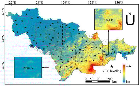
Figure 1.
Distribution of GPS-leveling benchmarks and gravity data in Jilin Province, China.
EGM2008 and XGM2016 were both tested in agreement with GPS-leveling data in the study area. EGM2008 was developed and released by the National Geospatial-Intelligence Agency (NGA), combining Gravity Recovery and Climate Experiment (GRACE) satellite gravity data and terrestrial gravity data with a model resolution of 5‘ x 5‘ As an experimental model of EGM2020, the XGM2016 model uses for the long wavelength part the complete GOCE and nearly complete GRACE mission datasets combined with the global 15‘ x 15‘ grid gravity anomaly, including satellite altimetry data, terrestrial gravity data, airborne gravity and shipborne gravity data.
A total of about 9000 terrestrial gravity point values in the China Geodetic Coordinate System 2000 (CGCS2000) datum were used in geoid refinement of Areas A and B. The resolution of gravity data in Area A and its surrounding integral regions was about 2’, while the resolution was only 6’ for Area B. The free-air gravity anomaly of the discrete gravity point cannot be directly interpolated due to lack of sufficient smoothness, and the anomaly needs to be corrected using the Bouguer plate, and topographic and isostatic corrections. A gridding process was performed to obtain the isostatic gravity anomaly grid. The resolution of the corrected grid free-air gravity anomaly was 2.5’ x 2.5’. A Digital Elevation Model (DEM) is necessary for the reduction of the gravity data as well as for geoid computation; therefore, the Shuttle Radar Topography Mission (SRTM) with a resolution of 3” x 3” [32] was used in this study. The blank area of SRTM data on the ocean was filled by SRTM30_PLUS v8 data developed by the Scripps Institute of Oceanography, University of California San Diego (UCSD), which was released as a global DEM grid with resolution of 30” x 30” [33].
To compare and verify the accuracy of the RCR and KTH methods in the refinement of the geoid model in the study area, 81 high-precision GPS-leveling points distributed throughout the whole of Jilin Province were introduced, of which 15 each were evenly distributed in Areas A and B. The GPS-leveling points’ horizontal and vertical datum was the CGCS2000 national geodetic coordinate system and 1985 national elevation reference, respectively, with a horizontal accuracy of approximately ±1.0 cm and an elevation accuracy of approximately ± 1.0 cm.
2.2. KTH Method
2.2.1. Modification of Stokes’ Formula
The Stokes formula uses gravity anomalies to determine the geoid [34]:
where , is the mean Earth radius, is the geocentric angle, is gravity anomaly, is an infinitesimal surface element of unit sphere and is the Stokes function, which can be calculated by [35]:
The integral area is usually limited to the cap with the geocentric angle centered on the calculation point. The approximate geoid undulation of the KTH method is [15]:
where is the terrestrial gravity anomalies, is the gravity anomaly degree variance estimate, is the parameter of the geopotential model gravity anomaly, is the upper limit of the truncation degree of the gravity field model, and is the modified Stokes function:
where the first term is the original Stokes kernel function with harmonic function expression, the second term is the harmonic function modification term, is the Legendre polynomial, and is the least squares modification parameter.
The KTH method constructs the long-wavelength component of the refined geoid using the linear function of the low-degree part of the gravity field model. The medium-short-wavelength component is determined by the measured gravity anomaly combined with the modified Stokes formula integral. The modification term in the modified Stokes formula consists of a linear combination of Legendre polynomials. Therefore, the key for the KTH method is to determine the coefficient term of the linear combination.
The expected global mean square error (MSE) of the approximate geoid undulation can be written as [36]:
where is gravity anomaly degree variances, is geopotential harmonic error degree variances, and is terrestrial data error degree variance. The parameters and can be expressed as:
The truncation coefficients are calculated as:
where and are not shown in the formula, while the Molodenskii’s truncation coefficients and the coefficients can be calculated using Legendre polynomials [37].
The parameters influencing the global mean square error include the fixed parameters related to the gravity field model, and the optional parameters and external parameters that need to be adjusted during the calculation. Among them, the gravity anomaly degree variances and geopotential harmonic error degree variances are fixed parameters, the modification limits (M and L) and the integral sphere cap σ are optional parameters, and the terrestrial data error degree variances are external parameters.
2.2.2. Additive Corrections
The KTH method requires four additive corrections to obtain the final precision geoid height after general estimation of the geoid height is calculated [17].
where is the combined topographic correction, is the combined atmospheric correction, is the downward continuation effect, and is the ellipsoidal correction for spherical approximation of the geoid in Stokes’ formula.
The combined topographic correction is computed by [38,39]:
where is the Earth’s crust density, and is elevation of the topography.
The combined atmospheric effect is computed from [39,40]:
where is the atmosphere density at sea level and is the Laplace harmonic of degree for topographic height.
The downward continuation correction (DWC) is computed by [41]:
where
and
also
where , is the orthometric height of point ; the gravity gradient can be calculated based on [34]:
where .
The ellipsoidal correction can be calculated by a simple formula [42]:
where denotes the Molodensky truncation coefficient.
2.2.3. Solution of Least Squares Modification Parameters
The objective function is the global mean square error. To obtain its minimum value, let , the parameters and are obtained, and is a linear combination of the least-squares modification parameters and [36]:
The above formula is written in matrix form as:
Solving the inverse of can result in the value:
According to the selected stochastic model, the values of the stochastic modification parameter are shown in Table 1.

Table 1.
Determination of stochastic modification parameters .
In the inverse matrix process of three least squares methods to solve , the biased estimator can directly solve, whereas the unbiased and optimal estimator is solved by the regularization method [43]. The least squares parameter could be determined using the Tikhonov, T-SVD, and T-TLS regularization methods in combination with the L-curve method [17,36]. The difference between the different regularization methods to solve the least squares parameters is shown in Figure 2. Among them, the Tikhonov modification was conducted by modifying the filtering factor in the original Tikhonov method [17,44].
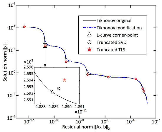
Figure 2.
Numerical difference of least square parameters using different regularization methods.
2.3. RCR Method
The remove-compute-restore technique divides the geoid undulation into three terms:
where long-wavelength term is the contribution of the Global Geopotential Model (GGM), is the indirect effect of the terrain on geoidal height, and is the residual geoidal height. The model geoid undulation can be obtained from the spherical harmonic coefficient [34]:
where is the long radius of the reference ellipsoid, , and are the geocentric latitude, longitude, and radial diameter of the calculated point, respectively; and are the fully normalized harmonic coefficients of the anomalous potential, is the fully normalized Legendre function.
Indirect terrain impact refers to changes in the geoid due to removal of the terrain effect. This effect can be calculated from elevation data, for example, by [35]:
where and are the heights of the computation and running points, respectively, is the plane distance between two points.
The residual geoid height represents the high frequency information of the geoid. The calculation formula is [3]:
where is the original Stokes’ function in Equation (2), and is computed by:
where and represent surface measured free-air gravity anomaly and GGM gravity anomalies, respectively, and is the terrain effect on gravity. The calculation formula can be expressed as [34]:
where max is the maximum complete order of GGM. In the case of using Helmert condensation to reduce the gravity anomalies [45], the terrain effect can be calculated as:
3. Results
3.1. Accuracy Comparison Between XGM2016 and EGM2008
This paper evaluated the applicability of EGM2008 and XGM2016 models in the study area using GPS-leveling points distributed in Jilin Province. The results are shown in Table 2. The standard deviation of XGM2016 was 1 cm higher than that of EGM2008 in Jilin Province, with an error range about 7 cm higher. The mean differences of the EGM2008 and XGM2016 geoid heights were up to 27.2 and 28.9 cm, respectively.
Table 2.
Comparison of EGM2008 and XGM2016 geoid heights with GPS/leveling derived ones in Jilin Province (cm).
For area A, the standard deviation and error range of EGM2008 were ± 5.8 and 27.1 cm, respectively, and the standard deviation and error range of XGM2016 in Areas A were ± 5.5 and 23.5 cm. XGM2016 was slightly more accurate than EGM2008 in plain Area A, with a lower error range. For area B, the standard deviation and error range of the original EGM2008 model were ± 5.9 and 25.3 cm, respectively. The standard deviation and error range of the original XGM2016 model in Areas B were ± 7.3 and 31.7 cm, respectively. The accuracy of XGM2016 was relatively lower due to its lower resolution. A detailed comparison is presented in the following sections.
The degree of geoid height calculated by the EGM2008 model was set to 719 to maintain the same complete degree/order in the two models. The results show that the maximum, minimum, mean, and standard deviation in the plain area were 1.6, - 29.9, - 13.6 and ± 6.3 cm, respectively, and 2.4, - 31.9, - 13.1, and 7.0 cm in the high mountainous areas, respectively. XGM2016 was more accurate in the plain area, whereas the accuracies of the two models were similar in the mountainous areas.
The gridded free-air gravity anomalies obtained from the terrestrial gravity data distributed within 0.5 ° of Areas A and B are shown in Figure 3. The differences between the gravity anomalies calculated by EGM2008 and XGM2016 models are shown in Table 3. Statistics of the gravity anomalies and the reduced ones were shown in Table 3 to illustrate the applicability of the RCR method in the study area.
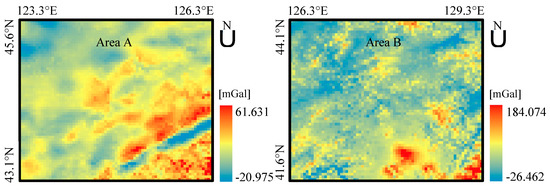
Figure 3.
The gridded free-air gravity anomalies in Area A and B.
Table 3.
Statistics of the gravity anomalies and the reduced ones (mGal).
3.1.1. Fixed Parameters
The gravity anomaly degree variances were calculated from the gravity field model coefficients, and the geopotential harmonic error degree variances were calculated from the gravity field model coefficient error, as shown in Figure 4. The gravity anomaly degree variances of XGM2016 and EGM2008 were consistent in up to degree 715, with an average value difference of 1.88% and an extreme value of no more than 7.86%. The gravity anomaly degree variances of XGM2016 decreased significantly after 715, and EGM2008 also decreased after 2160. The geopotential harmonic error degree variances of XGM2016 were significantly lower than those of EGM2008, and the value dropped significantly after degree 680.
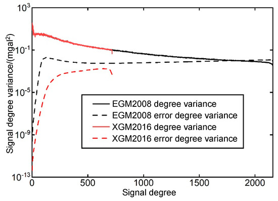
Figure 4.
Signal degree variance of EGM2008 and XGM2016.
The contribution of the low-degree coefficients of the model and their errors to the global mean square error became more prominent for the modification of the original Stokes kernel function by KTH although the complete degree of the XGM2016 and EGM2008 global gravity field models was different. The higher degree of EGM2008 model indicates a larger infinite truncation, which introduced more coefficient errors into the calculation of global mean square error, making the EGM2008 model less dominant in the KTH method. The higher precision of the longer-wavelength component in XGM2016 reduced the influence of the model coefficients and their errors to the global mean square error, such that a better geoid can be obtained, while other parameters (modification limits, integral radius and terrestrial gravity data error) were unchanged.
3.1.2. Optional Parameters
The selection of the upper limit of the truncation degree of the gravity field model should fully use the long-wavelength component of the gravity field model and reduce the errors caused by the excessive value of the model degree. The upper limit of the harmonic function was guaranteed to minimize the effect of the modified Stokes formula outside the integral radius [17]. The two upper limits are usually equal by default in the calculation of the least squares modified Stokes formula [17], and we applied the same default. Terrestrial gravity data error variance was set to 1 mgal2, the infinite truncation degrees of EGM2008 and XGM2016 were 2000 and 719, respectively, and the integral radii were 1°, 2° and 3° respectively. The difference between the and values based on EGM2008 and XGM2016 on the global mean square error is shown in Figure 5.
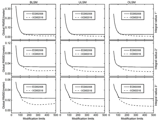
Figure 5.
The global Root Mean Squared Error (RMSE) obtained by different modification limits. The horizontal and vertical axes represent the modification limits [0, 500] and global RMSE, respectively. Each row corresponds to a fixed integral radius, and each column corresponds to a fixed stochastic model.
For the global mean square error with same integral radius, BLSM and OLSM produced the maximum and minimum values, respectively, and ULSM produced a similar error to OLSM with a numerical difference of less than10−5 m (EGM2008) or 10−6 (XGM2016). The difference between the three modification methods was slight when the modification limits were less than 100, but increased substantially when the modification limits increased to 200, and a stable difference was observed when the modification limits increased over 300. The global mean square errors of XGM2016 was 2 cm lower than that of EGM2008 when the modification limits were above 300. With increasing integral radius, the global mean square errors in both gravity models showed a decreasing tendency—from the decimeter to millimeter level when the modification limits increased. This occurred because the increase in integral radius absorbed more terrestrial gravity data into the calculation, and the contribution of short-wavelength component from terrestrial gravity data decreased with increasing long-wavelength component in the gravity field model. In general, the global mean square error of the XGM2016 model was lower than that of EGM2008 in the three least squares modification methods, and the mutual difference between the two models was less than 2 mm when the modification limits were greater than 300. In the subsequent analysis, the modification limits were set at 300.
The difference between the modified Stokes kernel function and the original Stokes kernel function in XGM2016 and EGM2008 is shown in Figure 6. The modified Stokes kernel function of XGM2016 decreased rapidly compared to that of EGM2008 in the three least squares modification methods. XGM2016 increased more rapidly after the two models reached their respective minimum values, which resulted in a better approximation of zero.
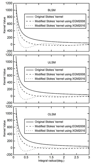
Figure 6.
Difference between original Stokes’ kernel and modified Stokes’ kernel. The horizontal and vertical axes represent the integral radius [0, 3] and value of Stokes kernel, respectively.
The integral radius was then set to , and the terrestrial gravity data error variance was set to 1, 4 and 9 mgal2.The global mean square error of EGM2008 and XGM2016 varied with the integral radius, as shown in Figure 7. The highest values for the global mean square error were obtained with the BLSM, while the lowest ones were with the OLSM. OLSM and ULSM have similar error values with a numerical difference less than 10−6 m (EGM2008) or 10−8 m (XGM2016). The numerical difference of the global mean square error between BLSM and ULSM / OLSM increases as the terrestrial gravity data error variance increases. The global mean square error calculated by OLSM decreased in the range of cm compared with the EGM2008 model as the variance of terrestrial gravity error increased.

Figure 7.
The global RMSE obtained by different integral radius. The horizontal and vertical axes represent the integral radius [0, 10] and global RMSE, respectively.
The terrestrial gravity error variance was set to 0 mgal2 to analyze the proportion of the coefficient error and the integral truncation error in the global mean square error. The global mean square errors of both models were at the millimeter level when the integral radius was increased to 2° (Figure 8.). The global mean square error calculated by the two models was basically above 1 cm when the terrestrial gravity data error was 1, 4 and 9 mgal2 and the integral radius was greater than 2° compared with Figure 7, which showed that the terrestrial gravity error occupied the major part of the global mean square error in the KTH-refined geoid.
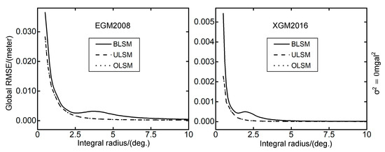
Figure 8.
The global RMSE obtained by different integral radius (). The horizontal and vertical axes represent the integral radius [0, 10] and global RMSE, respectively.
The terrestrial gravity data error variance and the model coefficient error variance were set to 0 mgal2 to determine the proportion of the truncation error term in the global mean square error (Figure 9). The global mean square error was in the millimeter level when the integral radius was less than 2°, and close to 0 when the integral radius was greater than 2°, indicating that the influence of the truncation error was extremely limited. The numerical difference was only about 10−5 when the integral radius was the same.
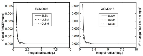
Figure 9.
The global RMSE obtained by different integral radius ( and ). The horizontal and vertical axes represent the integral radius [0, 10] and global RMSE, respectively.
3.1.3. External Parameters
The terrestrial gravity data were not error-free, and the KTH method requires determination of the terrestrial gravity data error variance. Prior to this section, we set the error as a constant. To highlight the contribution of different external parameters to the global mean square error, the cumulative sum of terrestrial gravity data errors in the global mean square error with the increase of infinite truncation (( in Equation (5)) is shown in Figure 10. The terrestrial gravity data error variance was set to 0, 1, 4, and 9 mgal2. For the terrestrial gravity data error, the impact on BLSM and OLSM was maximum and minimum, respectively, and ULSM showed a similar error to OLSM with a numerical difference less than 10−6 m (EGM2008) or 10−7 m (XGM2016). The global mean square error of the two models increased and gradually flattened as the infinite truncation increased. The global mean square error accumulation of XGM2016 in the three modification methods was less than that of EGM2008 when the infinity truncation was unchanged, which indicated that XGM2016 in the KTH method-refined geoid was less sensitive to terrestrial gravity data than EGM2008.
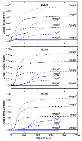
Figure 10.
Cumulative sum of terrestrial gravity data errors in the global RMSE (black line: EGM2008; blue line: XGM2016).
The above comparison of the EGM2008 and XGM2016 models is based on the influence of various parameters in the KTH method on the global mean square error (Equation (5)). The modification parameters, including the coefficients and errors of the global gravity field model ( and ), the modification limits (), the integration radius (), and the terrestrial gravity data error variance () can significantly affect the magnitude of the global mean square error. Decomposing Equation 5 into three parts, the terrestrial gravity data error variance and model coefficient error produce a significant part of the global mean square error, and the truncated error term is basically zero after the integration radius is greater than 2° The analysis results of the XGM2016 model are significantly more accurate than EGM2008 for each solution.
3.2. Comparison of Accuracy of Refinement Geoid
3.2.1. Plain Area
We analyzed the refined geoid in the plain area in Jilin Province (Area A) using RCR and KTH method based on EGM2008 and XGM2016. After repeated and careful trials, as well as consideration of the distribution of terrestrial gravity data, the calculated integral radius of the RCR residual geoid was limited to 0.5° and the indirect influence was set at 2°. To facilitate the distinction between subsequent results, the results of EGM2008 and XGM2016 are called RCR08-A and RCR16-A, respectively.
This paper used the Helmert condensation method with an RCR procedure for computation of the RCR08-A and RCR16-A models, and all constituents of the refined geoid in the plain area based on the RCR method of EGM2008 and XGM2016 are shown in Figure 11. The three constituents of the refined model, including the contribution of the GGMs, the indirect effect on geoid height, and the residual geoid height, are given in Equations (21), (22) and (23), respectively. The refined models and the model’s contribution displayed some similarities due to the smooth topography of Area A. The residual geoids of the two models show a decimeter difference, in accordance with Table 3. Since the indirect effect on geoid height is only related to height (Equation (22)), the calculation amount in Area A is the same (Figure 11c).
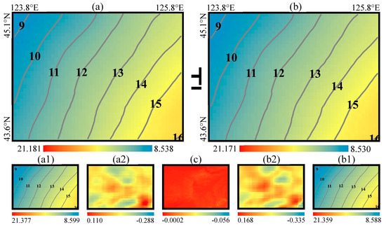
Figure 11.
RCR-refined geoid and its constituents in Area A. (a) Geoid heights of the RCR08-A: (a1) Contribution of the EGM2008 , (a2) Residual geoid height ; (b) Geoid heights of the RCR16-A: (b1) Contribution of the XGM2016 , (b2) Residual geoid height , (c) Indirect effect on geoid height . Unit: meter.
The results of the accuracy comparison are shown in Table 4. We used the least squares adjustment combined with the four-parameter model and seven-parameter fit [46] to model the residuals, systematic errors, and datum inconsistencies between the gravimetric geoid heights and the GPS-leveling ones.
Table 4.
Comparison of EGM2008 and XGM2016 RCR-geoid heights with GPS/leveling derived ones in Area A (cm).
The four-parameter model is given as:
and the seven-parameter model is:
where and are the geodetic latitude and longitude of the GPS-leveling point, respectively.
where is the first eccentricity of the reference ellipsoid. The matrix system of observation is:
then the estimated parameters are:
The results of fitting using the parametric model are shown in Table 4, and the fitting methods were applied to correct the systematic errors in the following sections. The standard deviation and error range of the refined RCR08-A model decreased to ± 3.1 and 13.9 cm, respectively, whereas the standard deviation and error range of the refined RCR16-A model decreased to ± 3.2 and 14.7 cm, respectively. The mean differences of RCR08-A and RCR16-A were 22.1 and 20.9 cm, respectively. After four-parameter fitting, the standard deviations of both models decreased by ± 0.2 cm. The seven-parameter fitting produced more accurate results, of which the accuracy of RCR08-A was optimal in Area A, and the standard deviation reached ± 2.5 cm.
Some of the values of modification parameters needed to be determined prior to calculation of the approximate geoid undulation using the KTH method. After tests to determine the unified modification parameters, the integral radius was set to 0.5°, the terrestrial gravity data error variance was set to 1 mgal2, and the modification limits were set as . To facilitate the distinction between subsequent results, the results of EGM2008 and XGM2016 are called KTH08-A and KTH16-A, respectively.
The refined geoids and all their corrections in the plain area based on the KTH method of EGM2008 and XGM2016 are shown in Figure 12. The combined atmospheric correction, including the sum of the direct and indirect atmospherical effects and the ellipsoidal correction given by Equations (10) and (16), respectively, had only a sub-millimeter-level correction in Area A. The combined topographic correction, including the sum of the direct and indirect topographical effects and the downward continuation effect, accounted for the major part of the correction. The approximate geoid undulation was highly similar to the refined model, whereas the latter narrows the range of high values of the geoid to smooth the results. Since the combined topographic correction is only related to the height (Equation (9)), the calculation amount in Area A is the same (Figure 12c).
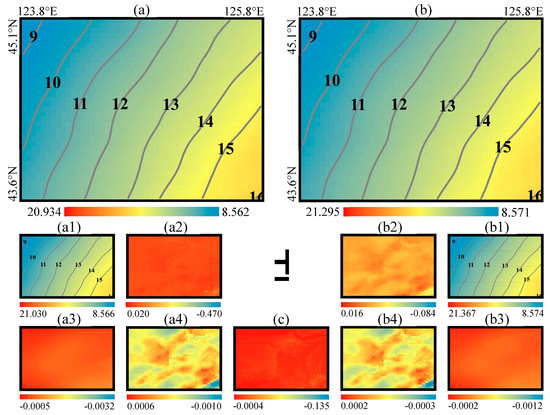
Figure 12.
KTH-refined geoid and its corrections in Area A. (a) Geoid heights of the KTH08-A, (a1) approximate geoid undulation , (a2) Downward continuation correction , (a3) Combined atmospheric correction , (a4) Ellipsoidal correction ; (b) Geoid heights of the KTH16-A, (b1) The approximate geoid undulation , (b2) Downward continuation correction , (b3) Combined atmospheric correction , (b4) Ellipsoidal correction ; (c) Combined topographic correction . Unit: meter.
The results of the accuracy comparison are shown in Table 5. The standard deviation and the error range of the refined KTH08-A model decreased to ± 3.6 and 14.0 cm, respectively, and to ± 2.8 and 13.3 cm for the refined KTH16-A model, respectively. After four-parameter fitting, the standard deviations of both models decreased by about ± 0.3 cm. We observed that the seven-parameter fitting also produced more accurate results and significantly reduced the standard deviation of the KTH08-A model to 2.0 cm. Compared with Table 4, we found that for Area A, XGM2016 is slightly more accurate than RCR overall based on the KTH method, whether before or after fitting. EGM2008 based on KTH was more accurate than the RCR method only after seven-parameter fitting. However, the differences between the solutions were only at the millimeter level under the same conditions.
Table 5.
Comparison of EGM2008 and XGM2016 KTH-geoid heights with GPS/leveling derived ones in Area A (cm).
3.2.2. Mountainous Area
The refined geoid in the mountainous area provided a more obvious comparison of the results with more complicated terrain and the sparse distribution of terrestrial gravity data. For determination of the aforementioned modification parameters, the terrestrial gravity data error variance for Area B was modified to be 9 mgal2 and other parameters were set equal to the values used for the plain area.
All constituents of the refined geoid in the mountainous area based on the RCR method of EGM2008 and XGM2016 are shown in Figure 13. Compared with Area A, the result of the refined geoid in Area B changed more drastically than the contribution of GGMs, and the indirect effect on geoid height also increased by an order of magnitude to the centimeter or even decimeter level. Judging from the difference in the reduction of gravity anomalies (Table 3), the residual geoids of the two models are noticeably different compared with the plain area.
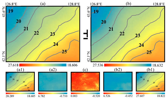
Figure 13.
RCR-refined geoid and its constituents in Area B. (a) Geoid heights of RCR08-B, (a1) Contribution of the EGM2008 , (a2) Residual geoid height ; (b) Geoid heights of the RCR16-B, (b1) Contribution of the XGM2016 , (b2) Residual geoid height ; (c) Indirect effect on geoid height . Unit: meter.
Table 6.
Comparison of EGM2008 and XGM2016 RCR-geoid heights with GPS/leveling derived ones in Area B (cm).
Table 7.
Comparison of EGM2008 and XGM2016 KTH-geoid heights with GPS/leveling derived ones in Area B (cm).
Compared with Table 2, the standard deviation and error range of the refined RCR08-B model decreased to ± 4.4 and 13.6 cm, respectively, and to ± 4.6 and 15.9 cm for the refined RCR16-B model, respectively. The mean differences for RCR08-B and RCR16-B were 21.1 and 21.9 cm, respectively. Similar to the previous section, the seven-parameter fitting demonstrated more accurate modeling. The STD decreased by more than ± 1 cm both in RCR08-B and RCR16-B, while the range has been reduced by 2.2 and 3.3 cm, respectively.
The refined geoids and all their corrections in the mountainous area based on the KTH method of EGM2008 and XGM2016 are shown in Figure 14. Similar to the situation in Area A, the magnitudes of the combined atmospheric correction and ellipsoid correction in the Area B are also very small. The combined topographic correction and the downward continuation effect accounted for majority of the correction. Compared with the approximate geoid undulation, the refined model not only highlighted the details of the local area, but also reduced the range of the regional geoid level.
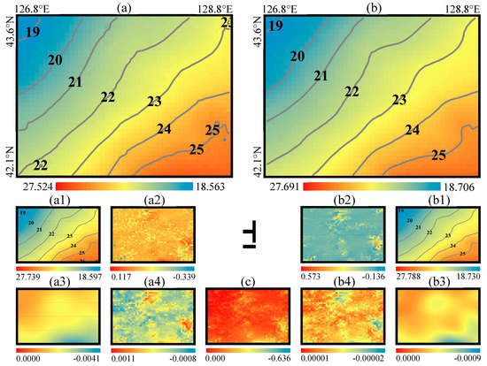
Figure 14.
KTH-refined geoid and its corrections in Area B. (a) Geoid heights of the KTH08-B, (a1) The approximate geoid undulation , (a2) Downward continuation correction , (a3) Combined atmospheric correction , (a4) Ellipsoidal correction ; (b) Geoid heights of the KTH16-B, (b1) The approximate geoid undulation , (b2) Downward continuation correction , (b3) Combined atmospheric correction , (b4) Ellipsoidal correction ; (c) Combined topographic correction . Unit: meter.
The standard deviation and error range of the refined KTH08-B model decreased to ± 4.0 and 14.8 cm, respectively, and to ± 4.1 and 13.4 cm for the refined KTH16-B model, respectively. Similarly, EGM2008 model based on the KTH method was the most accurate after seven-parameter fitting, and the standard deviation was reduced to 2.4 cm. Compared with Table 6, the overall results produced using the KTH method were slightly better than the RCR method. However, the differences between the solutions were still only at the millimeter level under the same conditions.
4. Conclusions
In this study, we evaluated the performance differences between EGM2008 and XGM2016 based on the effects of the modification parameters on the global mean square error in the KTH method. The value of the modification limits was determined by the influence of the modification limits on the global mean square error between EGM2008 and XGM2016. We analyzed the model coefficients and sensitivity to the terrestrial gravity data error. To identify the influence of the integral radius on the global square error, we produced a curve with higher resolution on the basis of a previous study [25] that delineates the global square error with more detailed fluctuation. The coefficient error of the XGM2016 model was lower than that of the EGM2008 model on the same degree, although we found little difference in the model coefficients between the two gravity field models. The terrestrial gravity data error was the main parameter affecting the accuracy of the KTH method. The influence of each parameter on the global mean square error showed that the precision of XGM2016 was significantly higher than that of EGM2008.
The RCR method refined the geoid by using 2D-FFT to increase calculation speed, and the indirect terrain impact was usually proportional to the terrain height with centimeter level in the plain area and decimeter level or even meter level in the mountain area, which significantly reduces the extreme value of the error and cannot be ignored in the refinement process. The modified Stokes kernel was not applied in the RCR method, making it insensitive to terrestrial gravity data error and coefficient errors. This insensitivity deteriorated in the mountainous areas with sparse terrestrial gravity data and higher undulation of indirect impact, and the refined geoid showed a lower accuracy than that of the KTH method.
The key of the KTH method is to determine the least square parameter , which is related to the calculation of the approximate geoid undulation . and are related to the calculation of the three corrections within the addictive corrections, except the combined topographic correction . The majority of the correction was due to the downward continuation effect and the combined topographic correction . The values of the ellipsoidal correction and the combined atmospheric correction were usually at the millimeter level in the study area. The refined geoid was smoothened after application of the additive corrections because these corrections decreased the distribution range of the regional geoid value in the study area, whereas the accuracy of the refined geoid decreased about 1 cm after the additional corrections, which indicates that the approximate geoid undulation is already highly accurate in the study area.
The solutions of the KTH method based on EGM2008 and XGM2016 models were slightly more accurate than those of the RCR method in the mountainous areas regardless of fitting being applied, which showed that the KTH method may be more suitable for mountainous areas where the terrestrial gravity data are sparse and unevenly distributed. The millimeter difference between the computed solutions was lower than the accuracy of the GPS-leveling in the study area, and we think that the KTH and RCR methods are equally applicable in this experimental area.
This study applied the four-parameter and seven-parameter models to reduce the systematic error between gravimetric geoid and GPS-leveling derived geoid heights. The seven-parameter model was the most accurate of the two, and standard deviation decreased by about 1 cm in high mountainous areas (Table 4, Table 5, Table 6 and Table 7).
The gravity field model used by the KTH method did not necessarily produce more accurate refinement results of increasing degree because the modification of the Stokes formula by the KTH method mainly used the long-wavelength component of the gravity field model, and the model with a low-degree coefficient error seemed more suitable. The short-wavelength component of the KTH method was mainly provided by the terrestrial gravity data, which may highly affect the resolution and accuracy of the refined geoid. The improvement in density and accuracy of the terrestrial gravity data may be an effective way to improve the KTH geoid refinement.
Author Contributions
Conceptualization, H.L. and H.W.; Data curation and validation, B.W.; Formal analysis, H.W.; Methodology, Q.W. and H.W.; Writing—original draft, Q.W., Funding acquisition, S.C. All authors have read and agreed to the published version of the manuscript.
Funding
This research was funded by the Program for JLU Science and Technology Innovative Research Team (JLUSTIRT, 2017TD-26).
Conflicts of Interest
The authors declare that they do not have any conflicts of interest.
References
- Molodenskii, M. Methods for Study of the External Gravitational Field and Figure of the Earth; Jerusalem, Israel Program for Scientific Translations, 1962; The Office of Technical Services, United States Department of Commerce: Washington, DC, USA, 1962. [Google Scholar]
- Schwarz, K.; Sideris, M.; Forsberg, R. The Use of FFT Techniques in Physical Geodesy. Geophys. J. Int. 1990, 100, 485–514. [Google Scholar] [CrossRef]
- Sjöberg, L.E. A discussion on the approximations made in the practical implementation of the remove–compute–restore technique in regional geoid modelling. J. Geod. 2005, 78, 645–653. [Google Scholar] [CrossRef]
- Ayhan, M.E. Geoid determination in Turkey (TG-91). Bull. Géodésique 1993, 67, 10. [Google Scholar] [CrossRef]
- Fotopoulos, G.; Kotsakis, C.; Sideris, M. A new Canadian geoid model in support of levelling by GPS. Geomatica 2000, 54, 53–62. [Google Scholar] [CrossRef]
- Zhang, K.; Featherstone, W.; Stewart, M.; Dodson, A. A new gravimetric geoid of Australia. In Proceedings of the Second Continental Workshop on the Geoid in Europe, Budapest, Hungary, 10–14 March 1998; Volume 4, pp. 225–234. [Google Scholar]
- Smith, D.A.; Milbert, D.G. The GEOID96 high-resolution geoid height model for the United States. J. Geod. 1999, 73, 219–236. [Google Scholar] [CrossRef]
- Odera, P.A.; Fukuda, Y.; Kuroishi, Y. A high-resolution gravimetric geoid model for Japan from EGM2008 and local gravity data. Earth Planets Space 2012, 64, 361–368. [Google Scholar] [CrossRef]
- Sjöberg, L.E. Least squares combination of satellite harmonics and integral formulas in physical geodesy. Gerlands Beitraege Geophys. 1980, 89, 371–377. [Google Scholar]
- Sjöberg, L.E. Least squares combination of satellite and terrestrial data in physical geodesy. Ann. Geophys. 1981, 37, 25–30. [Google Scholar]
- Neyman, Y.M.; Li, J.; Liu, Q. Modification of Stokes and Vening-Meinesz formulas for the inner zone of arbitrary shape by minimization of upper bound truncation errors. J. Geod. 1996, 70, 410–418. [Google Scholar] [CrossRef]
- Ellmann, A. On the Numerical Solution of Parameters of the Least Squares Modification of Stokes’ Formula. In A Window on the Future of Geodesy; Berlin, S.F., Ed.; Springer: Heidelberg/Berlin, Germany, 2005; pp. 403–408. [Google Scholar] [CrossRef]
- Sjöberg, L.E. Least Squares Modification of Stokes’ and Vening Meinesz’formulas by Accounting for Errors of Truncation, Potential Coefficients and Gravity Data; University of Uppsala, Institute of Geophysics, Department of Geodesy: Uppsala, Sweden, 1984. [Google Scholar]
- Sjöberg, L.E. Refined least squares modification of Stokes’ formula. Manuscr. Geod. 1991, 16, 367–375. [Google Scholar]
- Sjöberg, L.E. A general model for modifying Stokes’ formula and its least-squares solution. J. Geod. 2003, 77, 459–464. [Google Scholar] [CrossRef]
- Ågren, J.; Sjöberg, L.E.; Kiamehr, R. The new gravimetric quasigeoid model KTH08 over Sweden. J. Appl. Geod. 2009, 3, 143–153. [Google Scholar] [CrossRef]
- Ellmann, A. The Geoid for the Baltic Countries Determined by the Least Squares Modification of Stokes’ Formula. Ph.D. Thesis, Royal Institute of Technology (KTH), Department of Infrastructure, Stockholm, Sweden, 2004. [Google Scholar]
- Ellmann, A. Two deterministic and three stochastic modifications of Stokes’s formula: A case study for the Baltic countries. J. Geod. 2005, 79, 11–23. [Google Scholar] [CrossRef]
- Kiamehr, R. Precise Gravimetric Geoid Model for Iran Based on GRACE and SRTM Data and the Least-Squares Modification of Stokes’ Formula: With Some Geodynamic Interpretations. Ph.D. Thesis, Royal Institute of Technology (KTH), Department of Infrastructure, Stockholm, Sweden, 2006. [Google Scholar]
- Ulotu, P. Geoid Model of Tanzania from Sparse and Varying Gravity Data Density by the KTH Method. Ph.D. Thesis, Royal Institute of Technology (KTH), Department of Infrastructure, Stockholm, Sweden, 2009. [Google Scholar]
- Abdalla, A.; Fairhead, D. A new gravimetric geoid model for Sudan using the KTH method. J. Afr. Earth Sci. 2011, 60, 213–221. [Google Scholar] [CrossRef]
- Abbak, R.A.; Erol, B.; Ustun, A. Comparison of the KTH and remove–compute–restore techniques to geoid modelling in a mountainous area. Comput. Geosci. 2012, 48, 31–40. [Google Scholar] [CrossRef]
- Sjöberg, L.; Gidudu, A.; Ssengendo, R. The Uganda gravimetric geoid model 2014 computed by the KTH method. J. Geod. Sci. 2015, 5. [Google Scholar] [CrossRef]
- Pavlis, N.K.; Holmes, S.A.; Kenyon, S.C.; Factor, J.K. The EGM2008 Global Gravitational Model. In AGU Fall Meeting Abstracts; American Geophysical Union: Washington, DC, USA, 2008. [Google Scholar] [CrossRef]
- Eshagh, M. Least-squares modification of stokes’ formula with EGM08. Geod. Cartogr. 2009, 35. [Google Scholar] [CrossRef]
- Eshagh, M. A strategy towards an EGM08-based Fennoscandian geoid model. J. Appl. Geophys. 2012, 87, 53–59. [Google Scholar] [CrossRef]
- Barnes, D.; Holmes, S.; Factor, J.; Ingalls, S.; Presicci, M.; Beale, J. Earth Gravitational Model 2020. In Proceedings of the EGU General Assembly Conference Abstracts, Thessaloniki, Greece, 19–23 September 2017. [Google Scholar]
- Pail, R.; Fecher, T.; Barnes, D.; Factor, J.F.; Holmes, S.A.; Gruber, T.; Zingerle, P. Short note: The experimental geopotential model XGM2016. J. Geod. 2018, 92, 443–451. [Google Scholar] [CrossRef]
- Ågren, J.; Sjöberg, L.E. Comparison of some Methods for Modifying Stokes’ Formula in the GOCE Era. In Proceedings of the Second International GOCE User Workshop “GOCE, the Geoid and Oceanography”, ESA-ESRIN, Frascati, Italy, 8–10 March 2004. [Google Scholar]
- Yildiz, H.; Forsberg, R.; Ågren, J.; Tscherning, C.; Sjöberg, L.E. Comparison of remove-compute-restore and least squares modification of Stokes’ formula techniques to quasi-geoid determination over the Auvergne test area. J. Geod. Sci. 2012, 2, 53–64. [Google Scholar] [CrossRef]
- Abdalla, A.; Green, C. Utilisation of Fast Fourier Transform and Least-squares Modification of Stokes formula to compile a gravimetric geoid model over Khartoum State: Sudan. Arab. J. Geosci. 2016, 9, 236. [Google Scholar] [CrossRef]
- Hennig, T.; Kretsch, J.; Pessagno, C.; Salamonowicz, P.; Stein, W. The Shuttle Radar Topography Mission. In Digital Earth Moving; Westort, C.Y., Ed.; Springer: Berlin/Heidelberg, Germany, 2001; pp. 65–77. [Google Scholar] [CrossRef]
- Becker, J.; Sandwell, D.; Smith, W.; Braud, J.; Binder, B.; Depner, J.; Fabre, D.; Factor, J.; Ingalls, S.; Kim, S.H.; et al. Global bathymetry and elevation data at 30 arc seconds resolution: SRTM30_PLUS. Mar. Geod. 2009, 32, 355–371. [Google Scholar] [CrossRef]
- Heiskanen, W.A.; Moritz, H. Physical geodesy. Bull. Géodésique (1946–1975) 1967, 86, 491–492. [Google Scholar] [CrossRef]
- Sideris, M.; She, B. A new, high-resolution geoid for Canada and part of the U.S. by the 1D-FFT method. Bull. Géodésique 1995, 69, 92–108. [Google Scholar] [CrossRef]
- Ellmann, A. Computation of three stochastic modifications of Stokes’s formula for regional geoid determination. Comput. Geosci. 2005, 31, 742–755. [Google Scholar] [CrossRef]
- Paul, M.K. A method of evaluating the truncation error coefficients for geoidal height. Bull. Géodésique 1973, 110, 413–425. [Google Scholar] [CrossRef]
- Sjöberg, L.E. The topographic bias by analytical continuation in physical geodesy. J. Geod. 2007, 81, 345–350. [Google Scholar] [CrossRef]
- Sjöberg, L.E. Topographic and atmospheric corrections of gravimetric geoid determination with special emphasis on the effects of harmonics of degrees zero and one. J. Geod. 2001, 75, 283–290. [Google Scholar] [CrossRef]
- Sjöberg, L.E.; Nahavandchi, H. The atmospheric geoid effects in Stokes’ formula. Geophys. J. Int. 2000, 140, 95–100. [Google Scholar] [CrossRef]
- Sjöberg, L.E. A solution to the downward continuation effect on the geoid determined by Stokes’ formula. J. Geod. 2003, 77, 94–100. [Google Scholar] [CrossRef]
- Ellmann, A.; Sjöberg, L. Ellipsoidal correction for the modified Stokes formula. Boll. Geod. Sci. Affin. 2004, 63, 153–172. [Google Scholar]
- Hansen, P.C. The discrete picard condition for discrete ill-posed problems. BIT Numer. Math. 1990, 30, 658–672. [Google Scholar] [CrossRef]
- Hansen, P.C. Rank-Deficient and Discrete Ill-Posed Problems (Numerical Aspects of Linear Inversion); SIAM: Philadelphia, PA, USA, 1998. [Google Scholar] [CrossRef]
- Omang, O.C.D.; Forsberg, R. How to handle topography in practical geoid determination: Three examples. J. Geod. 2000, 74, 458–466. [Google Scholar] [CrossRef]
- Kotsakis, C.; Sideris, M.G. On the adjustment of combined GPS/levelling/geoid networks. J. Geod. 1999, 73, 412–421. [Google Scholar] [CrossRef]


© 2020 by the authors. Licensee MDPI, Basel, Switzerland. This article is an open access article distributed under the terms and conditions of the Creative Commons Attribution (CC BY) license (http://creativecommons.org/licenses/by/4.0/).