Article

Correcting Image Refraction: Towards Accurate Aerial Image-Based Bathymetry Mapping in Shallow Waters

1
Lab of Photogrammetric Vision, Civil Engineering and Geomatics Dept., Cyprus University of Technology, 2-8 Saripolou str., 3036 Limassol, Cyprus
2
Department of Topography, School of Rural and Surveying Engineering, National Technical University of Athens, Zografou Campus, 9 Heroon Polytechniou str., 15780 Athens, Greece
*
Author to whom correspondence should be addressed.
Remote Sens. 2020, 12(2), 322; https://doi.org/10.3390/rs12020322
Submission received: 19 November 2019 / Revised: 4 January 2020 / Accepted: 14 January 2020 / Published: 18 January 2020

Abstract

:
Although aerial image-based bathymetric mapping can provide, unlike acoustic or LiDAR (Light Detection and Ranging) sensors, both water depth and visual information, water refraction poses significant challenges for accurate depth estimation. In order to tackle this challenge, we propose an image correction methodology, which first exploits recent machine learning procedures that recover depth from image-based dense point clouds and then corrects refraction on the original imaging dataset. This way, the structure from motion (SfM) and multi-view stereo (MVS) processing pipelines are executed on a refraction-free set of aerial datasets, resulting in highly accurate bathymetric maps. Performed experiments and validation were based on datasets acquired during optimal sea state conditions and derived from four different test-sites characterized by excellent sea bottom visibility and textured seabed. Results demonstrated the high potential of our approach, both in terms of bathymetric accuracy, as well as texture and orthoimage quality.

Graphical Abstract

1. Introduction

Compared with onshore aerial mapping, bathymetry mapping from aerial platforms in shallow waters is considered a much more time-consuming and costly process. However, it is still a more efficient operation than ship-borne echo-sounding methods or underwater photogrammetric methods [1], especially when it comes to shallower (less than 10 m depth) clearwater areas. A very important additional feature of image-based seabed mapping is that a permanent record of other features is obtained in the coastal region, such as tidal levels, coastal dunes, benthic communities, marine litter, rock platforms, and beach erosion [2]. These benefits are especially evident in the coastal zones of up to 10 m depth, in which most of the economic activities are concentrated, even though many alternatives for bathymetry have been reported recently [3]. Hence, this dynamically changing zone is prone to accretion or erosion and is an area in need of further methodological development, since there are no robust and cost-effective solutions for seamless underwater and overwater mapping tasks. On the one hand, image-based mapping techniques generally fail due to wave breaking effects and water refraction. On the other hand, echo-sounding techniques fail due to the short sensor-to-object distances [4]. At the same time, bathymetric LiDAR systems with concurrent imaging data acquisition deliver valuable and very accurate information, albeit at great cost, especially for small scale surveys. In addition, even though in terrestrial environments, multi-view stereo reconstruction and texture mapping pipelines can be executed operationally, this is not the same for the marine environment and, especially, for the seabed. In particular, despite the accurate and precise depth maps that can be derived from bathymetric LiDAR [5], the production of seabed orthoimages is still a challenging task due to refraction.
Towards this end, in this paper, we proposed an image-based refraction correction methodology based on the exploitation of structure from motion (SfM) and recent machine learning tools. The proposed approach corrects refraction in the image space and recovers in a reliable manner shallow bathymetric information from aerial imaging datasets acquired over calm water surfaces. The developed procedure can be integrated in a straight-forward way into modern photogrammetric workflows, based on SfM and multi-view stereo (MVS), supporting coastal engineering and mapping applications.

1.1. Related work and Contribution
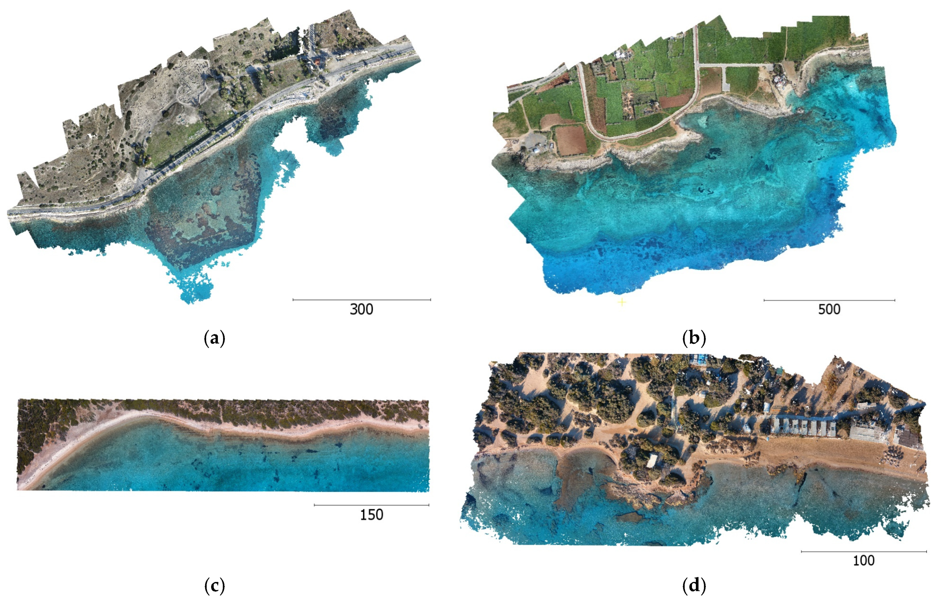
The adverse refraction effect has driven scholars to suggest several correction models for two-media photogrammetry, most of which are dedicated to specific applications generalized over many applications. The majority of these models are most commonly used in aerial photogrammetry for mapping large areas, while only a few of them were developed for close-range applications [6,7]. Two-media photogrammetric techniques first were reported in the early 1960s [8,9] and described the basic optical principles, proving that photogrammetric processing through water is possible. In the literature, two main approaches to correct refraction in through-water photogrammetry can be found: analytical or image-based. The first approach is based on the modification of the collinearity equation [7,10,11,12,13,14,15,16,17,18,19,20,21,22], while the latter is based on resampling the original image to correct for water refraction [4,6,23]. According to [10], there are two ways to analytically correct the effects of refraction in two-media photogrammetry: deterministic (explicit) or unsettled (ambiguous, iterative). The iterative method is employed to resolve the refraction effect, either in the object space [12] or in image space [10]. In the latter case, the whole multimedia problem is simplified to the radial shift computation module [23], which is the main concept of this study.
Authors in [6] corrected the refraction effect on the image by reprοcessing the radial distance of each pixel, according to a depth map derived for each image, of which the grey values were assigned according to the real depth, which was measured using traditional surveying techniques. Then, a new image was gradually constructed using the determined radial distances. The most recent approach to resolving the refraction effect in the image space is presented in [4]. These authors proposed an iterative simplified algorithm for water refraction correction within the existing photogrammetric pipeline. In this proposed correction model, a provisional DSM (digital surface model) was used in order to correct the refraction on the image iteratively. After computing a provisional but erroneous DSM, images were corrected from the refraction effect, and a new DSM was calculated using the corrected imagery. The solution converged after three to four iterations. Results over two test sites suggested that the mean distance between the LiDAR ground truth data and the resulting dense point clouds was between 0.20 m and 0.50 m, depending on the depth.
Finally, a new approach to correct the refraction on the image-based point clouds was suggested in [24,25], which also presented extensive research on the state of the art. In order to overcome the water refraction errors in a generic and accurate way, the authors employed machine learning tools, which can learn the systematic underestimation of the estimated depths. A support vector regression (SVR) model was developed, based on known depth observations from bathymetric LiDAR surveys, which was able to accurately recover bathymetry from point clouds derived from SfM-MVS procedures.
In the work reported here, a refraction correction methodology applied in image space is proposed, exploiting SfM and machine learning techniques. Instead of using the erroneous provisional DSMs and iterate the whole process three to four times (as suggested in [4]), which is a time-consuming and computationally expensive solution, a DSM created by the predicted corrected depths is used to correct the aerial imagery and facilitate orthoimages and textures generation. The correct DSM, which is fed into the algorithm is predicted using the SVR approach, originally presented in [24,25].
For a variety of applications, having the correct depth information solely in the form of point clouds, as resulting from the approach presented in [24,25], is not enough. Consequently, in the work presented here, the original imagery is also resampled to eliminate the refraction phenomenon. This facilitates a much more accurate and reliable SfM process, delivering a more accurate and reliable external and internal orientation of the images, directly related to the corrected DSM. This enables the faster and more accurate generation of orthoimagery and detailed textures of the 3D models of the seabed, which are very important for a number of applications, such as archeological or benthic community mapping and image-based seabed classification. Contrary to analytical correction approaches, the results of the proposed approach can be used by any SfM-MVS software in order to produce accurate bathymetric and visual results, while analytical correction approaches must be incorporated in the SfM-MVS process, which is not allowed in most commercial software. Compared with existing image-based approaches, the solution presented here proved to be more accurate and much faster than previously published works.
As with any method for seabed mapping using low-altitude aerial RGB imagery, the implementation of the proposed method is restricted by various environmental factors, including the sea state conditions, the visibility of the bottom, and the presence of texture on the seabed. To achieve accurate bathymetric results, the sea surface must be as flat as possible at the time of image acquisition in order to have optimal sea bottom visibility and satisfy the geometric assumption of a flat-water surface. In the case of a wavy surface, errors would be introduced [4,6,24,25,26,27]. Obviously, water turbidity and water visibility are additional constraints. The sea bottom must include texture, random patterns, and adequate features to ensure salient point detection and matching. Moreover, sun glint, which depends on the sun angle, may cause direct reflections on the water surface and create bright spots on images. Therefore, the sun elevation should be low during image acquisition (less than 30 degrees), with large angles of incidence with respect to the water surface and the sensor. Finally, caustics [1] may also appear in the aerial imagery, especially when the seabed of the shallower areas (less than 3 m depth) is imaged having a sun angle more than 30 degrees over the horizon, and small waves also exist. However, this phenomenon is eliminated when the ground sampling distance (GSD) is equal to or greater than the width of the caustics on the seabed, and no further actions should be taken in these cases.
The rest of the article is organized as follows: In Section 2, the datasets used are described, while, in Section 3, the proposed methodology is presented and justified. In Section 4, the tests performed and the experimental results are presented. Section 5 discusses the results of the proposed method, while Section 6 concludes the paper.

2. Datasets

The proposed methodology was applied in four different test areas in Cyprus and Greece with datasets acquired for real-world shallow bathymetry mapping tasks but under optimal sea state and water visibility conditions.

2.1. Agia Napa Test Area

The first area used is in Agia Napa, Cyprus, where the seabed reaches a depth of 14.8 m. The flight was executed with a Swinglet CAM fixed-wing UAV (unmanned aerial vehicle) with a Canon IXUS 220HS camera having 4.3 mm focal length, 1.55 μm pixel size, and 4000 × 3000 pixels. In total, 383 images were acquired, from an average flying height of approximately 209 m, resulting in a 6.3 cm average GSD (ground sampling distance). A total of 40 control points measured with RTK (real-time kinematic) accuracy (±0.03 m) were used, located only on land. The georeferencing achieved an RMSE (root mean square error) of 5.03, 4.74, 7.36 cm in X, Y, and Z, respectively, and average reprojection error of 1.11 pixels after the adjustment.

2.2. Amathounta Test Area

The second test area used is in Amathounta, Cyprus, where the seabed reaches a maximum depth of 5.57 m. The flight here was executed with the same UAV. A total of 182 images were acquired, from an average flying height of 103 m, resulting in 3.3 cm average GSD. A total of 29 control points measured with RTK accuracy were used, located only on land, resulting in an adjustment with RMSEs of 2.77, 3.33, 4.57 cm in X, Y, and Z, respectively, and a reprojection error of 0.645 pixels.

2.3. Cyclades-1 Test Area

The third area used is in Cyclades, Greece, where the seabed reaches a depth of 6.9 m. The flight was executed with a Phantom 4 UAV with an FC330 camera having a 3.61 mm focal length, 1.56 μm pixel size, and 4000 × 3000 pixels. In total, 449 images were acquired from three different average flying heights of approximately 88 m, 70 m, and 35 m. A total of 14 control points measured with RTK accuracy were used, located only on land. The georeferencing was realized with RMSE of 1.45, 1.03, 1.88 cm in X, Y, and Z, respectively, and an average reprojection error of 0.28 pixels after the adjustment.

2.4. Cyclades-2 Test Area

The fourth area used is also in Cyclades, Greece, where the seabed reaches a depth of 4.05 m. The flight was executed with the same Phantom 4 UAV with an FC330. In total, 203 images were acquired from two different average flying heights of approximately 75 m and 33 m. A total of 11 control points measured with RTK accuracy were used, located only on land. The georeferencing was realized with an RMSE of 2.03, 1.44, 2.13 cm in X, Y, and Z, respectively, and an average reprojection error of 0.30 pixels after the adjustment.
Table 1 presents the flights and image-based processing details of the four different test areas. It could be noticed that the four areas have different average flying heights, indicating that the suggested solution is not limited to specific flying heights or GSD’s. The common system used for measuring the ground control points (GCPs) for the test sites located in Cyprus was the Cyprus Geodetic Reference System (CGRS) 1993, while for the test sites located in Greece, the Greek Geodetic Reference System (GGRS) 1987 was used.

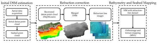
3. Proposed Methodology

As already mentioned, the straightforward way to apply water refraction correction into the existing pipeline of commercial SfM-MVS software is image transformation and resampling. However, in order to apply refraction correction, the focal distance, which varies per pixel depending on the air-water ratio [23], should be known a priori, which is not the case for any aerial data acquisition system.
In order to correct image refraction for aerial image-based bathymetry mapping, we propose a methodology that exploits recent machine learning tools able to estimate bathymetry in shallow waters. The overall architecture of the proposed approach is illustrated in Figure 1. Following aerial image data collection and Ground Control Points (GCPs) measurement, an initial SfM-MVS is executed. The resulting initial dense point cloud with systematic depth underestimation is corrected by employing the recently developed DepthLearn solution [24,25] for the seabed points. The updated (merged) DSM with recovered seabed bathymetry is used to differentially rectify the initial aerial image dataset. A new SfM is finally executed based on the refraction-free imaging dataset in order to update the interior and exterior orientation of the cameras, before orthomosaicing. During the last stages, texture and orthoimages can be generated based on the merged DSM generated by the corrected dense point clouds using DepthLearn [24,25] and the initial dry-land points. Details for every processing step are elaborated in the following subsections.

3.1. Initial DSM Estimation

3.1.1. Initial Dense Point Cloud

Following the aerial data acquisition step, a standard SfM-MVS approach should be employed in order to obtain the required data for applying the proposed refraction correction methodology (i.e., the interior and exterior orientation of the cameras and the initial dense point cloud (Figure 2)). Regarding the interior orientation of the cameras, a self-calibration approach was followed, and thus accurate GCPs’ measurements were of very high importance. In test areas like those used in this article, where GCPs were placed only on land, it is crucial to extend the GCPs’ covered area far from the shoreline, towards the land, in order to ensure a proper self-calibration, having GCPs scattered all over the images and to avoid large depth errors in the farthest parts of the block. In general, a minimum number of 10–15 GCPs are required for a reliable self-calibration [28].
For the SfM-MVS step, a specific software implementation does not affect the quality of the results, and they could be produced in a similar way using any commercial or open-source automated photogrammetric software, without employing any water refraction compensation. For the approach presented here, the Agisoft Metashape commercial software was used.

3.1.2. Seabed Point Cloud Extraction

The DepthLearn [24,25] correction tool should be applied only to the derived seabed points. Therefore, these points were extracted from the initial cloud. To perform this extraction, the points having an elevation equal or less than the sea surface level (measured at the time of the flight with an RTK Global Navigation Satellite System (GNSS) receiver) were considered as seabed points, while the rest as dry land points. A filtering step was then applied based on a Statistical Outlier Removal (SOR) [29] approach in order to remove noise from the point cloud and facilitate the creation of a more accurate DSM in the later steps. In particular, SOR is based on the distribution of point to k-nearest neighbor distances (in this paper, k = 8). For each point, the mean distance from it to all its neighbors is computed. By assuming that the resulting distribution is Gaussian with a local mean and a standard deviation, all points whose mean distances are outside an interval defined by the global distances mean and standard deviation can be considered as outliers and trimmed from the point cloud. This approach was considered necessary because image-based seabed point clouds produced using uncorrected imagery are prone to noise due to the effect of refraction on the Dense Image Matching (DIM) process, especially in deeper areas or areas with seagrass or poor texture [25]. In Figure 3, the seabed point clouds with natural colors (Figure 3a,b,e,f) are presented, while their corresponding bathymetry is illustrated in Figure 3c,d,g,h.

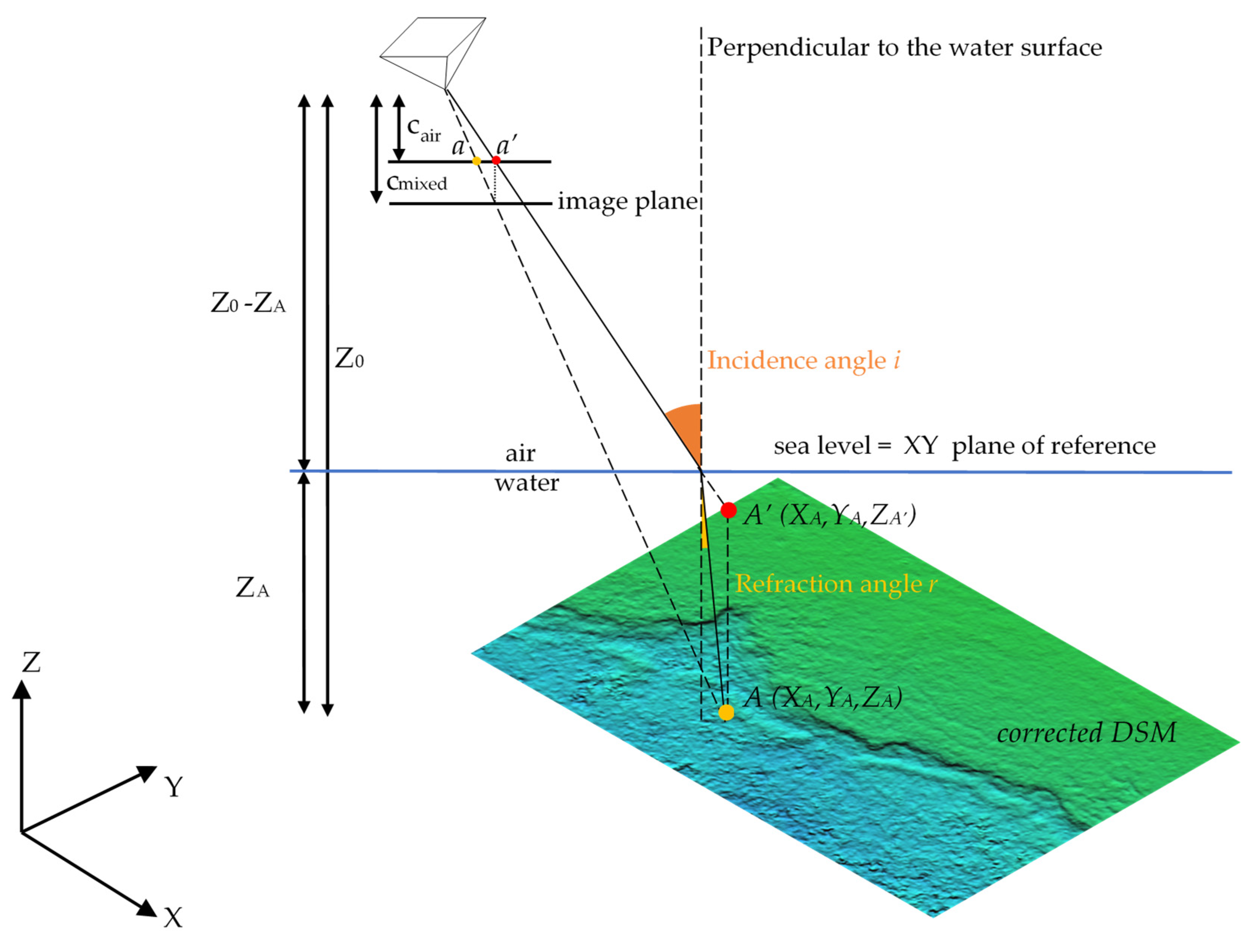
3.2. Refraction Correction

3.2.1. SVR-Based Refraction Correction on the Dense Point Clouds

The Support Vector Regression (SVR) method described in [24,25] was adopted in order to correct the apparent depth of each point of the initial seabed dense point clouds for the four test sites and produce the recovered dense point clouds. A linear SVR model describing the relation of the real (Z) and the apparent (Z0) with high accuracy was used to predict the correct depth of the erroneous point clouds. In [24,25], the SVR model fits according to the given training data; the LiDAR depths (Z) and the apparent depths (Z0) of a great number of 3D points. After fitting, the real depth can be predicted in the cases where only the apparent depth is available.
As concluded there, the developed SVR models have significant potential for generalization over different areas, and they can be used when no LiDAR data are available. As such, for the approach presented here, the already developed in [24,25] SVR model trained on Dekelia, i.e., on another test site, was used to predict the correct depths of the dense point clouds for the four test areas. The model of the Dekelia test site was selected since it is totally independent compared to the four test sites used in this article, thus proving, as well, the high potential of generalization capabilities of the models developed in [24,25]. It is important also to stress that the data used for training the Dekelia model were obtained with a different camera than the one used in Cyclades-1 and Cyclades-2 test sites and various flight patterns. This process went beyond currently available iterative approaches for image refraction correction because the bathymetric information is available a priori, facilitating faster and more accurate image correction.

3.2.2. Merged DSM Generation Using the Corrected Dense Point Clouds

After correcting the dense point clouds for refraction effects, a new DSM of the area was created. To achieve that, the recovered dense point clouds were first merged with the dry land dense points. This merged DSM was created directly in the geographic reference system where the camera positions were already calculated in order to facilitate later the calculation of ground intersections (X, Y, Z) using the projection center of the camera and the image coordinates of points. In Figure 4, the merged point clouds are illustrated with the same color-scale, while, in Figure 5, the generated merged DSMs of the four test areas are presented.
By visually comparing the seabed areas between Figure 4 and Figure 3c,d,g,h, the difference between the initial and the recovered depths could be observed. To highlight these differences, the depth of a point for each test site was reported in the initial (ZX in Figure 3) and the merged DSMs (ZX’ in Figure 4). These differences confirmed that the refraction effect cannot be ignored. Regarding merged DSM generation, for the Amathounta test site (Figure 5a), a ground sampling distance (GSD) of 0.13 m was achieved, for the Agia Napa test site (Figure 5b), a GSD of 0.28 m, for Cyclades-1 (Figure 5d), a GSD of 0.12 m, and for Cyclades-2 (Figure 5e), a GSD of 0.07 m, equal to the mean distance between the points of the dense point clouds of the four test sites, respectively.

3.2.3. Refraction Correction in the Image Space

In order to implement the refraction correction procedure, we followed certain principles. The relation between an object point on the seabed, camera position, and the respective image point is shown in Figure 6, where the air-water interface is assumed to be planar. The XY plane of the photogrammetric coordinate system X, Y, Z is defined as the boundary plane, hence Z = 0 for the sea level; the Z-axis is perpendicular to this plane with its positive direction upwards. Without the presence of the water, a seabed point A (XA, YA, ZA) is imaged at position a in the image plane, fulfilling the collinearity equation. However, when water is present, the seabed point A (XA, YA, ZA) is imaged at position a’ in the image plane due to the refraction effect. The apparent position of point A (XA, YA, ZA) is point A (XA, YA, ZA’), laying always in a shallower depth than the real point A (XA, YA, ZA), and the image point a is always closer to the projection of the principal point of the camera on the image plane than point a’. Considering this, the main aim of the image refraction correction approach presented here is to resample the original image containing image points like a’ to a refraction-free image containing image points like a   ( x α , y α ) .
Starting from a pixel a on the image plane having image coordinates (x, y), it is possible to estimate its seabed coordinates (XA, YA, ZA) using the interior and exterior orientation of the image, calculated already by the SfM process and the refraction corrected DSM (merged DSM). The line-surface intersection using a single collinearity function is an iterative process itself, but the Z component can be easily calculated. Also, exploiting the results of the SfM process, such as the georeferenced images following bundle adjustment, it is easy to identify if a point lies on the ground or the seabed by its height in the merged DSM. If point A has ZA above zero (usually zero is assigned to mean sea level), it can be omitted from further processing. If zero doesn’t correspond to sea level, then a reference point on the seashore, gathered during GCPs acquisition, may indicate the elevation of the water surface. That way, lakes could also be accommodated by a reference point in the shore and setting the water level Z in the code.
In particular, the refraction correction steps, implemented in MATLAB environment, were:
(a) Grid Creation
A grid was created based on the original image size and every 5 pixels. Then, it was duplicated into the transformed grid. The nodes of this grid would serve later as control points in the final image warping. Experiments performed also using a grid step of 1 pixel suggested that a grid step of 5 pixels was the fastest solution that did not compromise the accuracy of the results. This was because 5 pixels on the ground was almost equal to the GSD size of the merged DSM used for each of the test sites. As such, the area of 3 × 3 pixels in the interior of the 5 × 5 cell was smaller or equal to but not bigger than the GSD of the merged DSM. As a result, for each of the 3 × 3 pixels, in most cases, the same depth value was assigned.
(b) Interior Orientation
For every ( x α , y α ) point of the grid, the parameters of the interior orientation were applied, and the new position of the node ( x α , y α )’ was calculated. For the radial distortion, Brown’s model [30,31], formulated in Equation (1), was applied:
r a = r a ( 1 + k 1 r a 2 + k 2 r a 4 + k 3 r a 6 )
where k1, k2, k3 are the radial distortion coefficients, and r is the distance from a point ( x α , y α ) to the center of radial distortion.
For the tangential distortion, Equation (2), as formulated in [32], was used:
Δ x = [ P 1 ( r a 2 + 2 x α 2 ) + 2 P 2 x α y α ] [ 1 + P 3 r a 2 + P 4 r a 4 ] Δ y = [ 2 P 1 x α y α + P 2 ( r a 2 + 2 y α 2 ] [ 1 + P 3 r a 2 + P 4 r a 4 ]
where P1, P2, P3, and P4 are the tangential distortion coefficients of the lens, and r is the distance from a point ( x α , y α ) to the center of tangential distortion.
(c) Collinearity Equation Intersection with the Merged DSM
Then, the collinearity equation was applied, and its intersection (XA, YA, ZA) with the ground determined the point imaged at ( x α , y α )’, as calculated using the available georeferenced DSM.
(d) cmixed Calculation
For every point on the merged DSM, which has Z < 0 m, this Z was used to calculate cmixed for this specific point, according to the percentage of air and water distance traveled by the ray. The cmixed was then used for the reprojection of that point back to the original image plane, which was taken with cair. Adopting Equation (3) of [23], the focal length (i.e., camera constant) of the camera was expressed by
c mixed =   ( P air   n air   +   P water   n water )   c air
where cmixed is the camera constant of the camera in the two-media, cair is the calibrated camera constant of the camera in air, Pair and Pwater are the percentages of the ray traveling on air and water, respectively, and nair and nwater the refraction indices, respectively; it was easy to calculate cmixed by using cair, considering nair equal to 1 and approximating nwater by Equation (4) [33] or measuring it directly.
nwater ( S , T , l ) = 1 .447824   + 3.0110 e 4 S 1.8029 e 5 T 1.6916 e 6 T 2 4.89040 e 1 l + 7.28364 e 1 l 2 3.83745 e 1 l 3 S ( 7.9362 e 7 T 8.0597 e 9 T 2 + 4.249 e 4 l 5.847 e 4 l 2 + 2.812 e 4 l 3 )
where S , T , l are the water salinity, water temperature, and light wavelength, respectively.
The most challenging part of Equation (3) is the calculation of the ray traveling percentages in water and air since in most cases this is a priori unknown and changes for every point (pixel) of the image. Nevertheless, in our approach, the refraction corrected merged DSM was available due to DepthLearn [24,25], and thus it was possible to retrieve this information from the external orientation of the image and the real depth (ZA) of point A (Figure 6).
(e) Point Reprojection
Having estimated the cmixed for point A, the correct position a ( x α ,   y α ) of the image point a’ could be calculated by applying the collinearity equation (Equation (5)) and solving for x α ,   y α :
[ x α y α c mixed ]   = λ α × R α ω φ κ × [ Χ O Χ A Υ O Υ A Ζ O Z A ]
where (XO, YO, ZO) is the position of the camera, (XA, YA, ZA) the position of point A on the seabed, R α ω φ κ the rotation matrix of camera O, and λ α the scale coefficient. Then, the inverse camera calibration model was applied by solving Equation (1) for r in order to calculate ( x α , y α )’’ on image plane and place ( x α , y α )’’ at the corresponding cell in the transformed grid.
(f) New Image Creation—Grid-Based Image Warping
Finally, a new image was created by resampling using a grid and transformed grid and bicubic interpolation. To that end, a Delaunay triangulation [34] of the fixed control points was created to map corresponding moving control points (the nodes of the transformed grid) to the fixed control points (the nodes of the grid). The mapping was linear (affine) for each triangle and continuous across the control points but not continuously differentiable, as each triangle had its own mapping. In a piecewise linear transformation, linear (affine) transformations were applied separately to each triangular region of the image [35,36].

3.3. Bathymetry and Seabed Mapping

SfM with Refraction-Free Dataset Generate Orthoimages and Textured 3D Models

For updating the SfM solution, the refraction-free images were now employed. In this way, the correct interior and exterior orientations for the cameras would be calculated and would facilitate the generation of more accurate orthoimages and textures. Orthoimages and textured models could be generated using the corrected imagery, and the 3D mesh produced using the refraction corrected point cloud; MVS could even be performed from scratch, should there is a specific need for it.

4. Experimental Results and Validation

In this section, experimental results and validation over four different test sites after applying the proposed methodology are presented.

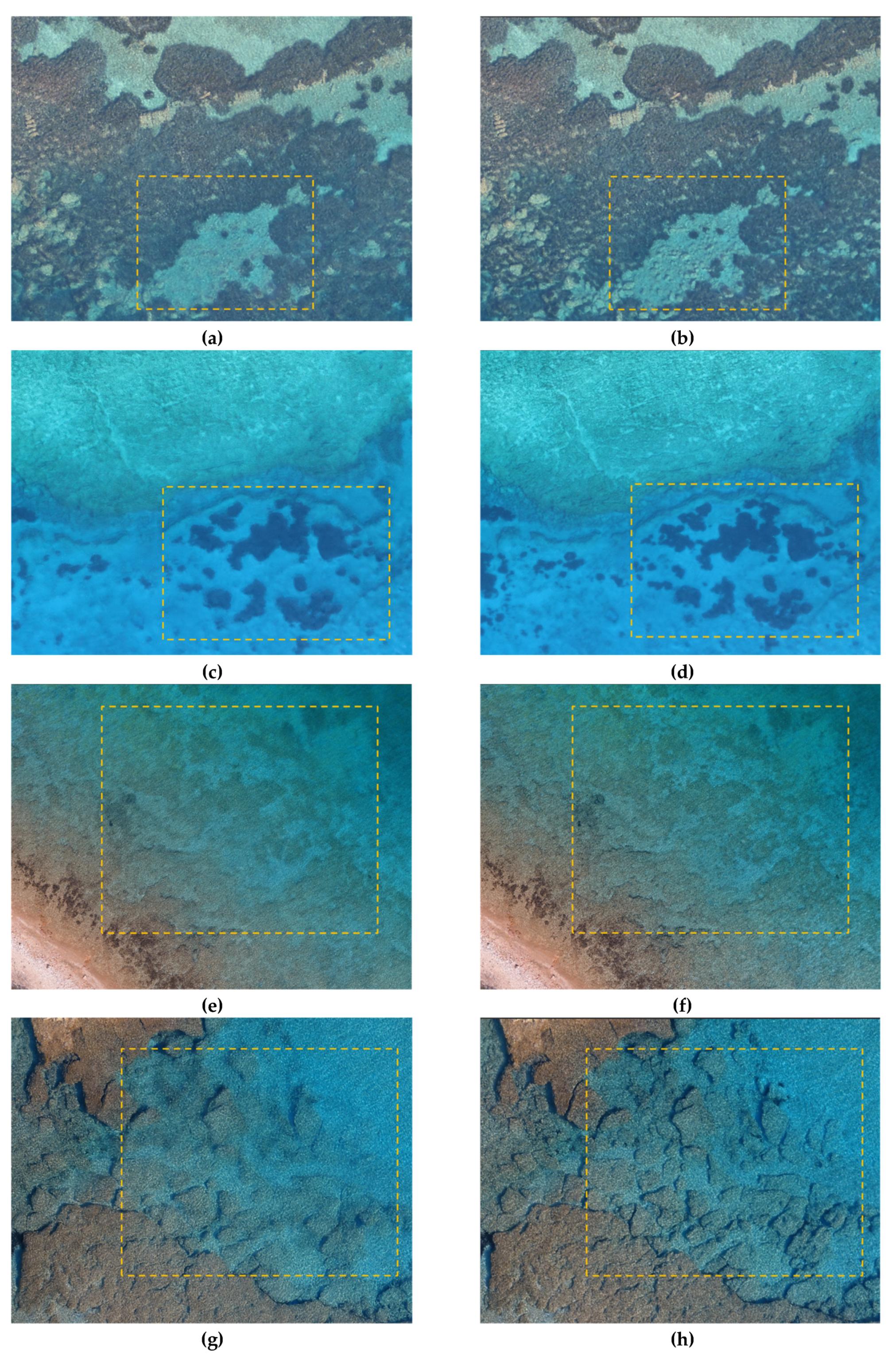
4.1. Refraction-Free Images

Figure 7a,b illustrates two example images from the Agia Napa dataset along with the corresponding refraction-free ones (d) and (e). In a similar way, Figure 7c illustrates an original image from the Amathounta test site together with the corresponding refraction-free image (f). Since cmixed is by default larger than cair in all depth cases because nwater > nair, an overall image shrinkage occurred, hence raw information were kept within the initial image frame, while areas with missing information due to shrinkage were kept black. This can be observed in Figure 7d–f zoomed areas. In Figure 7g–i, the differences between the respective images of the first and the second row are illustrated.
By observing the corrected and initial imagery, one could notice that differences are only apparent in underwater regions and that these differences are increasing with depth (from right to left, for all the images in Figure 7) as expected. Moreover, in all cases (Figure 7g–i), there is a small circular area (red dotted circle) in the nadiral point of each image, and, around it, the refraction effect is minimal. This area is bigger as the depth of the imaged seabed decreases (from the left image to the right image) since the effect of refraction is less in shallow areas than in deeper areas. This is also explained by the nature of the refraction phenomenon on the imagery [6,23]. Indeed, it behaves like a radial shift, taking into account the central projection image formation model. The center of this area of the image, having almost no refraction, is the nadiral point of the image. This area of the image is created by light rays that are characterized by a very small incidence angle (Figure 6), which, according to Snell’s law, leads to a very small refraction angle (Figure 6). Moreover, assuming a flat air-water interface and a perfectly perpendicular optical axis, the light ray that matches with the nadiral axis has a zero angle of incidence and thus is not affected by the refraction phenomenon. However, the latter is never achieved in a real-world dataset, such as the ones used here. On the contrary, the amount of correction and thus the differences between the images are increasing as the distance from the image center increases, since the amount of refraction is more intense for light rays captured far from the image center.

4.2. Assessing Quantitatively the Improvements on the SfM Results

A well-established methodology for evaluating SfM performance is to compare the sparse point cloud to some ground truth with the same data representation [37]. Towards this end, and taking into account that for the image correction approach a corrected dense point cloud was used, there is no need to evaluate the dense point cloud again, the comparison of the sparse point clouds with LiDAR ground truth data was performed for the Amathounta and Agia Napa test site, demonstrating the positive effect of the image correction on the accuracy of the results and the performance of the image correction approach. For the Cyclades-1 and Cyclades-2 test areas, since LiDAR data were not available, comparisons performed using checkpoints measured with a Total Station (an electronic/optical instrument used for surveying) on-site and acquired together with the image data. Together with the sparse point cloud produced by the corrected data, results from four state of the art refraction correction algorithms are presented and evaluated.

4.2.1. Ground Truth Data

LiDAR point clouds of the submerged areas and Total Station points were used for evaluating the developed methodology. The LiDAR point clouds were generated with the Leica HawkEye III (Leica Geosystems AG, Heerbrugg, Switzerland), a deep penetrating bathymetric airborne LiDAR system. This system includes an up to 500 kHz infrared channel (1064 nm) for topographic applications, a 10 kHz bathymetric channel (532 nm) for high accuracy and high data density for deep water, and a 35 kHz bathymetric channel optimized for shallow water and the transition zone towards the shore [38]. Table 2 presents the details of the ground truth data used.
Even though the specific LiDAR system can produce point clouds with accuracy of 0.02 m in topographic applications according to the manufacturers, when it comes to bathymetric applications, the system’s range error is in the order of ±0.15 m for depths up to 1.5 Secchi depths [38], similar to other conventional topographic airborne scanners. Regarding the Total Station points, a realistic nominal bathymetric accuracy could be estimated to be 0.05 m, taking also into account the penetration of the pole into the seabed.

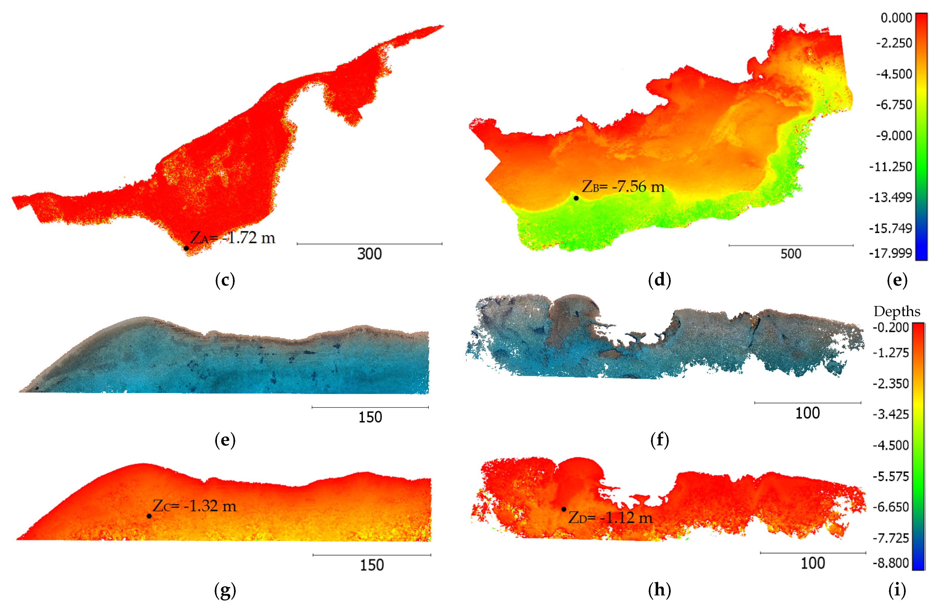
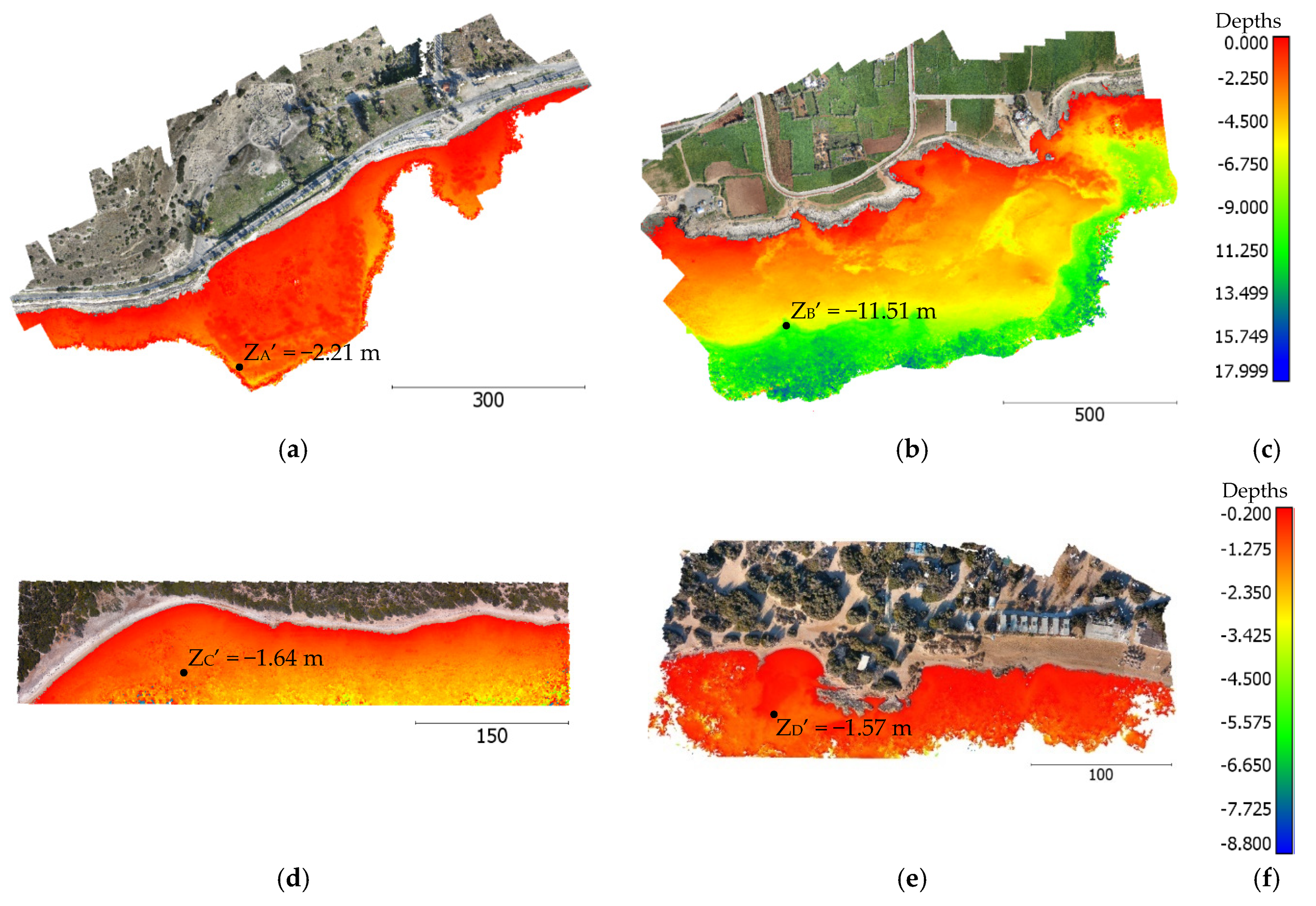
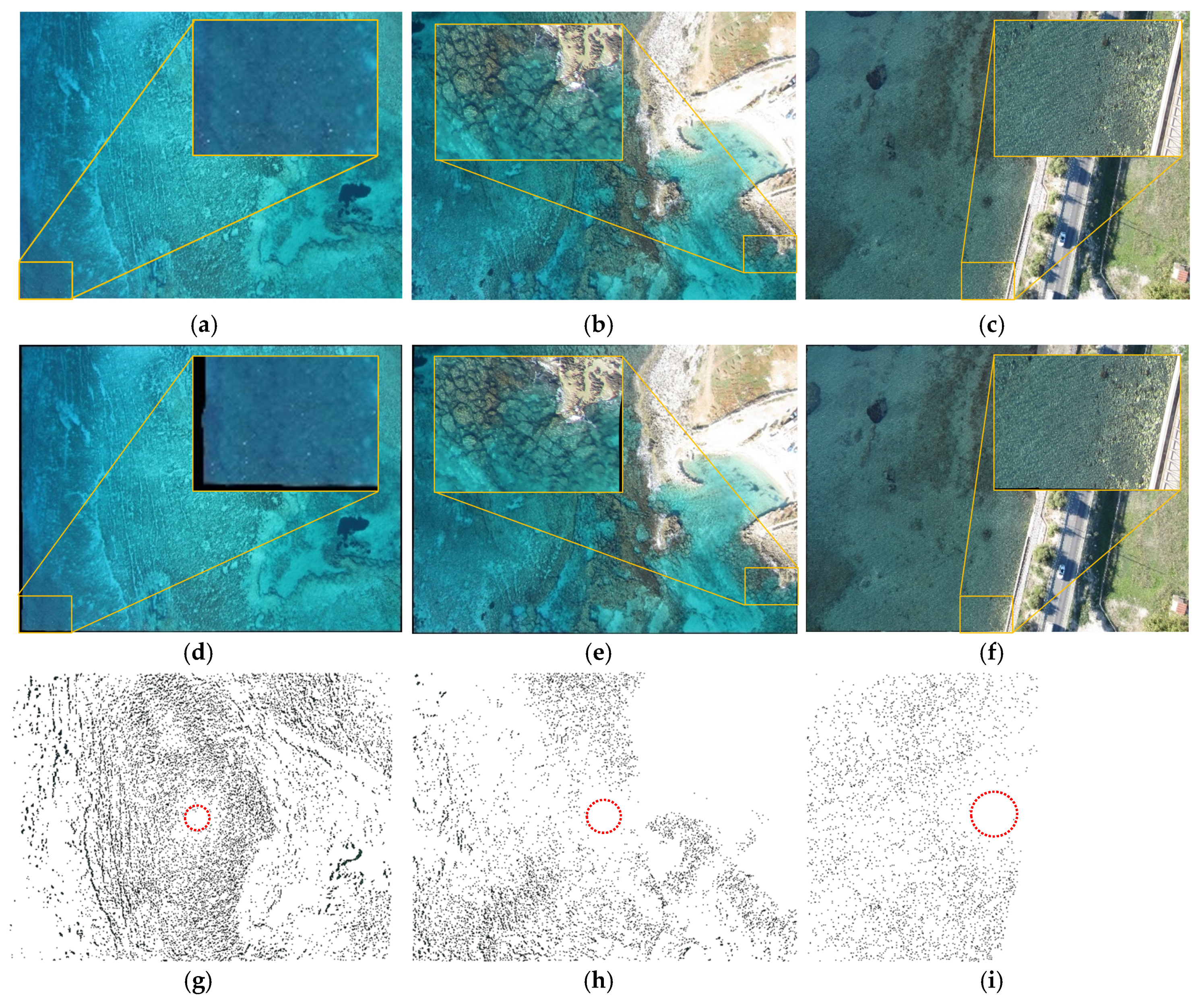
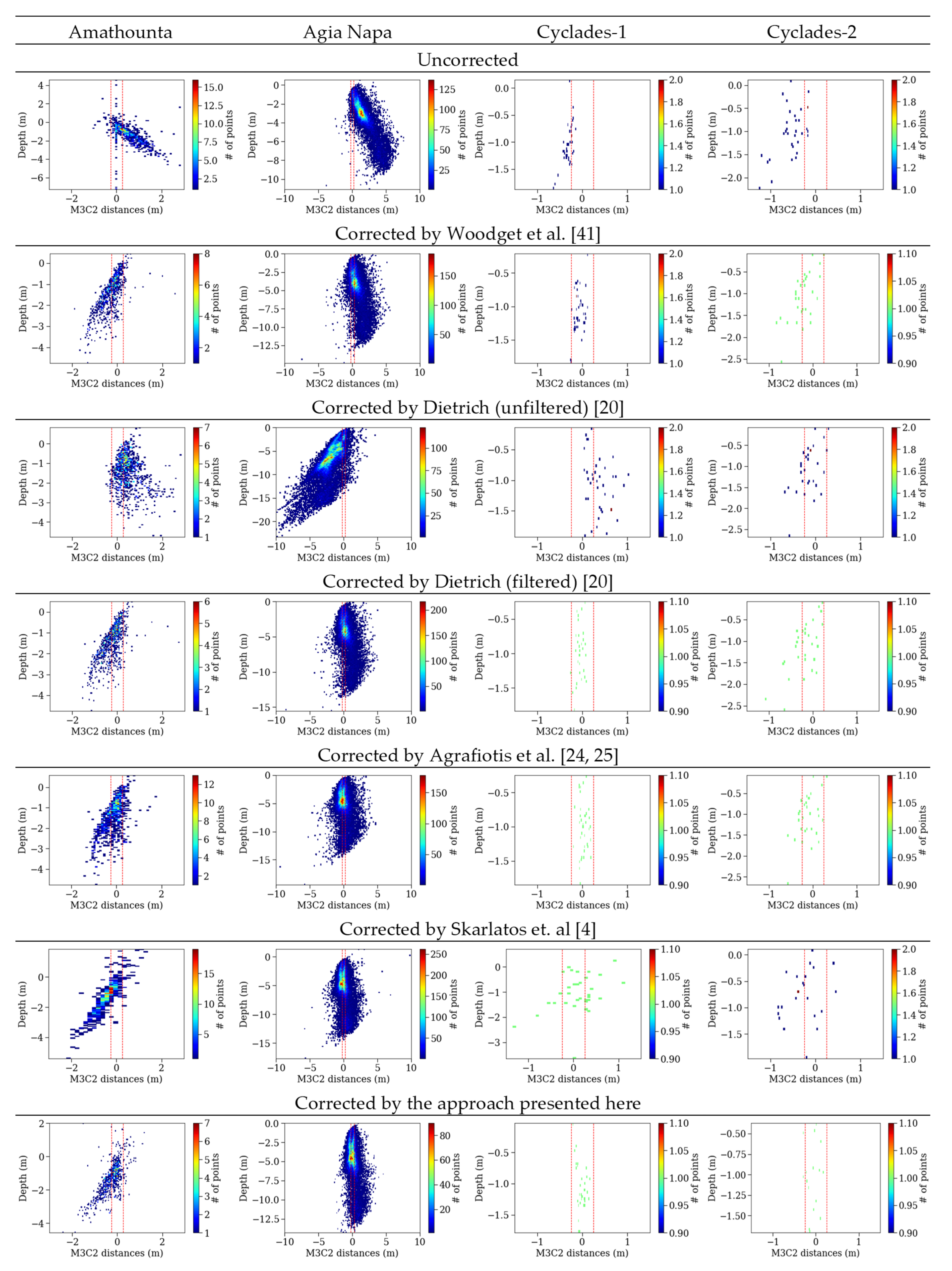
4.2.2. Qualitative and Quantitative Assessment on the Produced Sparse Point Clouds

Since the dense point cloud regeneration after the correction of the imagery is not necessary, and there is no ground truth for the exterior orientations of the cameras, to evaluate the results of the proposed image correction methodology, the sparse point clouds of the updated SfM solution were evaluated. To that end, the sparse point clouds generated using the initial imagery, and the sparse point clouds resulted from the corrected imagery using the proposed methodology were compared with the LiDAR point clouds or the Total Station points using the Multiscale Model to Model Cloud Comparison (M3C2) [39] module in Cloud Compare freeware [40] to demonstrate the changes and the differences produced by our image correction approach. The M3C2 algorithm offers accurate surface change measurement that is independent of point density [39]. Additionally and in order to stress out the accuracy of the presented methodology compared with some state of the art refraction correction approaches, the ground truth point clouds of the four test areas were compared with the sparse point clouds resulted from the image-based refraction correction approach, described in [4], and 3D space correction approaches [20,24,25,41]. Since the methodology delivered by the authors in [24,25] is already described in Section 1.1, the rest of the refraction correction methodologies are described in the following paragraph.
Authors in [41] presented a relatively simple approach for refraction correction of bathymetric elevation models using a small angle approximation. There, Snell’s Law was applied to the river bed surface to increase the apparent water depths by a multiplier of 1.34 (i.e., the refractive index of clear water) to account for the effects of refraction. The refraction correction is calculated by assuming that the angles i and r (Figure 6) are less than 10°. In [20], a more sophisticated multi-angle refraction correction approach was proposed. This author used the 3D dense point clouds and applied an iterative refraction correction method based on the positions and view angles of all the cameras used within the photogrammetric reconstruction of the position of each point in the cloud. In this article, for applying the methods described in [41] and [20], the python script delivered by the authors was used [42]. Regarding the parameters used for filtering the depth values produced by [20], a maximum angle of 35° and a maximum distance of 110 m were selected for Amathounta test site, for Agia Napa test site, a maximum angle of 35° and a maximum distance of 220 m were selected, for Cyclades-1 test site, a maximum angle of 35° and a maximum distance of 95 m were selected, while for Cyclades-2 test site, a maximum angle of 35° and a maximum distance of 85 m were selected.
In Figure 8 (first row), it could be observed that the distances between the reference data and the original image-based point clouds increase in proportion to the depth. In all the test cases demonstrated in the first row of Figure 8, the Gaussian mean of the differences ( x ¯ ) was significant. It reached 0.67 m in the Amathouda test site, 1.71 m in the Agia Napa test site, 0.32 m in Cyclades-1 test site, and 0.54 m in Cyclades-2 test site (Table 3). These comparisons clarified that the refraction effect cannot be ignored in seabed mapping applications using low altitude aerial imagery. The dashed lines in red represent the accuracy limits generally accepted for hydrography, as introduced by the International Hydrographic Organization (IHO) [43]. As could be observed in the first row of Figure 8, the majority of the points in both areas are far from the red dashed lines representing these accuracy limits. The last row of Figure 8 presents the histograms of the cloud to cloud distances (M3C2) between the ground truth and the sparse point clouds produced from corrected imagery of the image correction approach presented in this paper.
The second, third, fourth, fifth, and sixth rows of Figure 8 illustrate the comparison results between the ground truth and the sparse point clouds produced by [41], [20] (filtered in fourth and unfiltered in third), [24,25], and [4], respectively. Table 3 presents the results of all the tests performed. Both in Figure 8 and Table 3, a great improvement in the sparse point clouds, and thus the SfM accuracy, was achieved by the approach of this paper compared with the uncorrected ones. More specifically, in Amathounta test site, the initial 0.67 m mean distance was reduced to −0.19 m, in Agia Napa test site, the initial 1.71 m mean distance was reduced to −0.04 m, in Cyclades-1, the 0.32 m initial mean distance was reduced to −0.02 m, while in Cyclades-2, the 0.54 m initial mean distance was reduced to −0.06 m, including outlier points, such as seagrass, that were not captured in the ground truth clouds for all the cases or were caused due to point cloud noise again in areas with seagrass or poor texture. It is also important to stress out here that the results of the proposed approach outperformed the results of the image-based iterative approach presented in [4] in these test sites. For all the test sites, the resulting mean distances in the sparse point cloud met and exceeded the accuracy standards generally accepted for hydrography, as introduced by the International Hydrographic Organization (IHO), where in its simplest form, the vertical accuracy requirement for shallow water hydrography can be set as a total of ±25 cm (one sigma) from all sources, including tides [43].
Compared with the results of the rest of the tested refraction correction approaches, for all the tested areas, the approach presented by Agrafiotis et al., in [24,25], outperformed the rest. This result also justifies the selection of this approach for the correction of the dense point clouds before the DSM generation. Compared with the accuracy levels reached by Agrafiotis et al., in [24,25], the approach presented here reached the same levels of accuracy in Agia Napa, Cyclades-1, and Cyclades-2 test sites, while in Amathounta, results were not of the same accuracy; however, they still met the standards of IHO [43]. However, [24,25] did not deliver corrected image data but only point clouds, thus being less useful when image products are required. The difference in the performance of the presented approach is explained in Section 4.5. Regarding the rest of the compared refraction correction approaches, both [20] and [41] were developed for correcting the effects of refraction on shallow water riverbeds, and they seemed to produce quite accurate and reliable results, especially when filtering was applied in [20]. The improved accuracy of the proposed image correction approach could be explained by the fact that the already available approaches [20] and [41] are using the camera positions and the point clouds that are produced using the refracted imagery, which affects SfM and MVS processes and degrades the results. Regarding the approach presented in [24,25], this method is also correcting point clouds generated by the refracted imagery, but not exploiting the interior and exterior orientations of the camera, as done in [20] and [41], and thus is less affected by those. The approach presented here, by correcting the imagery from refraction, seems to overcome the transferred errors from the initial orientations, because the SfM results are being updated, delivering a more accurate geometry of the block and more accurate SfM results.

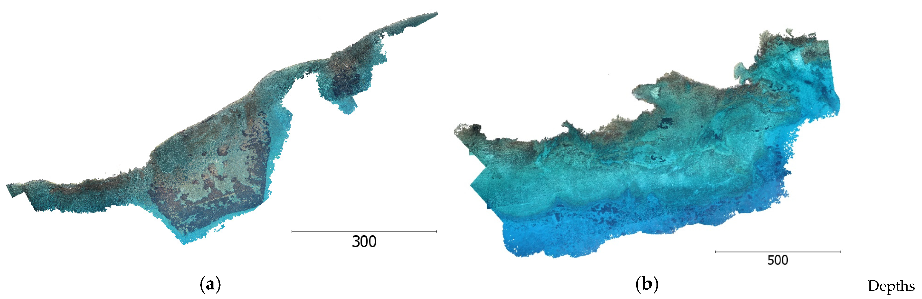
4.3. Assessing Qualitatively the Improvements on the Textured Seabed Models

Figure 9 illustrates parts of the textured 3D models of Amathounta, Agia Napa, Cyclades-1, and Cyclades-2 test sites. There, a textured model created by a mesh, produced using the refraction corrected point cloud, and the original uncorrected imagery is presented in the left column in order to highlight that when textured models are needed, the correction of the seabed point cloud and the mesh is not enough and image correction is also needed. In Figure 9 (right column), the textured model created using the mesh, produced using the refraction corrected point cloud, and the corrected imagery using the proposed approach is presented. By comparing these results, it is clearly obvious (especially in the areas inside the orange dashed rectangle) that the details of the seabed on the textured model created using the uncorrected imagery are degraded, especially when depth increases (Figure 9c–d) or presents detailed rock formations with abrupt changes in elevation (Figure 9b–d) and Figure 9g–h). This leads to a significant loss of information on the textured 3D model and to an unreliable representation of the seabed, highlighting the critical need to correct the original dataset from refraction and update the SfM solution. At the same time, as can be observed in Figure 9e,f, dry land areas are remaining unchanged, highlighting the effects of the refraction on the reliability of the created models of the seabed.

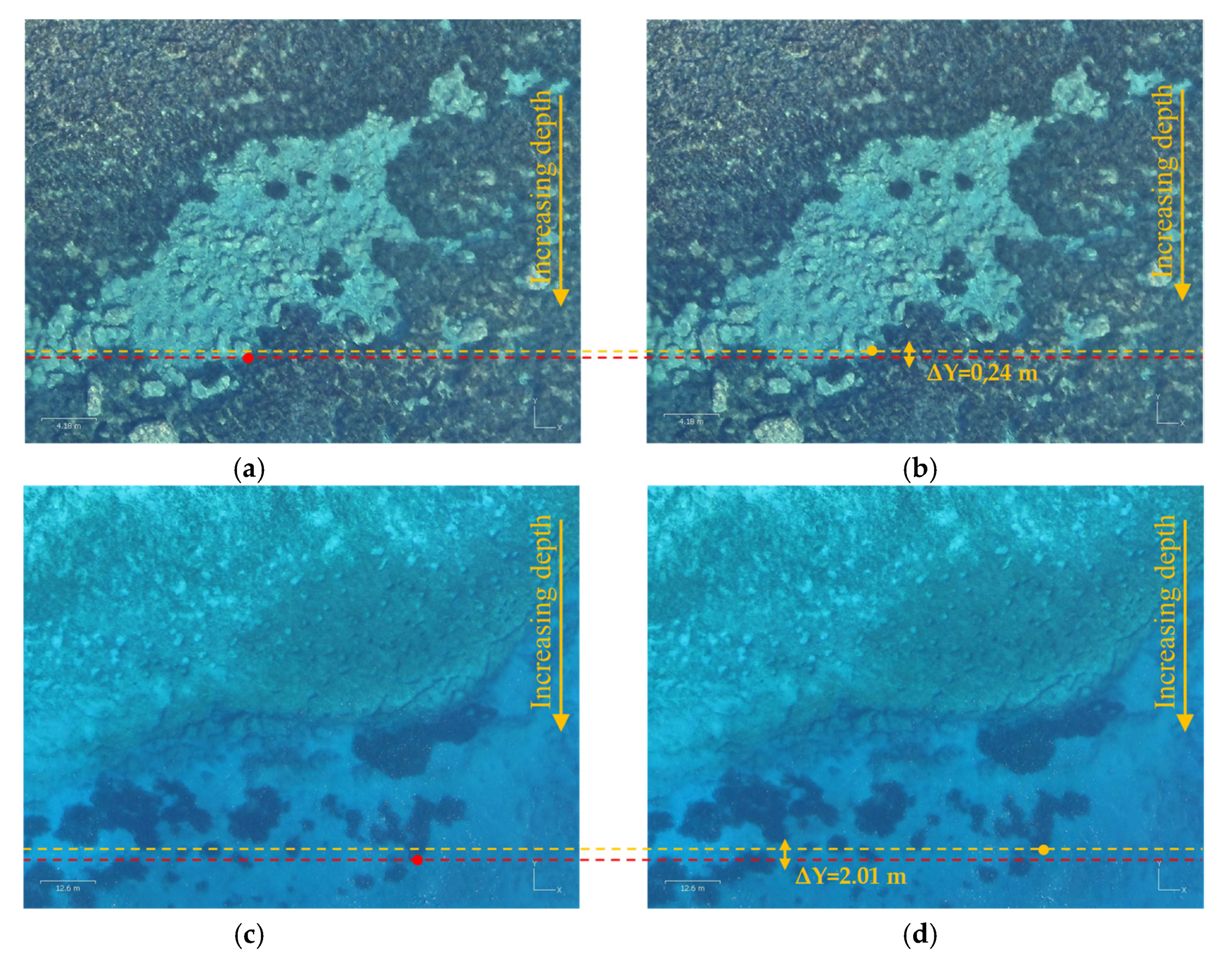
4.4. Assessing Quantitatively the Improvements on the Orthoimages

Figure 10 illustrates parts of the orthoimages of Amathounta, Agia Napa, Cyclades-1, and Cyclades-2 test sites. Orthoimages created using the merged DSM and the original imagery are presented in the left column, while in the right column, orthoimages using the merged DSM and the corrected imagery are presented. Dashed lines are used to facilitate the comparison between the left and the right column; red dashed lines pass from the red dots, which represent a specific point in the orthoimage of each test site produced using the uncorrected imagery. The orange dashed line passes from the orange dots, which represent the same specific point (being in red in the left column) in the orthoimage of each test site produced using the corrected imagery. The horizontal displacements of the marked points on the orthoimages are reported also in Figure 10. Contrarywise to the textured 3D models (Figure 9), in the orthoimages, no important qualitative differences can be spotted. However, remarkable horizontal differences can be found in the direction that the depth increases. In more detail, in the Amathounta test site (Figure 10a,b), where the GSD of the orthoimage was 3.64 cm/pix, differences of 5–8 pixels can be spotted in an average depth of 1.60 m, leading to horizontal errors of 18.2 cm–29.12 cm. In the Agia Napa test site (Figure 10c,d), where the GSD of the orthoimage was 7.72 cm/pix, differences of 23–26 pixels can be spotted in a depth of 13.80 m, leading to horizontal errors of 177.5 cm–200.7 cm. In the Cyclades-1 test site (Figure 10e,f), where the GSD of the orthoimage was 3.08 cm/pix, differences of 18–21 pixels can be spotted in a depth of 2.24 m, leading to horizontal errors of 55.4 cm–64.7 cm. Finally, in the Cyclades-2 test site (Figure 10g,h), where the GSD of the orthoimage was 2.01 cm/pix, differences of 6–17 pixels can be spotted in a depth of 1.98 m, leading to horizontal errors of 12.06 cm–34.17 cm.
Results suggested that when depth increases, horizontal errors on the orthoimages are increasing if no refraction corrections are applied to the images. In shallow areas, these errors might not be obvious. However, in deeper areas, such as Agia Napa (Figure 10c,d), Cyclades-1 (Figure 10e,f), and Cyclades-2 (Figure 10g,h), the horizontal differences are evident and very important. The magnitude of these errors depends on the depth error and the position of the point on the image. These differences cannot be neglected for accurate seabed representation in an orthoimage. Consequently, the refraction correction of the imagery to be used for the orthoimage generation is necessary even if a correct DSM of the seabed is available.

4.5. Error Propagation within the Sequential Steps of the Proposed Approach

In this subsection, certain factors that affect the overall accuracy of the produced refraction-free images are discussed. In order to estimate the effect and the amount of error that propagates, the corrected dense point clouds were compared with their respective ground truth point clouds, described in detail in Section 4.2.1. For the Amathounta test site, the mean M3C2 distance [39] between the compared dense point clouds reached 0.03 m with a standard deviation of 0.35 m; for the Agia Napa test site, the mean M3C2 distance was calculated as 0.085 m with a standard deviation of 0.49 m; for the Cyclades-1 test site, the mean M3C2 distance was calculated as −0.01 m with a standard deviation of 0.09 m; while for the Cyclades-2 test site, the mean M3C2 distance was calculated as −0.01 m with a standard deviation of 0.31 m.
To evaluate the effect of these errors in the image correction procedure, through their use in the merged DSM creation, two examples are provided with a seabed point A laying at 5 m depth at the Amathounta and Agia Napa datasets. In particular, taking into account that the average flying height for Amathounta dataset was 103 m and for Agia Napa 209 m, the following can be calculated:
For the Amathounta test site, point A is having a real depth 5 m and a calculated depth of 5.03 m (real depth plus the mean distance computed by M3C2). Then, the c mixed for the real depth and the c mixed for the calculated depth can be computed using Equation (3);
c mixed =   ( P air   n air   +   P water   n water )   c air = ( 0.9537037037037037   1   +   0.04629629629629628   1.34 )   2827.05   =   2871.55   pixels
c mixed =   ( P air   n air   +   P water   n water )   c air = ( 0.9534388595760437   1   +   0.046561140423956315   1.34 )   2827.05   =   2871.80   pixels
The difference between c mixed   a n d   c mixed was calculated:
Δ c mixed = c mixed c mixed =   0.25   pixels
To compute the effect of this difference in the image coordinates of points a and a’ that are the projections of the non-refracted and the refracted ray coming from seabed point A, respectively, two different radial distances were considered for testing: 100 pixels and 1500 pixels.
For a point a having radial distance r 100 pixels;
r c mixed = 101.574   pixels   and   r c mixed =   101.583   pixels ,   Δ r c mixed = 0.009   pixels
For a point a having radial distance r 1500 pixels;
r c mixed = 1523.61   pixels   and   r c mixed =   1523.75   pixels ,   Δ r c mixed = 0.160   pixels
For the same point in Agia Napa test site having a real depth 5 m and a calculated depth of 5.085 m (real depth plus the mean distance computed by M3C2), the c mixed for the real depth and the c mixed for the calculated depth were calculated using Equation (3);
c mixed =   ( P air   n air   +   P water   n water )   c air = ( 0.97663551401869161   +   0.02336448598130836   1.34 )   2852.34 =   2874.99   pixels
c mixed =   ( P air   n air   +   P water   n water )   c air = ( 0.9762477520610972   1   +   0.02375224793890285   1.34 )   2852.34   =   2875.37   pixels
The difference between c mixed   a n d   c mixed was calculated:
Δ c mixed = c mixed c mixed =   0.37   pixels
To compute the effect of this difference in the image coordinates of points a and a’ that are the projections of the non-refracted and the refracted ray coming from seabed point A, respectively, two different radial distances were considered for testing: 100 pixels and 1500 pixels.
For a point a having radial distance r 100 pixels;
r c mixed = 100.794   pixels   and   r c mixed =   100.808   pixels ,   Δ r c mixed = 0.014   pixels
For a point a having radial distance r 1500 pixels;
r c mixed = 1511.92   pixels   and   r c mixed =   1512.11   pixels ,   Δ r c mixed = 0.19   pixels
In the tests performed above, the differences observed between c mixed c mixed and r c mixed r c mixed when adding the mean distance as a constant value were considered negligible.
In addition to the aforementioned analytical estimation, Figure 11 presents the differences Δ c mixed of the c mixed calculated using the real depth and the c mixed calculated using the calculated depth of a point. Solid lines represent the Δ c mixed calculated for Amathounta (in green), Agia Napa (in blue), Cyclades-1 (in cyan for 35 m flight height and in orange for 70 m), and Cyclades-2 (in light green for 35 m flight height and in red for 70 m) by adding the mean distance calculated for each site as a constant value to the hypothetical real depth. Dashed lines represent the Δ c mixed calculated by adding the mean distance and the standard deviation, while dotted lines represent the Δ c mixed calculated by adding the mean distance minus the standard deviation. That way, the maximum Δ c mixed can be calculated for each depth.
Our results suggested that the larger the depth, the smaller the differences between c mixed and c mixed . Moreover, when the standard deviation was added, the Δ c mixed calculated for the Cyclades-2 test site with a flight height of 35 m, the c mixed was affected the most by the errors present in the DSM, even though they were smaller than the errors at the Agia Napa test site. This result can be explained by the fact that the total added error in Cyclades-2 (35 m) had a greater effect on the percentages of air and water in the total light ray distance, being shallower and having a very small flight height. Excluding this test case, which was the worst, Δ c mixed was not more than 3.5 pixels in Amathounta and Cyclades-2 (70 m) test site and no more than 2.7 pixels in Agia Napa test site, while the Δ c mixed for the Cyclades-1 test site remained below 2 pixels for all the flight heights. In the typical case, Δ c mixed was not more than 0.4 pixels for all the tested cases.
Figure 12 presents the radial distance differences Δ r c mixed in relation to the radial distance r for two different depths, 50 and 15 m, for all the test sites. Solid lines represent the Δ c mixed calculated for Amathounta (in green), Agia Napa (in blue), Cyclades-1 (in cyan for 35 m flight height and in orange for 70 m), and Cyclades-2 (in light green for 35 m flight height and in red for 70 m) by adding the mean distance calculated for each site as a constant value to the hypothetical real depth. Dashed lines represent the Δ r c mixed calculated by adding the mean distance and the standard deviation, while dotted lines represent the Δ r c mixed calculated by adding the mean distance minus the standard deviation. That way, the maximum Δ r c mixed can be calculated for each of the two tested depths. The larger the value (error) added in the real depths, the larger the radial distance differences Δ r c mixed . On the contrary, by observing the results among Figure 12a–d, the deeper the point is, the smaller the radial distance differences Δ r c mixed are. For example, in the Amathounta test site, presenting the larger differences between Figure 12a,b, the maximum Δ r c mixed calculated for the depth of 5 m was 2.2 pixels on the edge of the image and 1.9 pixels for the depth of 15 m. For the same depths, the maximum Δ r c mixed in the Agia Napa test site was calculated as 1.8 and 1.6 pixels, respectively. Coming to the typical case, Δ r c mixed reached 0.2 and 0.12 pixels in the Amathounta test site, while for the same depths in the Agia Napa test site, Δ r c mixed reached 0.25 and 0.23 pixels, respectively, for the radial distance of 2000 pixels, being the edge of the image. Coming now to Figure 12c,d that present the Δ r c mixed over the Cyclades-1 and Cyclades-2 datasets, it is obvious that the smaller the flight height, the larger the Δ r c mixed calculated, as observed also in Figure 11. For the Cyclades-1 dataset, the maximum Δ r c mixed calculated for the depth of 5 m was 1.1 pixels on the edge of the image and 0.8 pixels for the depth of 15 m and flight height of 35 m; hence for flight height of 70 m, the calculated Δ r c mixed was even smaller. For the same depths, the maximum Δ r c mixed in the Cyclades-2 test site was calculated as 4.5 and 2.8 pixels, respectively. Coming to the typical case, Δ r c mixed reached 0.18 and 0.11 pixels in the Cyclades-1 test site, while for the same depths in the Cyclades-2 test site, Δ r c mixed reached 0.22 and 0.18 pixels, respectively, for the radial distance of 2000 pixels, being the edge of the image. Again, our results suggested that the larger the depth, the smaller the differences between r c mixed and ’, since they clearly depend on the calculated c mixed . Similarly, the Amathounta and Cyclades-2 test sites were more affected when the standard deviation was added as a constant error, presenting Δ r c mixed .
Considering the results in Figure 11 and Figure 12, in the majority of the cases, the amount of the errors introduced in the DSM by the refraction correction approach that is applied on the dense point clouds is not capable of affecting the overall accuracy of the proposed approach for correcting image refraction, especially in the typical case. Subpixel errors were transferred in cases, where the mean errors applied were not affecting the image correction quality and accuracy. However, areas having larger mean M3C2 distances might exist due to the presence of seagrass and sandy bottom areas, leading to larger Δ c mixed and Δ r c mixed , and thus affecting the image correction approach. This is the reason why even the depth correction approach applied on the dense point cloud proved to be the most accurate among the ones compared in Table 3, ensuring a more accurate image refraction correction; the mean distances calculated for the proposed approach in this paper (Table 3) are always greater from the results of the method of Agrafiotis et al., in [24,25], used to correct the dense point clouds. Taking into account this and in order to translate the results Figure 11 and Figure 12 about the transferable errors in the whole process into measurable distances, the differences between the mean distances of the sparse point clouds corrected by [24,25] and the proposed approach were calculated; For Amathounta test site, it was 0.10 m; for Agia Napa test site, it was 0.01 m; for Cyclades-1 test site, it was 0.04 m, and for Cyclades-2 test site, it was 0.02 m. Considering sea level alterations, ripples, and the anaglyph of the seabed, we concluded that the amount of the errors that were propagated within the presented approach was not capable of affecting the overall accuracy of the proposed approach, being in most of the cases less than the GSD.

5. Discussion

Compared with the point clouds of the ground truth, the sparse point clouds that were produced based on the refraction-free dataset managed to achieve accuracy within the IHO standards [43], outperforming existing approaches. This finding could be explained by the fact that similar approaches [20] and [41] are using the camera positions calculated using the refracted imagery, which certainly affected the performance of SfM and MVS processes. Regarding the approach presented in [24,25], even though it is also correcting point clouds generated by the refracted imagery, it is not exploiting the interior and exterior orientations of the cameras, as done in [20] and [41], thus being less affected by those factors. Moreover, the SVR model developed in [24,25] was trained on point clouds generated using refracted imagery and, consequently, had “learned” to avoid errors introduced by the erroneous cameras positions.
On the contrary, the approach presented here, by correcting the initial imagery from refraction, overcomes the transferred errors resulting from the initial orientations, since SfM results are being updated, delivering a more accurate geometry of the block and more accurate SfM results.
By correcting the imagery for refraction effects, a variety of applications becomes possible, offering more information in addition to the standard seabed surface/anaglyph. With the proposed approach, the generation of accurate, reliable, and detailed orthoimages and textures for the seabed 3D models is achieved as an additional and very valuable deliverable for many applications. Orthoimages can be produced based on the merged DSM, the updated camera positions, and the refraction-free images. Having corrected the imagery, which is the primary source of information for all the image-based mapping applications, semantic information can be then used as a primary input to the SfM-MVS process in order to produce semantically labeled 3D point clouds. It also facilitates a wide range of exploitations of the available visual information, such as seabed classification, coral reefs monitoring, general benthic community mapping, marine litter mapping, and more.
As with any method based on imagery, limitations were imposed in areas having texture of low quality and non-static objects (e.g., sand and seagrass areas respectively) since SfM-MVS might fail in these areas. Also, for most of the cases (except small lakes that are surrounded by land), the unfavorable position of the GCPs in the photogrammetric block situated on the shore might also compromise the accuracy of the block and the point cloud, respectively, in the deeper areas of the seabed that are far from the GCPs. Additionally, favorable conditions, such as clear water, calm water surface, and bottom texture, are required in order to improve the results of the SfM-MVS processing and eliminate the noise of the generated image-based point cloud. Areas having larger mean M3C2 distances may remain due to the presence of factors like the aforementioned ones, thus affecting the image correction approach following the already described error propagation chain. However, in the majority of the cases, the amount of the errors introduced in the merged DSM is not capable to affect the overall accuracy of the proposed approach, when optimal flight, visibility, and wave conditions apply.

6. Conclusions

A new approach for correcting the effects of water refraction on aerial imagery was presented in this study. This approach first exploits DepthLearn [24,25], a recent machine learning procedure that can recover depth on the derived dense point clouds, and then corrects the refraction effect on the original imaging dataset, exploiting image transformation and resampling techniques. That way, the operational SfM and MVS processing pipelines are ultimately executed on a refraction-free set of aerial datasets, resulting in highly accurate bathymetric maps. At the same time, this approach allows for robust, cost-effective mapping of the coastal zone, both land and sea bottom, for image and dense point cloud deliverables.
The developed approach was tested and validated over four different test sites in Greece and Cyprus having different flight plans, different UAV systems, different sensors, but the same optimal weather conditions. A qualitative evaluation of the proposed approach was performed through the visual assessment of the textured models created by the merged DSM and the original uncorrected imagery and the textured models created by the merged DSM and refraction-free imagery. Results suggested a great improvement in the detail and the quality of the textured 3D models when the results of the proposed approach are used. The quantitative evaluation was performed through a comparison of the sparse point clouds produced after the corrected imagery with ground truth points and through a comparison between orthoimages created by the merged DSM and the original uncorrected imagery and orthoimages created by the merged DSM and refraction-free imagery. Results suggested that the proposed refraction correction approach produces refraction-free images in a very accurate and reliable way, outperforming existing approaches. Also, when these refraction-free images are used, more accurate and reliable orthoimages of the seabed can be generated. For all the test sites, the proposed method met and exceeded the accuracy standards generally accepted for hydrography, as introduced by the International Hydrographic Organization (IHO), where in its simplest form, the vertical accuracy requirement for shallow water hydrography can be set as a total of ±25 cm (one sigma) from all sources, including tides [43].

Author Contributions

Conceptualization, P.A. and D.S.; methodology, P.A. and D.S.; software, P.A., D.S.; validation, P.A., K.K., D.S., and A.G.; formal analysis, P.A. and K.K.; investigation, P.A., D.S., and K.K.; resources, P.A. and D.S.; data curation, P.A. and D.S.; writing—original draft preparation, P.A.; writing—review and editing, P.A., D.S., A.G., and K.K. All authors have read and agreed to the published version of the manuscript.

Funding

This research received no external funding

Acknowledgments

Authors would like to acknowledge the Dep. of Land and Surveys of Cyprus for providing the LiDAR reference data, the Cyprus Dep. of Antiquities for permitting the flight over the Amathouda site and commissioning the flight over Agia Napa, the underwater archaeologist Ioanna Kraounaki and the Ephorate of Underwater Antiquities of Greece for commissioning the flights over Cyclades datasets, Rural and Surveying Engineer Dimitrios Kontos of Topodomiki S.A. for conducting the flights of Cyclades datasets, and Honor Frost Foundation for partially funding the research in Cyprus’ datasets.

Conflicts of Interest

The authors declare no conflict of interest.

References

  1. Agrafiotis, P.; Skarlatos, D.; Forbes, T.; Poullis, C.; Skamantzari, M.; Georgopoulos, A. Underwater Photogrammetry in Very Shallow Waters: Main Challenges and Caustics Effect Removal. Int. Arch. Photogramm. Remote Sens. Spat. Inf. Sci. 2018, XLII-2, 15–22. [Google Scholar] [CrossRef] [Green Version]
  2. Karara, H.M. Non-Topographic Photogrammetry, 2nd ed.; American Society for Photogrammetry and Remote Sensing: Falls Church, VA, USA, 1989. [Google Scholar]
  3. Kasvi, E.; Salmela, J.; Lotsari, E.; Kumpula, T.; Lane, S.N. Comparison of remote sensing based approaches for mapping bathymetry of shallow, clear water rivers. Geomorphology 2019, 333, 180–197. [Google Scholar] [CrossRef]
  4. Skarlatos, D.; Agrafiotis, P. A Novel Iterative Water Refraction Correction Algorithm for Use in Structure from Motion Photogrammetric Pipeline. J. Mar. Sci. Eng. 2018, 6, 77. [Google Scholar] [CrossRef] [Green Version]
  5. Green, E.; Mumby, P.; Edwards, A.; Clark, C. Remote Sensing: Handbook for Tropical Coastal Management; United Nations Educational, Scientific and Cultural Organization (UNESCO): Paris, France, 2000. [Google Scholar]
  6. Georgopoulos, A.; Agrafiotis, P. Documentation of a Submerged Monument Using Improved Two Media Techniques. In Proceedings of the 2012 18th International Conference on Virtual Systems and Multimedia, Milan, Italy, 2–5 September 2012; pp. 173–180. [Google Scholar] [CrossRef]
  7. Butler, J.B.; Lane, S.N.; Chandler, J.H.; Porfiri, E. Through-water close range digital photogrammetry in flume and field environments. Photogramm. Rec. 2002, 17, 419–439. [Google Scholar] [CrossRef]
  8. Tewinkel, G.C. Water depths from aerial photographs. Photogramm. Eng. 1963, 29, 1037–1042. [Google Scholar]
  9. Shmutter, B.; Bonfiglioli, L. Orientation problem in two-medium photogrammetry. Photogramm. Eng. 1967, 33, 1421–1428. [Google Scholar]
  10. Maas, H.-G. On the Accuracy Potential in Underwater/Multimedia Photogrammetry. Sensors 2015, 15, 18140–18152. [Google Scholar] [CrossRef]
  11. Wang, Z. Principles of Photogrammetry (with Remote Sensing); Publishing House of Surveying and Mapping: Beijing, China, 1990. [Google Scholar]
  12. Shan, J. Relative orientation for two-media photogrammetry. Photogramm. Rec. 1994, 14, 993–999. [Google Scholar] [CrossRef]
  13. Fryer, J.F. Photogrammetry through shallow waters. Aust. J. Geod. Photogramm. Surv. 1983, 38, 25–38. [Google Scholar]
  14. Elfick, M.H.; Fryer, J.G. Mapping in shallow water. Int. Arch. Photogramm. Remote Sens. 1984, 25, 240–247. [Google Scholar]
  15. Ferreira, R.; Costeira, J.P.; Silvestre, C.; Sousa, I.; Santos, J.A. Using Stereo Image Reconstruction to Survey Scale Models of Rubble-Mound Structures. In Proceedings of the First International Conference on the Application of Physical Modelling to Port and Coastal Protection, Porto, Portugal, 8–10 May 2006. [Google Scholar]
  16. Muslow, C. A flexible multi-media bundle approach. Int. Arch. Photogramm. Remote Sens. Spat. Inf. Sci. 2010, 38, 472–477. [Google Scholar]
  17. Wolff, K.; Forstner, W. Exploiting the multi view geometry for automatic surfaces reconstruction using feature based matching in multi media photogrammetry. IAPRS 2000, 33, 900–907. [Google Scholar]
  18. Ke, X.; Sutton, M.A.; Lessner, S.M.; Yost, M. Robust stereo vision and calibration methodology for accurate three-dimensional digital image correlation measurements on submerged objects. J. Strain Anal. Eng. Des. 2008, 43, 689–704. [Google Scholar] [CrossRef]
  19. Byrne, P.M.; Honey, F.R. Air Survey and Satellite Imagery Tools for Shallow Water Bathymetry. In Proceedings of the 20th Australian Survey Congress, Darwin, Australia, 20 May 1977; pp. 103–119. [Google Scholar]
  20. Dietrich, J.T. Bathymetric Structure-from-Motion: Extracting shallow stream bathymetry from multi-view stereo photogrammetry. Earth Surf. Process. Landf. 2017, 42, 355–364. [Google Scholar] [CrossRef]
  21. Murase, T.; Tanaka, M.; Tani, T.; Miyashita, Y.; Ohkawa, N.; Ishiguro, S.; Suzuki, Y.; Kayanne, H.; Yamano, H. A photogrammetric correction procedure for light refraction effects at a two-medium boundary. Photogramm. Eng. Remote Sens. 2008, 74, 1129–1136. [Google Scholar] [CrossRef]
  22. Mandlburger, G. Through-Water Dense Image Matching for Shallow Water Bathymetry. Photogramm. Eng. Remote Sens. 2019, 85, 445–455. [Google Scholar] [CrossRef]
  23. Agrafiotis, P.; Georgopoulos, A. Camera Constant In The Case Of Two Media Photogrammetry. Int. Arch. Photogramm. Remote Sens. Spatial Inf. Sci. 2015, 40, 1–6. [Google Scholar] [CrossRef] [Green Version]
  24. Agrafiotis, P.; Skarlatos, D.; Georgopoulos, A.; Karantzalos, K. Shallow Water Bathymetry Mapping From UAV Imagery Based On Machine Learning. Int. Arch. Photogramm. Remote Sens. Spat. Inf. Sci. 2019, XLII-2/W10, 9–16. [Google Scholar] [CrossRef] [Green Version]
  25. Agrafiotis, P.; Skarlatos, D.; Georgopoulos, A.; Karantzalos, K. DepthLearn: Learning to Correct the Refraction on Point Clouds Derived from Aerial Imagery for Accurate Dense Shallow Water Bathymetry Based on SVMs-Fusion with LiDAR Point Clouds. Remote Sens. 2019, 11, 2225. [Google Scholar] [CrossRef] [Green Version]
  26. Okamoto, A. Wave influences in two-media photogrammetry. Photogramm. Eng. Remote Sens. 1982, 48, 1487–1499. [Google Scholar]
  27. Fryer, J.G.; Kniest, H.T. Errors in Depth Determination Caused by Waves in Through-Water Photogrammetry. Photogramm. Rec. 1985, 11, 745–753. [Google Scholar] [CrossRef]
  28. Harwin, S.; Lucieer, A.; Osborn, J. The Impact of the Calibration Method on the Accuracy of Point Clouds Derived Using Unmanned Aerial Vehicle Multi-View Stereopsis. Remote Sens. 2015, 7, 11933–11953. [Google Scholar] [CrossRef] [Green Version]
  29. Rusu, R.B.; Cousins, S. 3d Is Here: Point Cloud Library (PCL). In Proceedings of the 2011 IEEE International Conference on Robotics and Automation, Shanghai, China, 9–13 May 2011; pp. 1–4. [Google Scholar]
  30. Brown, D.C. Lens distortion for close-range Photogrammetry. P. Eng. 1971, 37, 855–866. [Google Scholar]
  31. Brown, D.C. Calibration of close range cameras. Int. Arch. Photogram. 1972, 19. [Google Scholar]
  32. Mullen, R. Manual of Photogrammetry; ASPRS Publications: Bethesda, MD, USA, 2004. [Google Scholar]
  33. Quan, X.; Fry, E. Empirical equation for the index of refraction of seawater. Appl. Opt. 1995, 34, 3477–3480. [Google Scholar] [CrossRef] [PubMed]
  34. Green, P.J.; Sibson, R. Computing Dirichlet tessellations in the plane. Comput. J. 1978, 21, 168–173. [Google Scholar] [CrossRef] [Green Version]
  35. Goshtasby, A.A. Piecewise linear mapping functions for image registration. Pattern Recognit. 1986, 19, 459–466. [Google Scholar] [CrossRef]
  36. Goshtasby, A.A. 2-D and 3-D Image Registration: For Medical, Remote Sensing, and Industrial Applications; John Wiley & Sons: Hoboken, NJ, USA, 2005. [Google Scholar]
  37. Bianco, S.; Ciocca, G.; Marelli, D. Evaluating the performance of structure from motion pipelines. J. Imaging 2018, 4, 98. [Google Scholar] [CrossRef] [Green Version]
  38. Leica HawkEye, III. Available online: https://leica-geosystems.com/-/media/files/leicageosystems/products/datasheets/leica_hawkeye_iii_ds.ashx?la=en (accessed on 7 August 2019).
  39. Lague, D.; Brodu, N.; Leroux, J. Accurate 3D comparison of complex topography with terrestrial laser scanner: Application to the Rangitikei canyon (NZ). ISPRS J. Photogramm. Remote Sens. 2013, 82, 10–26. [Google Scholar] [CrossRef] [Green Version]
  40. CloudCompare (Version 2.11 Alpha) [GPL Software]. Available online: http://www.cloudcompare.org/ (accessed on 15 July 2019).
  41. Woodget, A.S.; Carbonneau, P.E.; Visser, F.; Maddock, I.P. Quantifying submerged fluvial topography using hyperspatial resolution UAS imagery and structure from motion photogrammetry. Earth Surf. Process. Landf. 2015, 40, 47–64. [Google Scholar] [CrossRef] [Green Version]
  42. Dietrich, J.T. pyBathySfM v4.0; GitHub: San Francisco, CA, USA, 2019; Available online: https://github.com/geojames/pyBathySfM (accessed on 24 October 2019).
  43. Guenther, G.C.; Cunningham, A.G.; LaRocque, P.E.; Reid, D.J. Meeting the Accuracy Challenge in Airborne Bathymetry; National Oceanic Atmospheric Administration/Nesdis: Silver Spring, MD, USA, 2000.
Figure 1. The workflow of the proposed methodology.
Remotesensing 12 00322 g001
Figure 2. The initial dense point clouds for Amathounta (a), Agia Napa (b), Cyclades-1 (c), and Cyclades-2 (d) test sites. Scale bars are in meters.
Remotesensing 12 00322 g002
Figure 3. The initial seabed point clouds for Amathounta (a), Agia Napa (b), Cyclades-1 (e), and Cyclades-2 (f) test sites. Their corresponding bathymetry is illustrated in (c), (d), (g) and (h) respectively while in (e) and (i) is illustrated the color scale of the depths. ZX is the uncorrected depth of the point marked with the black dot in each point cloud. Scale bars and depths are in meters.
Remotesensing 12 00322 g003aRemotesensing 12 00322 g003b
Figure 4. The extracted seabed point clouds after the depth correction for Amathounta (a), Agia Napa (b), Cyclades-1 (d), and Cyclades-2 (e) test sites. In (c) and (f) the color scale of the depths is illustrated. ZX’ is the corrected depth of the point marked with the black dot in each point cloud. Scale bars and depths are in meters.
Remotesensing 12 00322 g004
Figure 5. The merged DSM for Amathounta (a), Agia Napa (b), Cyclades-1 (c), and Cyclades-2 (d) test sites.
Remotesensing 12 00322 g005
Figure 6. The geometry of a single image formation and the repositioning of an image point based on the calculated focal length (cmixed).
Remotesensing 12 00322 g006
Figure 7. Initial aerial data (ac); refraction-free images (df); and their subtraction (gi).
Remotesensing 12 00322 g007
Figure 8. The histograms of the M3C2 distances between the ground truth and the uncorrected and corrected image-based sparse point clouds derived from the SfM for Amathounta (first column), Agia Napa (second column), Cyclades-1 (third column), and Cyclades-2 (fourth column) test sites, respectively. The dashed lines in red represent the accuracy limits generally accepted for hydrography, as introduced by the International Hydrographic Organization (IHO) [43]. M3C2 distances are in meters.
Remotesensing 12 00322 g008
Figure 9. Indicative textured 3D models from Amathounta (a,b); Agia Napa (c,d); Cyclades-1 (e,f); and Cyclades-2 (g,h) test sites with the initial uncorrected (left column) and the refraction-free (right column) datasets.
Remotesensing 12 00322 g009
Figure 10. Parts of the orthoimages of Amathounta (a,b), Agia Napa (c,d), Cyclades-1 (e,f), and Cyclades-2 (g,h) test sites. In the left column, the orthoimages generated using the uncorrected imagery are presented, while in the right column, the results using the refraction corrected imagery are presented.
Remotesensing 12 00322 g010aRemotesensing 12 00322 g010b
Figure 11. The computed radial distance differences and the c mixed differences for all the test sites.
Remotesensing 12 00322 g011
Figure 12. The radial distance differences for Amathounta and Agia Napa test sites are presented in (a) and (b) for depths of 5 m and 15 m respectively and the radial distance differences for Cyclades-1 and Cyclades-2 test sites are presented in (c) and (d) for depths of 5 m and 15 m respectively.
Remotesensing 12 00322 g012
Table 1. The four aerial UAV campaigns, the derived datasets, and related information.
Test SiteAmathountaAgia NapaCyclades-1Cyclades-2
# Images182383449203
Control points used29401411
Average (Avg.) flying height [m]10320988/70/3575/33
Avg. base-to-height (B/H) ratio along strip0.390.350.28/0.31/0.280.24/0.22
Avg. base-to-height (B/H) ratio across strip0.660.620.5/0.47/0.460.42/0.46
Avg. along strip overlap65%69%84%/82%/84%86%/87%
Avg. across strip overlap54%57%62%/64%/64%68%/64%
Image footprint on the ground [m]149 × 111301 × 226152 × 114/
121 × 91/ 61 × 45
130 × 97/
57 × 43
GSD [m]0.0330.0630.038/0.030/0.0150.032/0.014
RMSX [m]0.0280.0500.0150.020
RMSY [m]0.0330.0470.0100.014
RMSΖ [m]0.0460.0740.0190.021
Reprojection error on all points [pix]0.6451.1061.120.86
Reprojection error in control points [pix]1.480.760.280.30
Pixel size [μm]1.551.551.561.56
Total # of tie points (uncorrected images)28.5 K135 K186 K72 K
Adjusted camera constant c [pixels]2827.052852.342352.232334.39
Table 2. Ground truth data specifications.
Test Site# of PointsSourcePoint Density [Points/m2]Average Pulse Spacing [m]Flying Height [m]Nominal Bathymetric Accuracy [m]
Amathounta1 KLiDAR0.4-6000.15
Agia Napa75 KLiDAR1.11.656000.15
Cyclades-123Total Station---0.05
Cyclades-234Total Station---0.05
Table 3. Quantitative evaluation. x ¯ is the average distance of the point cloud from the ground truth, and s its standard deviation. Negative values suggest overestimation of the depth, and positive values suggest underestimation. The best results for each test site are in bold.
Data That the Correction is Applied onDerived Point Clouds from Different MethodsTest Site
AmathountaAgia NapaCyclades-1Cyclades-2
x ¯ [m]s [m] x ¯ [m]s [m] x ¯ [m]s [m] x ¯ [m]s [m]
# of check points1 K75 K2334
Uncorrected Images0.672.191.711.180.320.100.540.29
Point cloudsWoodget et al., [42]−0.270.400.631.02−0.800.10−0.230.26
Dietrich, [20]0.490.54−1.551.490.380.25−0.150.24
Dietrich (Filt.), [20]−0.220.400.430.72−0.060.09−0.20−0.30
Agrafiotis et al., [24,25]−0.090.43−0.030.610.020.09−0.040.10
ImagesSkarlatos et al., [4]−0.390.88−0.050.740.150.42−0.280.36
This paper−0.190.28−0.040.37−0.020.09−0.060.14
IHO limit [43]±0.25 ±0.25 ±0.25 ±0.25

