Abstract
Coral reef ecosystems are rapidly changing, and a persistent problem with monitoring changes in reef habitat complexity rests in the spatial resolution and repeatability of measurement techniques. We developed a new approach for high spatial resolution (<1 m) mapping of nearshore bathymetry and three-dimensional habitat complexity (rugosity) using airborne high-fidelity imaging spectroscopy. Using this new method, we mapped coral reef habitat throughout two bays to a maximum depth of 25 m and compared the results to the laser-based SHOALS bathymetry standard. We also compared the results derived from imaging spectroscopy to a more conventional 4-band multispectral dataset. The spectroscopic approach yielded consistent results on repeat flights, despite variability in viewing and solar geometries and sea state conditions. We found that the spectroscopy-based results were comparable to those derived from SHOALS, and they were a major improvement over the multispectral approach. Yet, spectroscopy provided much finer spatial information than that which is available with SHOALS, which is valuable for analyzing changes in benthic composition at the scale of individual coral colonies. Monitoring temporal changes in reef 3D complexity at high spatial resolution will provide an improved means to assess the impacts of climate change and coastal processes that affect reef complexity.
Keywords:
bathymetry; coral reef; depth; hyperspectral; Hawai’i; imaging spectroscopy; reef structure; rugosity 1. Introduction
Coral reef ecosystems are increasingly threatened by coastal development, resource extraction, and climate change [1]. Mass bleaching events are generating widespread changes in the cover and relative abundance of reef-building hard corals, with cascading effects on fishes, invertebrates, and other inhabitants of reef communities [2]. Aggressive coastal resource and land use alter reef habitat through physical and chemical damage [3]. Reductions in reef fish abundance also negatively impact coral health and favor regime shifts from coral- to algal-dominated ecosystems [4]. The resulting effects of these combined variable and dynamic forces on coral reef composition and habitat structure have been poorly quantified on nearly all coral reef ecosystems worldwide.
Further complicating matters, many of these changes occur at the ecological scale of individual coral colonies and mosaics of species that are not easy to measure or monitor over large areas. We need approaches to assess within-reef change at the resolution of organisms or groups of organisms. A critically important measure of reef condition is three-dimensional (3D) habitat complexity or rugosity [5]. This family of metrics quantifies the amount of vertical variation in the surface relative to a flat representation of the same region. With bathymetric maps, these metrics are typically computed for a square window region and are inherently dependent upon map scale. Larger pixel sizes will result in complexity values that represent broad geological features more than biological ones. When calculated at the correct scale or granularity, these measures characterize the habitable space for a wide variety of interacting organisms including fish, mobile and sessile invertebrates, aquatic plants, and corals [6,7].
A persistent problem with monitoring changes in 3D habitat complexity rests in the spatial resolution and repeatability of measurement techniques. Diver-based monitoring is extremely limited in space and time, while satellite-based approaches have not resolved the benthic surface at the resolution of coral colonies [8]. Current high-resolution, reef-scale approaches for 3D benthic mapping primarily utilize SONAR (sound navigation and ranging) and LIDAR (light detection and ranging) technologies [9,10]. Ship-based SONAR has proven valuable for generating detailed bathymetry and reef rugosity information at high spatial resolution. However, the use of SONAR forces a major operational trade-off between areal coverage and boat access, especially to nearshore reef habitats [11]. For this reason, airborne LIDAR in the blue-green portion of the spectrum was developed to increase access to bathymetric information, and SHOALS (Scanning Hydrographic Operational Airborne LIDAR Survey) systems provide accurate data in waters to depths exceeding 20 m in low-turbidity conditions [12,13].
Optical remote sensing approaches to benthic mapping have also long been available from multispectral imagers [14]. These methods provide estimates of water depth or bathymetry from which benthic 3D habitat complexity can be estimated [15]. Spaceborne multispectral remote sensing can provide estimates of bathymetry at finer than 10 m resolution through parametric models of water properties [16,17] or simple ratios of spectral band values [18]. However, limitations in the spectral detail preclude estimates of depth to the tight tolerances needed for 3D habitat complexity applications such as reef restoration [19]. At depths greater than 6–8 m, only the blue and green bands provide any information due to water attenuation of light at longer wavelengths. As a result, estimates of depth are greatly affected by water properties such as chlorophyll and turbidity. Additionally, models based on just two or so wavelength regions are heavily dependent on locally-fit parameters and are not applicable to larger study areas. Airborne imaging spectroscopy (or hyperspectral imaging) has emerged to potentially improve high-resolution bathymetric mapping [20,21]. Imaging spectrometers record the solar-reflected optical spectrum in narrow, contiguous spectral channels, thereby capturing spectral features that otherwise are averaged out by multispectral broadband imagers. This additional information may allow for improved separation of water properties and sea floor reflectance.
We sought to develop a very high-resolution (<1 m) approach to bathymetric mapping from airborne high-fidelity imaging spectroscopy that improves upon current methods and reveals the 3D habitat complexity of a reef ecosystem at the resolution of individual coral colonies and other aggregated benthic organisms. A key goal was to develop a method that can be applied over large areas of reef on a repeated basis, thereby obviating the need for diver-based methods in the future.
2. Materials and Methods
2.1. Airborne Data Collection and Study Sites
We collected airborne high-fidelity imaging spectroscopy data using the Global Airborne Observatory (GAO), formerly known as Carnegie Airborne Observatory [22]. What sets a high-fidelity imaging spectrometer apart from more standard commercial-grade instrumentation rests in the photon-level sensitivity and uniformity of the optical system. The GAO visible-to-shortwave infrared (VSWIR) imaging spectrometer is one of two in its class, the other being the Jet Propulsion Laboratory AVIRIS-NG [23]. High-fidelity systems track incoming photons spatially and spectrally to tolerances that provide demonstrably high signal-to-noise, image uniformity, and data stability results [24]. These capabilities are needed for mapping benthic surfaces because signal attenuation is severe in seawater.
We collected the GAO data on multiple dates between June 13, 2017 and January 13, 2018 over two study embayments on the west coast of Hawai’i Island (Figure 1, Table 1). The first site, Honaunau Bay (19°25′25″N, 155°54′45″W), was mapped five times, and the second site, Pāpā Bay (19°12′40″N, 155°54′02″W), was mapped six times. Honaunau Bay is located on the south-central leeward coast of Hawai’i Island, and Pāpā Bay is located in the far south portion of the same coast. Both study bays are approximately 100 ha in size but the depth ranges for scleractinian corals vary. Large (>0.5 m diameter) coral colonies are found from 2–20 m in Honaunau Bay, whereas the large colonies in Pāpā Bay are common from 10–30 m. These two bays are typical of embayments found in the Hawaiian Islands. As a pair, the two bays incorporate the most common coral species found in the archipelago, and they represent the full range of coral-dominated depths in the primary euphotic zone. Both sites were severely impacted by the 2015 marine heatwave that drove up to 30% coral mortality in both bays [25].
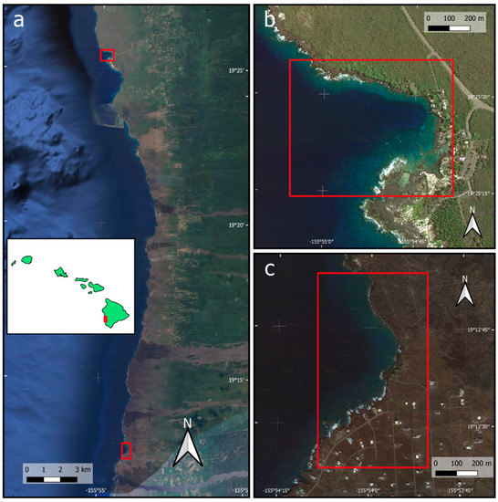
Figure 1.
(a) Location of the two study bays on the west coast of Hawai’i Island. The two right panels provide a more detailed view of (b) Honaunau Bay and (c) Pāpā Bay. Background satellite imagery © Google 2018.

Table 1.
Repeat Global Airborne Observatory data acquisitions over Honaunau and Pāpā Bays including dates, illumination and viewing geometries, and sea surface conditions.
Each data collection flight utilized two co-aligned instruments: The VSWIR imaging spectrometer and a dual-channel airborne LIDAR. During each data collection, flights were performed at an airspeed of 60 m s−1 and an elevation of 650 m above ground level for Honaunau Bay and 400 m for Pāpā Bay. The LIDAR was operated at a pulse frequency of 200 kHz, a scan frequency of 34 Hz, and an effective field-of-view of 34° to match the VSWIR spectrometer. While the 1064 nm laser of the LIDAR system does not penetrate the water surface, enough points from specular reflection of the water surface are recovered to produce a water surface map for use in spatial orthorectification of the VSWIR spectrometer data. Spectrometer data were collected in 427 spectral channels between 350 and 2500 nm in 5 nm increments [22]. Mapping conditions, including solar and sensor geometries as well as wind and tide levels, varied widely between and within each flight coverage (Table 1). This variation facilitated an analysis of the repeatability and stability of our bathymetric and 3D rugosity mapping approach.
2.2. Data Processing
Sea surface maps produced from the LIDAR data were used to orthorectify the VSWIR spectrometer data. Error in LIDAR point cloud vertical position was < 10 cm (root mean squared error) and was processed to digital surface maps using LAStools (Rapidlasso GmbH; Gilching, Germany). Each VSWIR spectrometer pixel was matched with a position and orientation from the post-processed trajectory derived from the onboard GPS-IMU navigation system, adjusted by known boresight and position offsets between the two instruments. Using a ray-tracing procedure onto the LIDAR-derived sea surface map, we determined the position of each spectrometer pixel, and used this to transform the spectrometer data into a UTM coordinate system. The final resolution of the spectrometer images was 65 cm for Honaunau Bay and 40 cm for Pāpā Bay.
The spectral radiance data recorded by the VSWIR spectrometer were converted to sea surface reflectance by accounting for lighting and atmospheric effects. For atmospheric correction, we used a modified version of the ATREM model with LIDAR-derived observation angles and elevation as inputs [20,26]. The orthorectified surface reflectance data were mosaicked for each timestep using the criterion of minimum view zenith angle for overlapping areas between adjacent flight lines.
2.3. Bathymetric Modeling
The US Army Corps of Engineers was commissioned to map portions of the Hawaiian Islands using a SHOALS system in 2013 [12]. Data from this campaign were acquired as 3D point locations describing the horizontal location of the laser returns with mean tide-corrected water depth at 6 m spatial resolution. We created a large training data set comprised of SHOALS depths and co-located VSWIR spectra for use in a regression model to estimate benthic surface depth from all overpasses of the VSWIR spectrometer recorded by the GAO in the Hawaiian Islands. Because of water absorption at longer wavelengths, the extracted GAO spectra were limited to the first 120 VSWIR bands, covering wavelengths from 346.6–942.5 nm. Across the recorded VSWIR coverage, this resulted in 18,623,871 training points, each with data for the 120 VSWIR spectral bands and SHOALS-derived depth. We did not correct for tides prior to fitting the model, as tide differences over such a large number of samples and over such a long time period were expected to average out during model training.
We used the TensorFlow package [27] in Python (Python Software Foundation) to train a feed-forward neural network with the 120 VSWIR spectral bands of spectral data as input, four hidden layers of 200 nodes each using a relu activation function, and a single node in the output layer using a linear activation function. A mean-squared-error loss function was selected. During training, we evaluated model performance in a 10-fold cross-validation approach. For each fold, 80% of the data were used for training, 10% for validation (used as stopping criteria), and 10% for a test set, arranged in such a way that each point was used in training eight times, as validation once, and as testing once.
In the end, we generated a prediction for each data point from a model in which that point was not used in the training set or as stopping criteria. We used the ADAM optimization algorithm [28] to fit the network coefficients to the training data, with an automatic stop determined as no improvement in the validation set loss value in 30 epochs. During the cross-validation, optimization took between 109 and 168 epochs before stopping criteria for each fold.
To assess value in model prediction afforded by the full 120-band spectra available from the VSWIR imaging spectrometer, we trained a second model using a transformation of the 120-band data to four broadband channels matching the spectral response and range of bands 2–5 (Blue, Green, Red, NIR) of the Sentinel-2B satellite (Figure 2) [29]. In this transformation, for each of the four Sentinal-2B bands considered, a weighted average of the spectrometer reflectance spectrum was computed, where the weight for each spectrometer band was the coefficient from the given spectral response curve at the wavelength nearest to the spectrometer band center. Input variables into the second model included these four computed spectral bands, as well as ratios of green: Blue, red: Blue, infrared: Blue, red: Green and infrared: Green, making nine factors in total. We used the same modelling approach as for the full spectrometer data, except the number of nodes in each layer was 30. With fewer parameters, optimization was faster, taking between 37 and 92 epochs to reach stopping criteria for each fold.
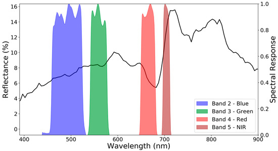
Figure 2.
Sentinel-2B spectral response curves used for calculation of the 4-band dataset derived from VSWIR imaging spectrometer data. An example Global Airborne Observatory VSWIR spectrum from 1-m deep water is given for reference. The broad bands from multi-spectral sensors average over spectral feature information.
2.4. Three-Dimensional Complexity
We applied the Vector Ruggedness Measure [30] to the bathymetric maps derived from VSWIR imaging spectroscopy and SHOALS to investigate spatial patterns derived at high spatial resolution. The VRM is a widely used surface roughness metric that incorporates variation of slope and aspect into a single measurement [31,32,33]. For each cell in a user-defined floating window, a unit vector orthogonal to the cell is decomposed using the three-dimensional location of the cell center along with the slope and aspect. The magnitude is standardized by dividing the number of cells in the neighborhood. Finally, the value is scaled with 0 representing flat and 1 as the most rugged. Typical benthic values are small (<0.4) in natural data [32]. We used two analytical window sizes to assess individual coral colony and reef-scale patterns: 7 pixels (4 m at Honaunau Bay and 3 m at Pāpā Bay) and 21 pixels (13 m at Honaunau Bay and 8 m at Pāpā Bay). To directly compare maps derived from the VSWIR and SHOALS approaches, we resampled the higher resolution VSWIR spectrometer maps using a median filter to 6 m to match the SHOALS depth maps. We then computed rugosity values for each of two grid sizes: 7 pixels (42 m) and 15 pixels (90 m). Following the comparison between VSWIR and SHOALS methods, we focused on the interpretation of the full-resolution VSWIR-based approach in order to assess reef complexity at the finest possible granularity.
3. Results
The neural network model trained with the 120-band spectra performed notably better than the model trained with the simulated 4-band data (Figure 3). The full model resulted in a root mean squared error (RMSE) between VSWIR and SHOALS of 2.0 m, with a mean absolute deviation (MAD) of 1.2 m (Figure 3b) across the aggregated test data set. The computed R2 statistic was 0.96. The model also correctly labeled 95.3% of non-water samples. Remaining non-water pixels could be filtered using additional spectral filters, where reflectance in the near- to shortwave-infrared wavelengths are near to zero over water. In comparison, the reduced 4-band model had approximately double the error, with an RMSE of 4.0 m, MAD of 2.6, and R2 of 0.82. Improvement in prediction accuracy and precision from the spectral detail available in the spectrometer data was found at all SHOALS-measured depths, reducing the errors seen in the reduced model even into the >30m water depth range. Errors can be found from both models that are attributed to a number of causes beyond model-driven error, including positional error, refraction, smoothing inherent in the 5 m SHOALS data, tide variability, waves, and data quality (e.g., shadow, glint). In both cases, model prediction error increased with depth, as the signal-to-noise ratio decreases with depth, and many of the sources of errors compound with increasing depth.
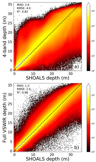
Figure 3.
Heat map scatterplots of the bathymetric values estimated from a neural network model applied to (a) simulated 4-band multispectral imagery and (b) the full VSWIR imaging spectroscopy compared to SHOALS-measured depth. Color represents point density. Isolated points of noise are typically pixels with a high amount of sea surface glint or shaded pixels, both of which can be removed from final maps.
3.1. Bathymetric Maps
The spectroscopic mapping approach provided consistent depth results among all mapping dates, which incorporated a wide range of illumination and sea conditions (Table 1; Figure 4). The repeatability of an optically-based approach proved sufficient to consider it stable for more general use. Although the VSWIR-vs-SHOALS transect comparisons indicated some areas of disagreement, the overall spectroscopic depth results matched the SHOALS depths to greater than 20 m in Pāpā Bay and 30 m in Honaunau Bay. Disagreement between the two approaches could be due to the difference in resolution in steeply sloping areas, uncertainties in either method related to positioning or water conditions, or changes in benthic structure between 2013 when the SHOALS data were collected and 2018–2019 when the VSWIR data were acquired. Nonetheless, scatterplots revealed the overall agreement between VSWIR and SHOALS approaches, showing no systematic bias and close adherence to the 1:1 line, and with RMSE values of 2.5–2.9 m for individual dates at Honaunau Bay and 2.3–3.3 m for individual dates at Pāpā Bay (Figure 5). When the various VSWIR bathymetric maps were combined and the median depth calculated, the RMSE was 2.4 m for Honaunau Bay and 1.7 m for Pāpā Bay.
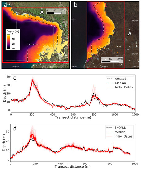
Figure 4.
Demonstration transects from (a) Honaunau Bay and (b) Pāpā Bay shown in black and white dashed lines. Green outlines show the extent of the SHOALS coverage. For the transect lines, the GAO VSWIR spectrometer-derived depth for individual dates are thin dashed red lines and the median is a thick solid red line. The SHOALS-derived depth is shown as a dashed black line for (c) Honaunau Bay and (d) Pāpā Bay. Both transects start in the south end of the given site. Background satellite imagery © Google 2018.
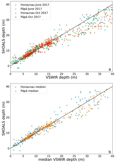
Figure 5.
Scatterplot of SHOALS-derived seafloor depth measurements against the depth estimated from VSWIR imaging spectrometer measurements. (a) Estimates by individual date. (b) Median values for all dates at each site. The solid black line is the 1:1 line.
3.2. Reef Rugosity
Comparing the native 6-m resolution SHOALS-based rugosity to a VSWIR-based rugosity map artificially coarsened to the same resolution, we found that there was general agreement between the two approaches (R2 = 0.58) (Figure 6a,b). At these coarser resolutions, rugosity mainly reveals the slope of the seafloor, and does not resolve the presence of individual coral colonies and other fine benthic features. This is a common finding in our use of data at spatial resolutions of 3 m or coarser (data not shown).
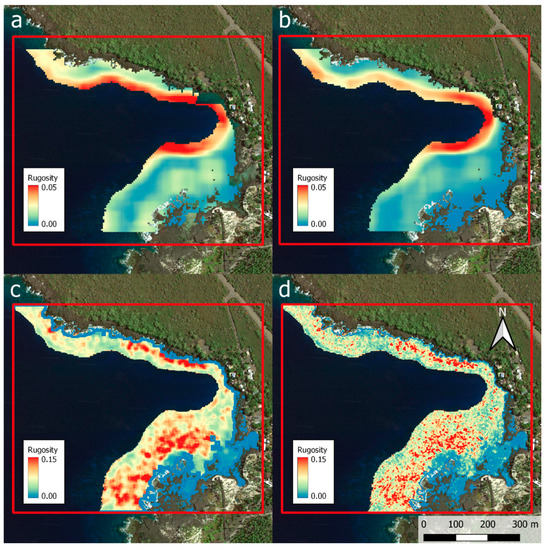
Figure 6.
Reef rugosity using a 7-pixel moving window estimated water depth from (a) SHOALS (at native 6m spatial resolution) and (b) VSWIR imaging spectroscopy (averaged to 6m spatial resolution) in Honaunau Bay to 20 m ocean depth. These course-resolution rugosity maps are essentially maps of reef slope. For comparison, the high spatial resolution provided by the VSWIR spectrometer (65 cm) affords rugosity metrics at finer resolutions, shown here with (c) 21-pixel and (d) 7-pixel moving windows, which reveal coral colonies in red areas. Background satellite imagery © Google 2018.
At finer resolutions afforded by the VSWIR mapping, the resulting rugosity maps revealed a much higher granularity of variation (Figure 6c,d). In this example from Honaunau Bay, areas of high rugosity shown in red are large individual mound- or dome-forming coral colonies or groups of coral colonies in the genera Porites and Pavona on a background of gently sloping seafloor. Our experience with the maps indicated that most coral colonies larger than 1 m in diameter are resolved as high-rugosity locations shown in red (Figure 6c,d). Notice that these coral colonies are roughly anti-correlated with seafloor slope as revealed in the SHOALS-based rugosity data (Figure 6a).
In the two research bays, median values of rugosity increased by about five times from shallow to deeper waters (Figure 7). Variation in rugosity also increased with depth. However, neither minimum nor maximum rugosity changed significantly with depth, owing to the fact that flat sand patches and isolated areas of heightened 3D complexity, such as groups of coral colonies and rock outcrops, occur at all depths. Despite these extreme values of rugosity being similar across depth ranges, the distributions of 3D complexity broadened and decreased in skewness with depth in both bays. The deepest areas of 20–25 m harbored near-normally distributed rugosities, whereas the shallower depths were more skewed to low-rugosity values.
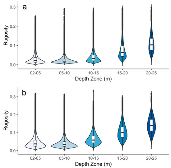
Figure 7.
Violin plots of reef rugosity versus depth (m) for (a) Pāpā Bay and (b) Honaunau Bay showing a general increase in rugosity with depth, matching observations of more complex coral habitat in deeper waters. Each plot shows the frequency distribution of high-resolution rugosity values using 40 cm and 65 cm spatial resolution bathymetry maps for Pāpā and Honaunau Bays, respectively. Box plots within violin plots indicate the median, first quartile and third quartile of the distributions.
4. Discussion
We developed and successfully tested an approach for high spatial resolution mapping of nearshore bathymetry and reef complexity in two study embayments of Hawai’i island. Our bathymetric mapping results from high-fidelity imaging spectroscopy proved highly comparable to those derived from the benchmark SHOALS laser-based methodology. We showed that the use of spectroscopic data increased both the precision and accuracy of depth estimates over what can be obtained with broad multispectral bands often used for water depth estimation. This is especially important in water deeper than 10 m, where the red band provides only noise. Similar results have been found for a hyperspectral satellite data [34]. Any successful models derived from a small number of bands is likely to be highly site-dependent, tuned to local water properties, particularly chlorophyll and dissolved solids, as well as bottom color and albedo. A large number of degrees of freedom are needed to separate these confounding variables from water depth. While attempts have been made to make models more general [18], these limitations of multispectral imagery have prevented progress in this area.
Our approach affords us the advantage to estimate water depths at spatial resolutions of much less than 1 m. Critically, we demonstrated the relative stability and repeatability of the approach among a wide range of ocean conditions (Table 1). Some constraints limit the horizontal resolution and minimum detectable object size in laser-based systems, such as a high beam divergence needed to maintain eye safety and the difficulty of engineering a green laser with high power and short pulse width capability [35]. Regardless of sensor, working at finer resolution does come with challenges, as water surface features increasingly interfere with mapping. Surface waves affect predicted depth, both because of changes in actual water depth as well as increased refraction that changes path length from the ocean floor to water surface. Additionally, surface wind can cause small waves that both produce glint, or sunlight directly reflected back into the sensor from the water surface, and whitecaps. These issues can be mitigated by blending multiple flight passes over a given area. Glint is detectable using information in bands readily absorbed by water (typically near-infrared), meaning any reflectance in these bands is glint or noise.
Despite these challenges, the high-resolution approach is advantageous because it supports the ability to map 3D reef complexity at granularities approaching that of individual coral colonies. The imaging spectroscopy-based method thus provides both benthic topographic and biological information. Using our highest spatial resolution VSWIR measurements, our reef rugosity results indicated increasing 3D complexity with depth to 25 m. These results are in general agreement with our knowledge of both study bays, and can be qualitatively linked to an increase in live coral with depth. Wave action, combined with a major bleaching event in 2015, are known drivers of decreased 3D complexity in the 2–10 m range [36]. This was particularly apparent in the high-resolution rugosity results, such as in Figure 6 for Honaunau Bay, where nearshore reefs had low rugosity values (blue tones in Figure 6). We found similar results in Pāpā Bay (data not shown).
At depths exceeding 15 m, reef complexity increases with protection from both surface waves and recent thermal events. We also note that these results are not possible with the coarser SHOALS approach, where the resolution is sufficient to resolve benthic topography but not biological structural complexity (Figure 6a). Monitoring changes in reef 3D complexity at high spatial resolution and over time will provide a means to assess the impacts of climate change and coastal processes that affect reef complexity. The cascading effects of these changes on fish, invertebrate, and other reef inhabitants will then be trackable through time.
Scaling up bathymetric and 3D reef complexity assessments from high-fidelity imaging spectroscopy will require additional airborne mapping since such instruments are not yet available from Earth orbit. Several spaceborne imaging spectrometer missions are planned or are in design phases now. For example, the NASA Surface Biology and Geology Mission (formerly HyspIRI) may be operated from low-Earth orbit in the mid-to-late 2020s [37]. However, this mission will provide high-fidelity spectroscopy at 30–45 m spatial resolution, which will preclude its use in applications at the resolutions of individual coral colonies. Several high spatial-resolution instruments (10–30 m resolution) are planned for deployments in Earth orbit, and that will be a major step toward large coral colony-scale benthic mapping. Despite these likely advances, a need for very high-resolution airborne approaches will certainly increase as reefs continue to undergo enormous yet largely unmeasured change in the coming years.
5. Conclusions
We developed a new approach for high spatial resolution (<1 m) mapping of nearshore bathymetry and three-dimensional habitat complexity (rugosity) using airborne high-fidelity imaging spectroscopy. We applied the method to two research bays on the Island of Hawai’i to ocean depths exceeding 25 m, and compared the results to the benchmark standard using laser-based SHOALS bathymetry. We showed that the increased detail afforded by imaging spectroscopy allows increased precision and accuracy over multispectral approaches. Our results proved consistent on repeat flights that incorporated a wide range of viewing and solar geometries and sea state conditions. We found that the spectroscopy-based results were comparable to those derived from SHOALS, but the former provides much higher spatial resolution depth and rugosity data. The spectroscopy-based approach thus affords mapping, monitoring, and analysis of coral colony scale changes in benthic composition.
Author Contributions
Conceptualization, G.P.A. and N.R.V.; methodology, G.P.A., N.R.V., C.B., P.G.B., and J.H.; formal analysis, N.R.V. and C.B.; writing—Original draft preparation, G.P.A. and N.R.V.; writing—Review and editing, G.P.A., N.R.V., C.B., P.G.B., and J.H.; funding acquisition, G.P.A. All authors have read and agreed to the published version of the manuscript.
Funding
This research was funded by Lenfest Ocean Program, grant number 00032718. The Global Airborne Observatory is made possible by grants and gifts from private foundations, visionary individuals, and Arizona State University.
Acknowledgments
We thank the Global Airborne Observatory team for data collection and processing support.
Conflicts of Interest
The authors declare no conflict of interest.
References
- Hoegh-Guldberg, O. Climate change, coral bleaching and the future of the world’s coral reefs. Mar. Freshw. Res. 1999, 50, 839–866. [Google Scholar] [CrossRef]
- Brown, B.E. Coral bleaching: Causes and consequences. Coral Reefs 1997, 16, S129–S138. [Google Scholar] [CrossRef]
- Carlson, R.R.; Foo, S.A.; Asner, G.P. Land use impacts on coral reef health: A ridge-to-reef perspective. Front. Mar. Sci. 2019, 6, 562. [Google Scholar] [CrossRef]
- Graham, N.A.; Jennings, S.; MacNeil, M.A.; Mouillot, D.; Wilson, S.K. Predicting climate-driven regime shifts versus rebound potential in coral reefs. Nature 2015, 518, 94–97. [Google Scholar] [CrossRef] [PubMed]
- Dustan, P.; Doherty, O.; Pardede, S. Digital reef rugosity estimates coral reef habitat complexity. PLoS ONE 2013, 8, e57386. [Google Scholar] [CrossRef] [PubMed]
- Graham, N.; Nash, K. The importance of structural complexity in coral reef ecosystems. Coral Reefs 2013, 32, 315–326. [Google Scholar] [CrossRef]
- Kuffner, I.B.; Brock, J.C.; Grober-Dunsmore, R.; Bonito, V.E.; Hickey, T.D.; Wright, C.W. Relationships between reef fish communities and remotely sensed rugosity measurements in Biscayne National Park, Florida, USA. Environ. Biol. Fishes 2007, 78, 71–82. [Google Scholar] [CrossRef]
- Harborne, A.R.; Mumby, P.J.; Ferrari, R. The effectiveness of different meso-scale rugosity metrics for predicting intra-habitat variation in coral-reef fish assemblages. Environ. Biol. Fishes 2012, 94, 431–442. [Google Scholar] [CrossRef]
- Brock, J.C.; Wright, C.W.; Clayton, T.D.; Nayegandhi, A. LIDAR optical rugosity of coral reefs in Biscayne National Park, Florida. Coral Reefs 2004, 23, 48–59. [Google Scholar] [CrossRef]
- Prada, M.; Appeldoorn, R.; Rivera, J.A. Improving coral reef habitat mapping of the Puerto Rico insular shelf using side scan sonar. Mar. Geod. 2008, 31, 49–73. [Google Scholar] [CrossRef]
- Putney, A.; Chang, E.; Chatham, R.; Marx, D.; Nelson, M.; Warman, L.K. Synthetic aperture sonar-the modern method of underwater remote sensing. In Proceedings of the 2001 IEEE Aerospace Conference Proceedings (Cat. No. 01TH8542), Big Sky, MT, USA, 10–17 March 2001; Volume 1744, pp. 4/1749–4/1756. [Google Scholar]
- Irish, J.L.; Lillycrop, W.J. Scanning laser mapping of the coastal zone: The SHOALS system. ISPRS J. Photogramm. Remote Sens. 1999, 54, 123–129. [Google Scholar] [CrossRef]
- Guenther, G.C.; Brooks, M.W.; LaRocque, P.E. New capabilities of the “SHOALS” airborne lidar bathymeter. Remote Sens. Environ. 2000, 73, 247–255. [Google Scholar] [CrossRef]
- Polcyn, F.C.; Rollin, R. Remote Sensing Techniques for the Location and Measurement of Shallow-Water Features; The University of Michigan: Ann Arbor, MI, USA, 1969. [Google Scholar]
- Eakin, C.M.; Nim, C.J.; Brainard, R.E.; Aubrecht, C.; Elvidge, C.; Gledhill, D.K.; Muller-Karger, F.; Mumby, P.J.; Skirving, W.J.; Strong, A.E. Monitoring coral reefs from space. Oceanography 2010, 23, 118–133. [Google Scholar] [CrossRef]
- Bierwirth, P.; Lee, T.; Burne, R. Shallow sea-floor reflectance and water depth derived by unmixing multispectral imagery. Photogramm. Eng. Remote Sens. 1993, 59, 331–338. [Google Scholar]
- Li, J.; Knapp, D.E.; Schill, S.R.; Roelfsema, C.; Phinn, S.; Silman, M.; Mascaro, J.; Asner, G.P. Adaptive bathymetry estimation for shallow coastal waters using Planet Dove satellites. Remote Sens. Environ. 2019, 232, 111302. [Google Scholar] [CrossRef]
- Stumpf, R.P.; Holderied, K.; Sinclair, M. Determination of water depth with high-resolution satellite imagery over variable bottom types. Limnol. Oceanogr. 2003, 48, 547–556. [Google Scholar] [CrossRef]
- Foo, S.A.; Asner, G.P. Scaling up coral reef restoration using remote sensing technology. Front. Mar. Sci. 2019, 6, 79. [Google Scholar] [CrossRef]
- Thompson, D.R.; Hochberg, E.J.; Asner, G.P.; Green, R.O.; Knapp, D.E.; Gao, B.-C.; Garcia, R.; Gierach, M.; Lee, Z.; Maritorena, S. Airborne mapping of benthic reflectance spectra with Bayesian linear mixtures. Remote Sens. Environ. 2017, 200, 18–30. [Google Scholar] [CrossRef]
- Lesser, M.; Mobley, C. Bathymetry, water optical properties, and benthic classification of coral reefs using hyperspectral remote sensing imagery. Coral Reefs 2007, 26, 819–829. [Google Scholar] [CrossRef]
- Asner, G.P.; Knapp, D.E.; Boardman, J.; Green, R.O.; Kennedy-Bowdoin, T.; Eastwood, M.; Martin, R.E.; Anderson, C.; Field, C.B. Carnegie Airborne Observatory-2: Increasing science data dimensionality via high-fidelity multi-sensor fusion. Remote Sens. Environ. 2012, 124, 454–465. [Google Scholar] [CrossRef]
- Chapman, J.W.; Thompson, D.R.; Helmlinger, M.C.; Bue, B.D.; Green, R.O.; Eastwood, M.L.; Geier, S.; Olson-Duvall, W.; Lundeen, S.R. Spectral and radiometric calibration of the next generation airborne visible infrared spectrometer (AVIRIS-NG). Remote Sens. 2019, 11, 2129. [Google Scholar] [CrossRef]
- Mouroulis, P.; Green, R.O.; Chrien, T.G. Design of pushbroom imaging spectrometers for optimum recovery of spectroscopic and spatial information. Appl. Opt. 2000, 39, 2210–2220. [Google Scholar] [CrossRef] [PubMed]
- Kramer, K.; Cotton, S.; Lamson, M.; Walsh, W. Bleaching and catastrophic mortality of reef-building corals along west Hawai’i island: Findings and future directions. In Proceedings of the 13th International Coral Reef Symposium, Honolulu, Hawaii, 19–24 June 2016. [Google Scholar]
- Gao, B.-C.; Goetz, A.F.H. Column atmospheric water vapor and vegetation liquid water retrievals from airborne imaging spectrometer data. J. Geophys. Res. 1990, 95, 3549–3564. [Google Scholar] [CrossRef]
- Abadi, M.; Agarwal, A.; Barham, P.; Brevdo, E.; Chen, Z.; Citro, C.; Corrado, G.S.; Davis, A.; Dean, J.; Devin, M. TensorFlow: Large-scale machine learning on heterogeneous distributed systems. arXiv 2016, arXiv:1603.04467. [Google Scholar]
- Kingma, D.; Ba, J. Adam: A method for stochastic optimization. arXiv 2014, arXiv:1412.6980. [Google Scholar]
- Drusch, M.; Del Bello, U.; Carlier, S.; Colin, O.; Fernandez, V.; Gascon, F.; Hoersch, B.; Isola, C.; Laberinti, P.; Martimort, P.; et al. Sentinel-2: ESA’s optical high-resolution mission for GMES operational services. Remote Sens. Environ. 2012, 120, 25–36. [Google Scholar] [CrossRef]
- Sappington, J.M.; Longshore, K.M.; Thompson, D.R. Quantifying landscape ruggedness for animal habitat analysis: A case study using bighorn sheep in the Mojave Desert. Wildfire 2007, 71, 1419–1427. [Google Scholar] [CrossRef]
- Magel, J.M.T.; Burns, J.H.R.; Gates, R.D.; Baum, J.K. Effects of bleaching-associated mass coral mortality on reef structural complexity across a gradient of local disturbance. Sci. Rep. 2019, 9, 2512. [Google Scholar] [CrossRef]
- Walbridge, S.; Slocum, N.; Pobuda, M.; Wright, D.J. Unified geomorphological analysis workflows with Benthic Terrain Modeler. Geosciences 2018, 8, 94. [Google Scholar] [CrossRef]
- Price, D.M.; Robert, K.; Callaway, A.; Lo lacono, C.; Hall, R.A.; Huvenne, V.A.I. Using 3D photogrammetry from ROV video to quantify cold-water coral reef structural complexity and investigate its influence on biodiversity and community assemblage. Coral Reefs 2019, 28, 1007–1021. [Google Scholar] [CrossRef]
- Lee, Z.; Weidemann, A.; Arnone, R. Combined effect of reduced band number and increased bandwidth on shallow water remote sensing: The case of WorldView 2. IEEE Trans. Geosci. Remote Sens. 2013, 51, 2577–2586. [Google Scholar] [CrossRef]
- Guenther, G.C. Airborne lidar bathymetry. Digit. Elev. Model Technol. Appl. DEM Users Man. 2007, 2, 253–320. [Google Scholar]
- Rodgers, K.S.; Bahr, K.D.; Jokiel, P.L.; Donà, A.R. Patterns of bleaching and mortality following widespread warming events in 2014 and 2015 at the Hanauma Bay Nature Preserve, Hawai’i. PeerJ 2017, 5, e3355. [Google Scholar] [CrossRef] [PubMed]
- Lee, C.M.; Cable, M.L.; Hook, S.J.; Green, R.O.; Ustin, S.L.; Mandl, D.J.; Middleton, E.M. An introduction to the NASA Hyperspectral InfraRed Imager (HyspIRI) mission and preparatory activities. Remote Sens. Environ. 2015, 167, 6–19. [Google Scholar] [CrossRef]


© 2020 by the authors. Licensee MDPI, Basel, Switzerland. This article is an open access article distributed under the terms and conditions of the Creative Commons Attribution (CC BY) license (http://creativecommons.org/licenses/by/4.0/).