A Robust Deep Learning Approach for Spatiotemporal Estimation of Satellite AOD and PM2.5


Abstract

1. Introduction
2. Materials
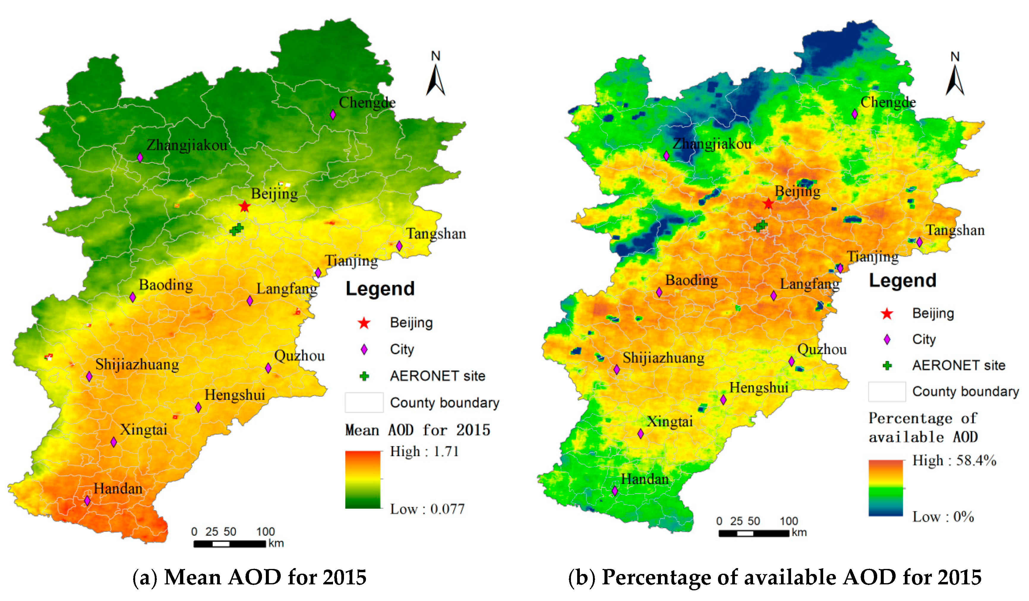
2.1. Study Region
2.2. Measurement Data
2.2.1. Satellite-Derived AOD
2.2.2. AERONET AOD
2.2.3. Ground Truth PM2.5 Measurements
2.3. Data of the Covariates
2.4. MAIAC AOD for Estimation of Daily PM2.5
3. Methods
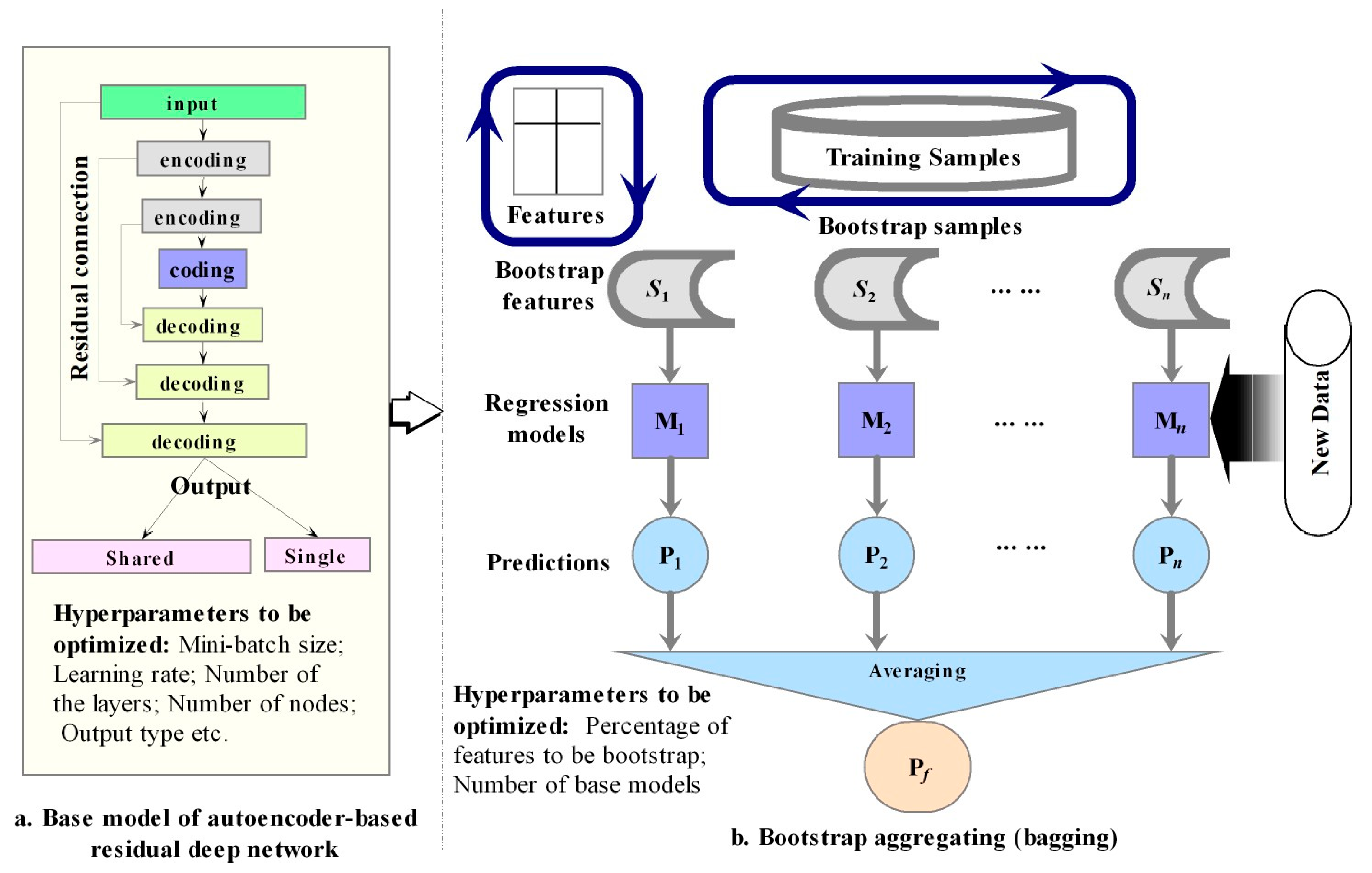
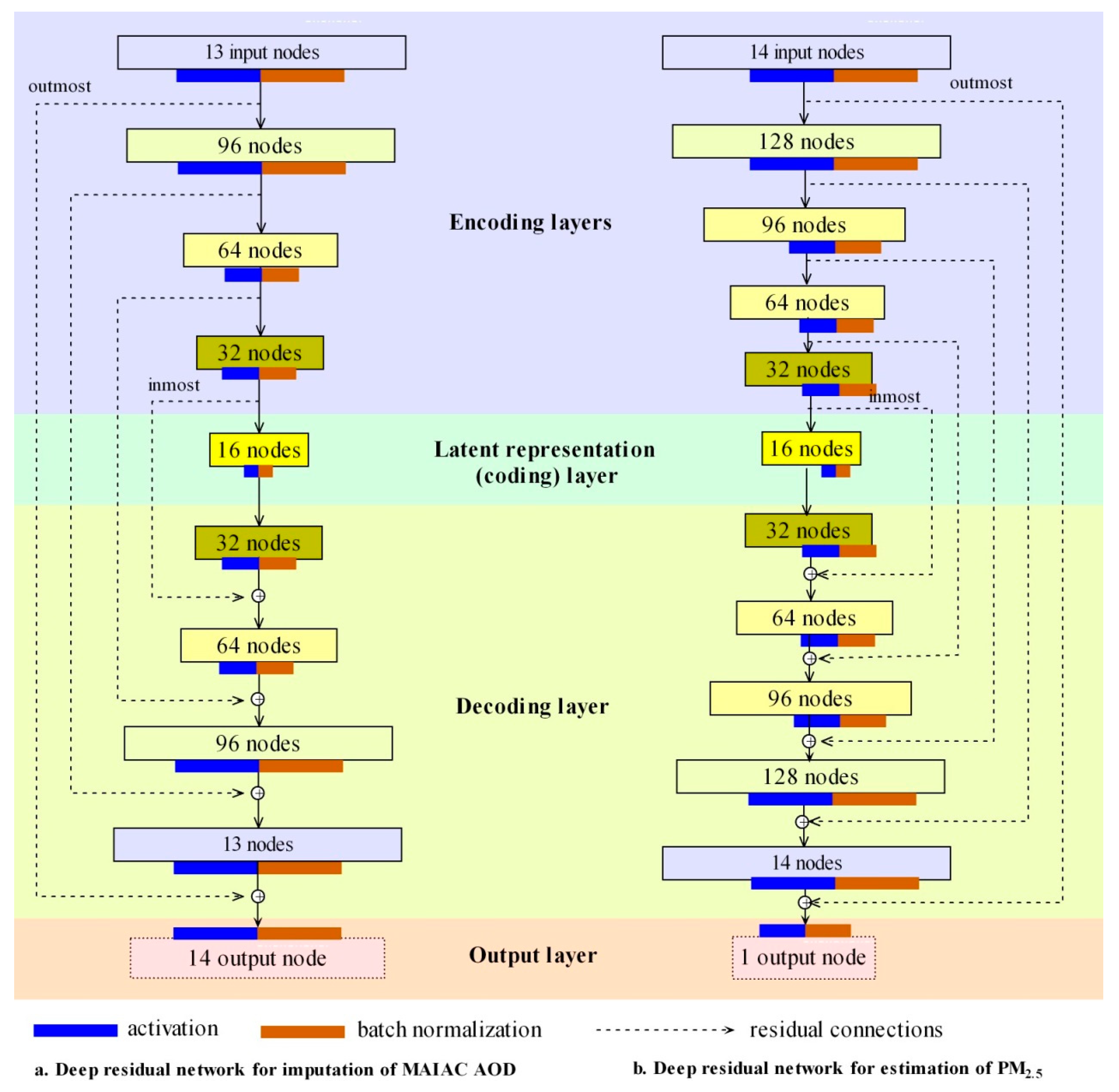
3.1. Autoencoder-based Residual Network
3.2. Bagging of Residual Networks
3.3. Model Training
3.4. Validation and Independent Test
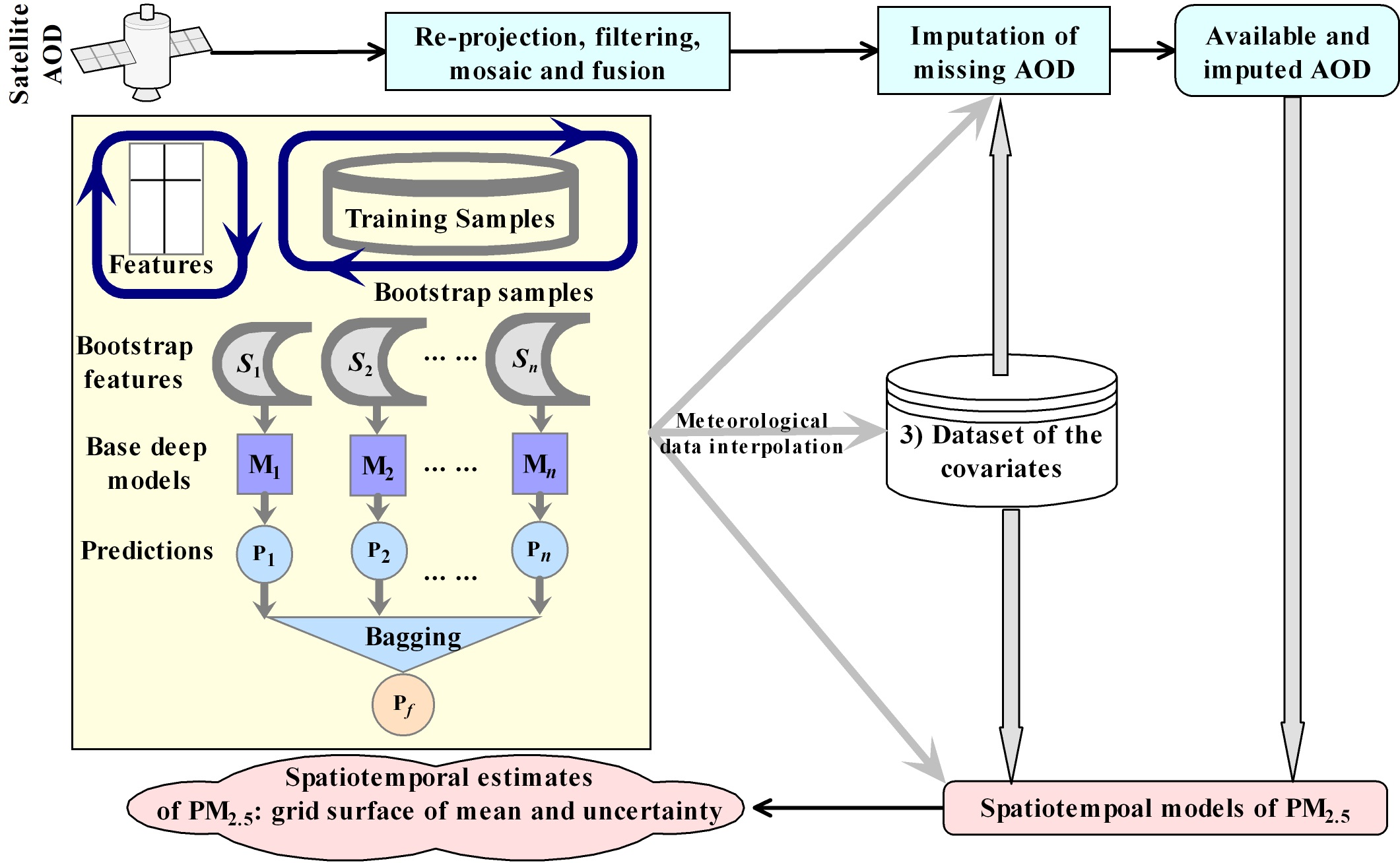
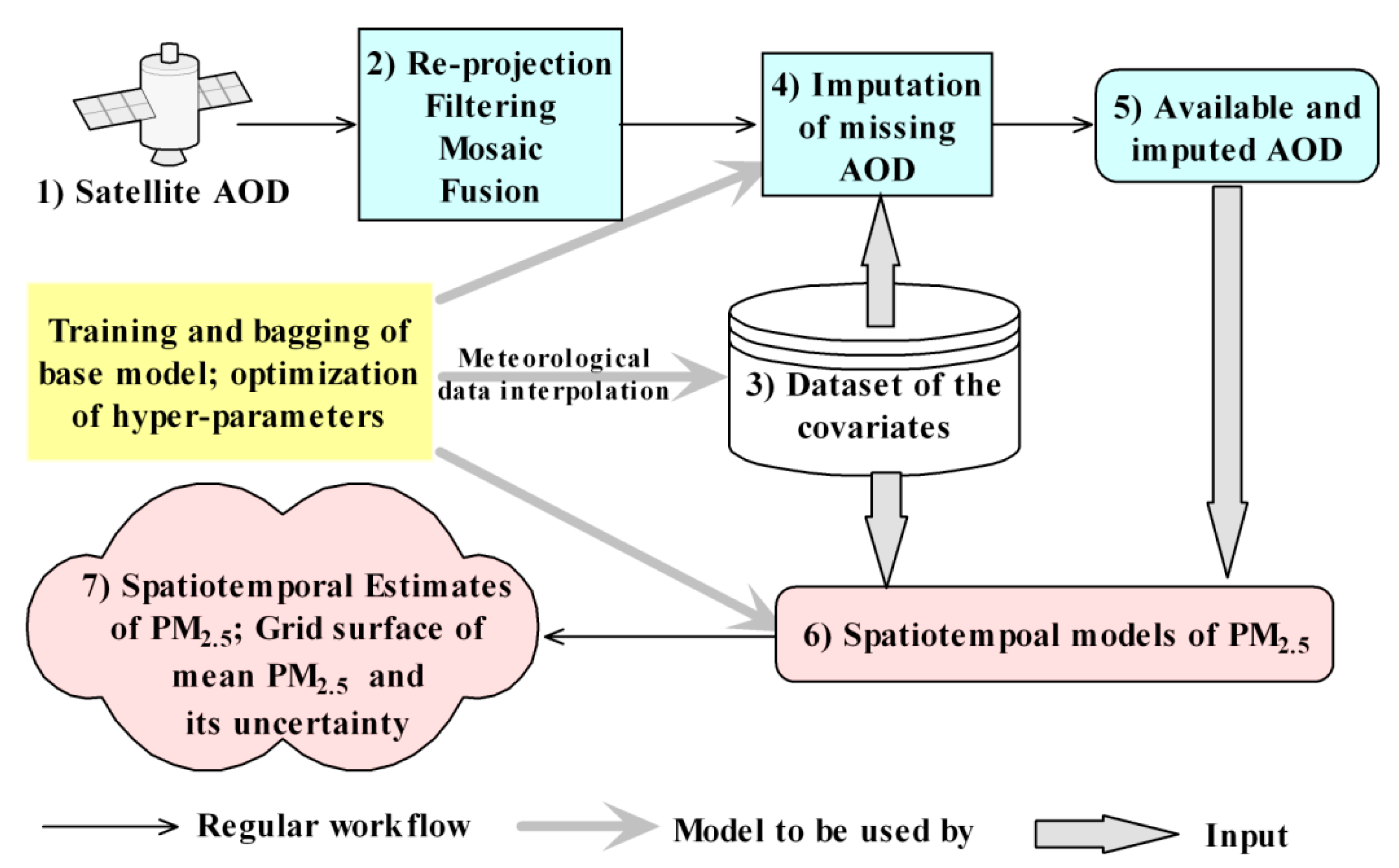
3.5. Workflow for Imputation of MAIAC AOD and Estimtion of PM2.5
- (1)
- Collection of satellite AOD data (i.e., MAIAC AOD for this study). This involved matching of the image tiles in time and space with the study region, and data downloading.
- (2)
- Pre-processing of satellite data. This involved re-projection of the satellite images to the target coordinate system, filtering of invalid and noisy AOD, possible mosaic, cropping and masking of image tiles for the study region, and fusion of images from different sources (i.e., Aqua and Terra sensors, see Supplementary Section S1 for details).
- (3)
- Collection and pre-processing of the covariates. The covariates included meteorological factors, MERRA2 data (e.g., PBLH and coarse-resolution AOD), coordinates, and elevation etc. Pre-processing involved the removal of noisy data, re-projection and re-sampling of the data from different sources, and the fusion of meteorological data. The method of the residual deep network was used for the interpolation of meteorological data. For details, please refer to Supplementary Section S2 and [85,86].
- (4)
- Imputation of missing satellite AOD. The core method proposed was used for imputation. This step involved training, validation, and testing of the daily-level imputation models (Figure 2a), and bagging (Figure 3) of multiple outputs. A grid search was conducted to retrieve optimal hyper-parameters for imputation.
- (5)
- The fusion of available and imputed satellite AOD. This involved the mosaic of both AOD, validation of the results, and check of the output to ensure the justification (e.g., a reasonable transition between available and imputed AOD).
- (6)
- Estimation of spatiotemporal PM2.5. The covariates dataset from (3) and the satellite AOD with the complete spatiotemporal coverage from (5) were used as the input of explanatory variables. Optimization of the base models (Figure 2b) and bagging was conducted by grid search in training, validation, and testing. Ensemble averaging over the outputs from multiple models was made to get the final mean and standard deviation of PM2.5.
- (7)
- Grid output of ensemble predictions and standard deviation (as an uncertainty indicator) of PM2.5 at high spatiotemporal resolution.
4. Results
4.1. Data Summary
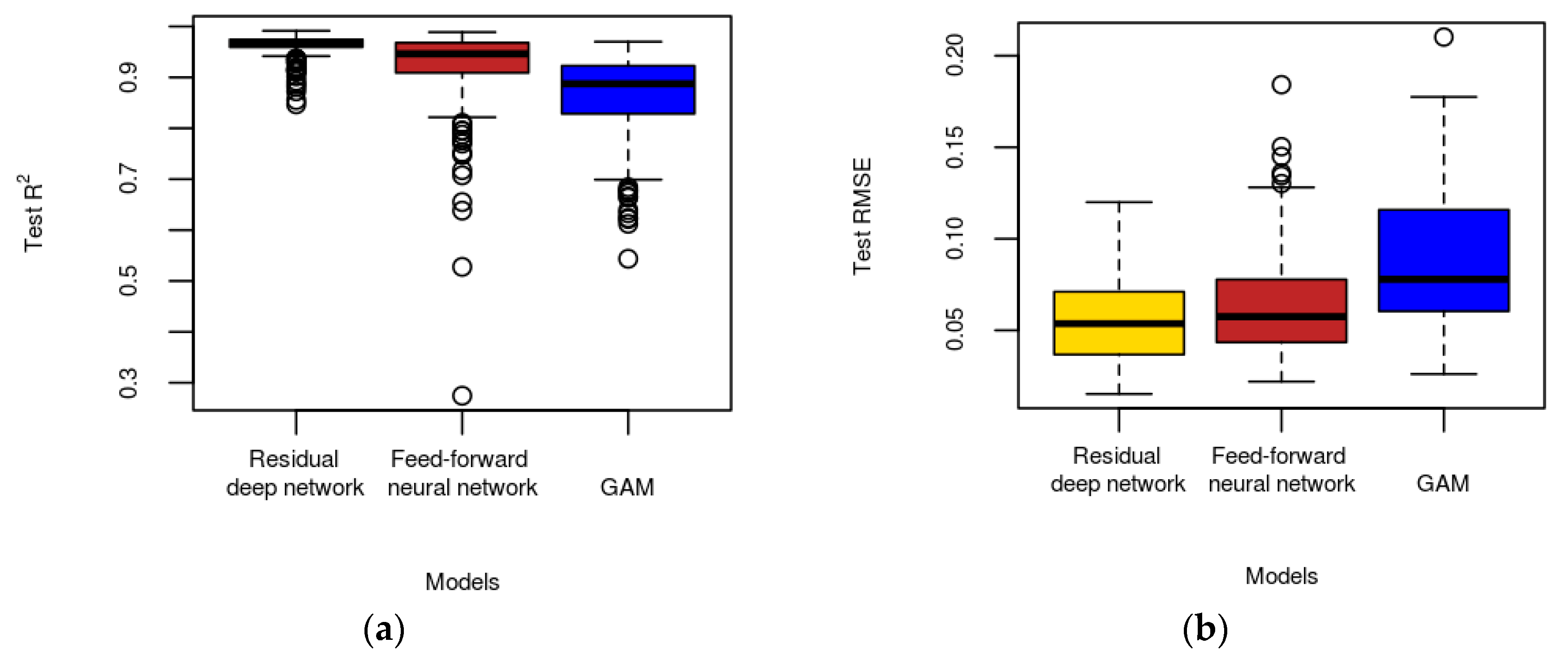
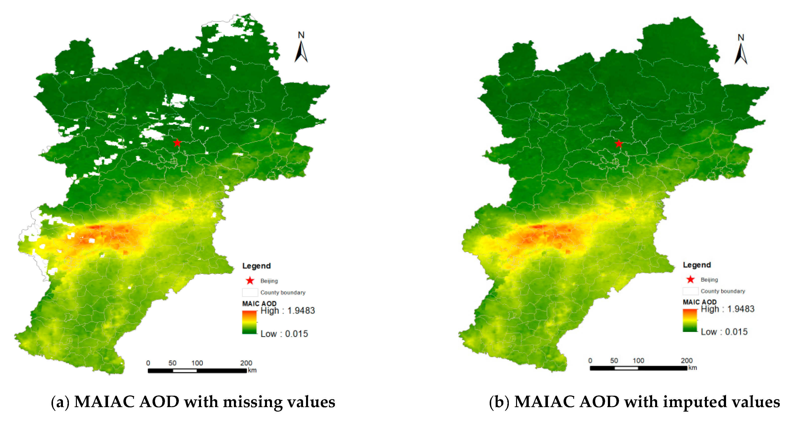
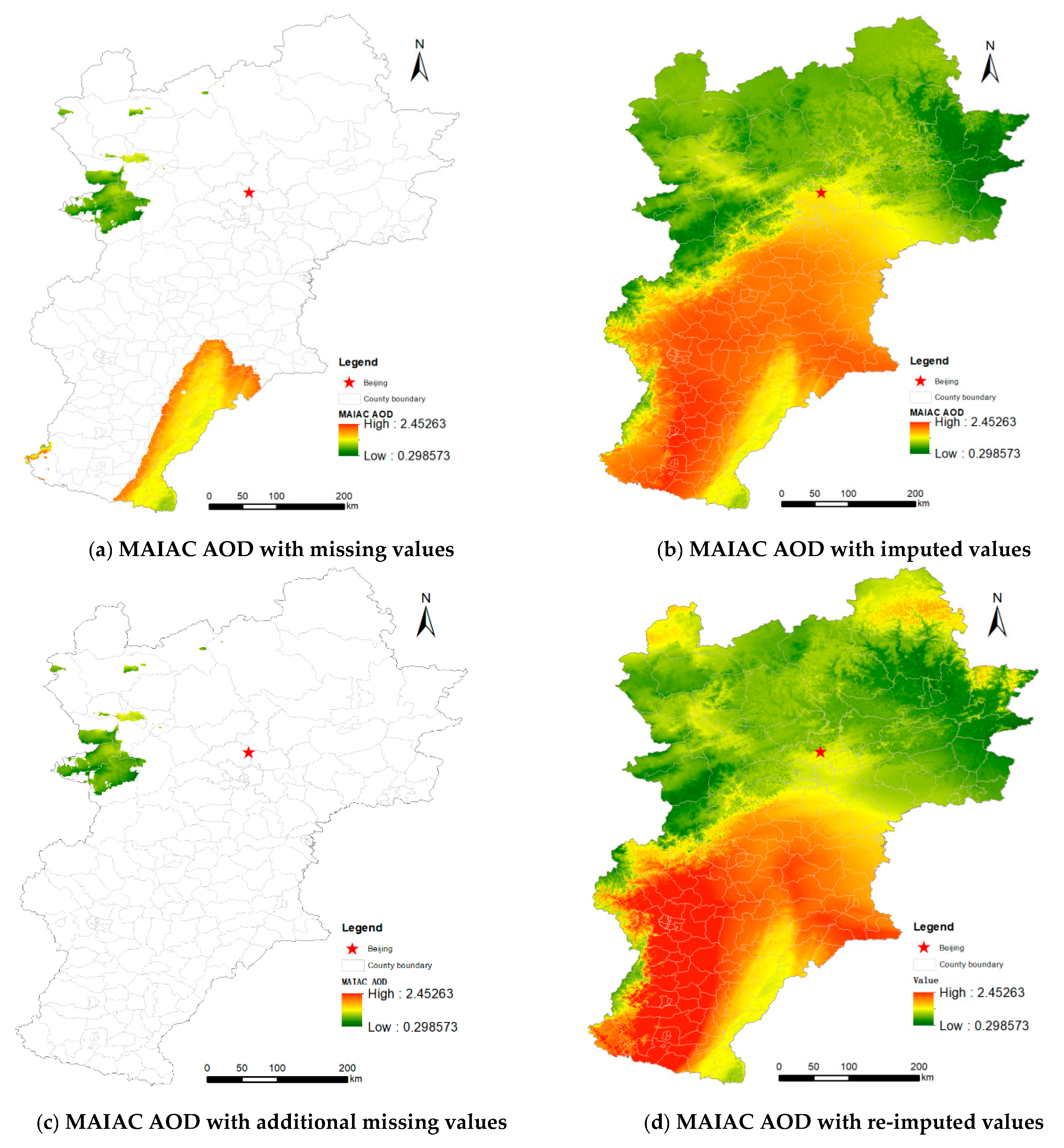
4.2. Daily-Level Imputation of MAIAC AOD
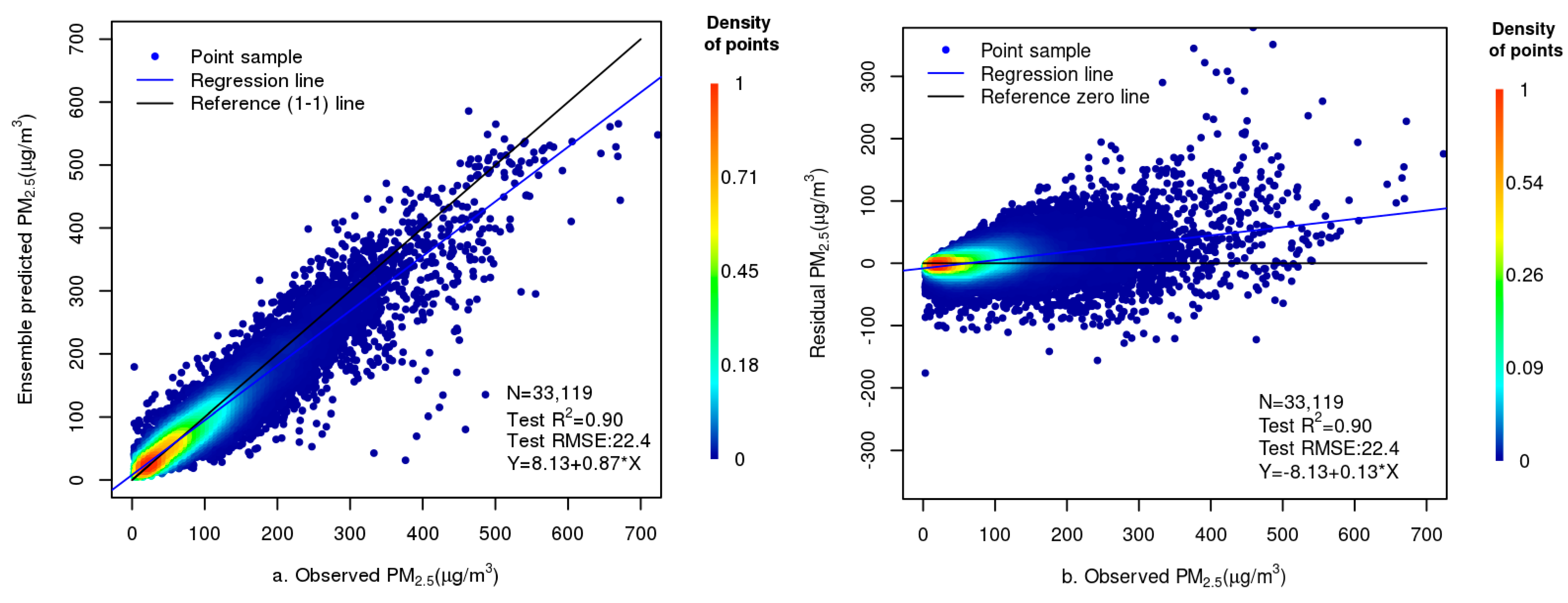
4.3. Spatiotemporal Estimation of PM2.5
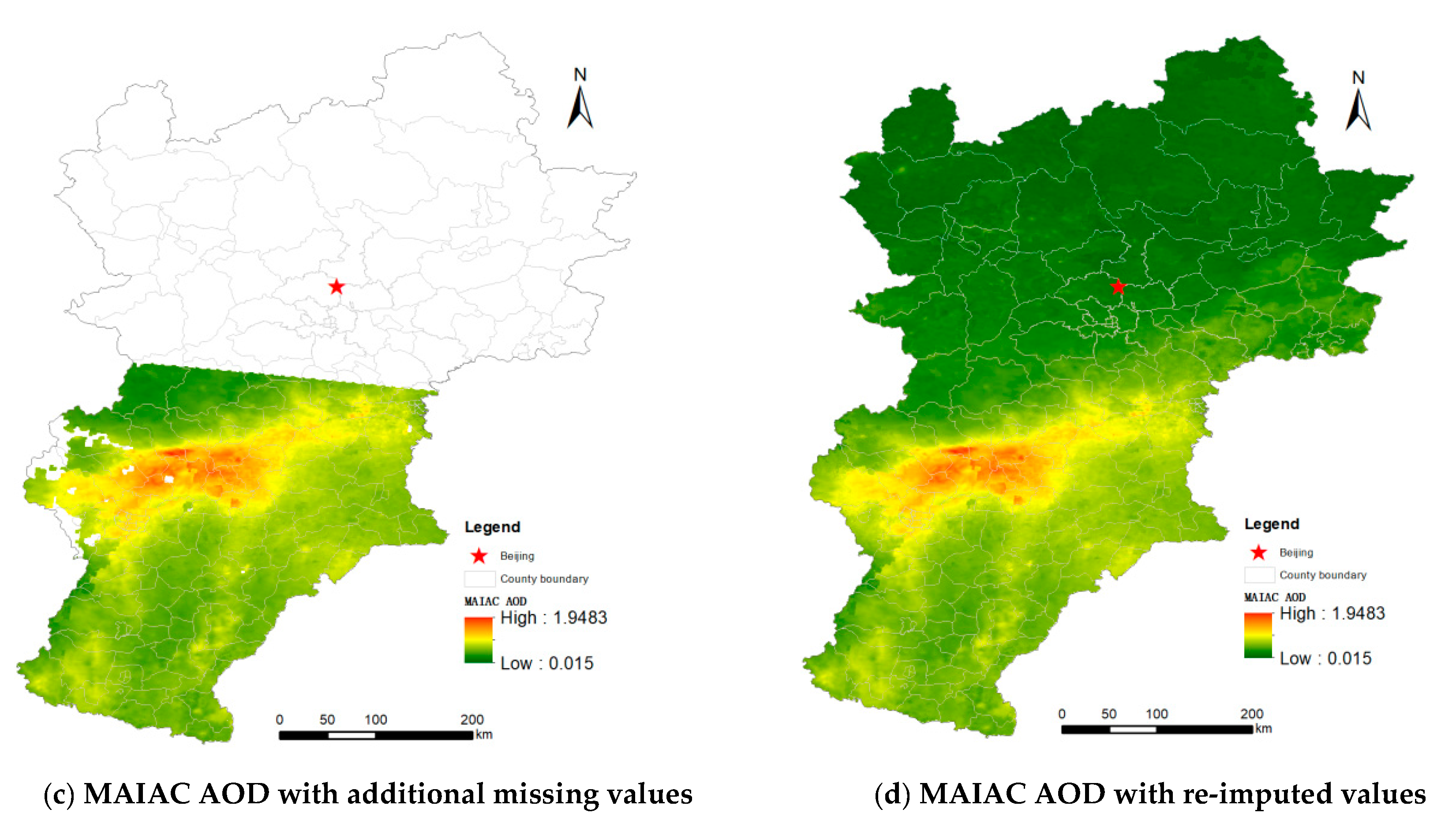
4.4. Additional Independent Test
5. Discussion
5.1. Strengths of Bagging of Residual Networks
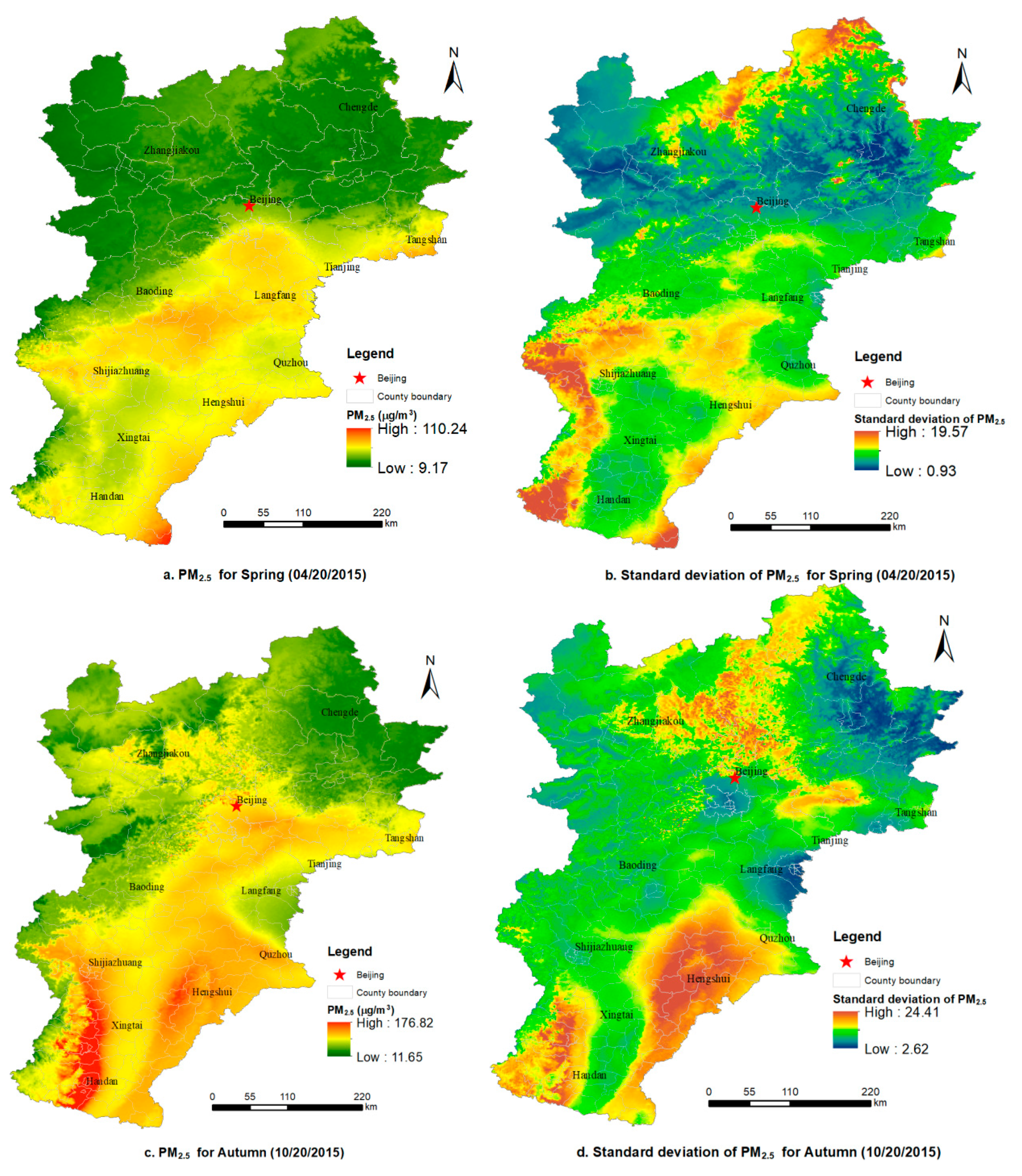
5.2. Spatiotemporal Variability of Predicted PM2.5
5.3. Uncertainty in Predicted PM2.5
5.4. Limitation and Prospects
6. Conclusions
Supplementary Materials
Author Contributions
Funding
Acknowledgments
Conflicts of Interest
References
- EPA. Health and Environmental Effects of Particulate Matter (PM). Available online: https://www.epa.gov/pm-pollution/health-and-environmental-effects-particulate-matter-pm (accessed on 1 September 2019).
- WHO. Health Effects of Particular Matter: Policy Implications for Countries in Eastern Europe, Caucasus and Central ASIA; The WHO Regional Office for Europe: Copenhagen, Denmark, 2013. [Google Scholar]
- WHO. Review of Evidence on Health Aspects of Air Pollution—REVIHAAP Project: Final Technical Report; The WHO European Centre for Environment and Health: Bonn, Switzerland, 2013. [Google Scholar]
- Kato, Y. Application of dust and PM2.5 detection methods using MODIS data to the Asian dust events which aggravated Respiratory Symptoms in Western Japan in May 2011. Proc. SPIE 2018, 10776. [Google Scholar] [CrossRef]
- Prieto-Parra, L.; Yohannessen, K.; Brea, C.; Vidal, D.; Ubilla, C.A.; Ruiz-Rudolph, P. Air pollution, PM2.5 composition, source factors, and respiratory symptoms in asthmatic and nonasthmatic children in Santiago, Chile. Environ. Int. 2017, 101, 190–200. [Google Scholar] [CrossRef]
- Zeng, X.; Xu, X.J.; Zheng, X.B.; Reponen, T.; Chen, A.M.; Huo, X. Heavy metals in PM2.5 and in blood, and children’s respiratory symptoms and asthma from an e-waste recycling area. Environ. Pollut. 2016, 210, 346–353. [Google Scholar] [CrossRef]
- Jung, K.H.; Torrone, D.; Lovinsky-Desir, S.; Perzanowski, M.; Bautista, J.; Jezioro, J.R.; Hoepner, L.; Ross, J.; Perera, F.P.; Chillrud, S.N.; et al. Short-term exposure to PM2.5 and vanadium and changes in asthma gene DNA methylation and lung function decrements among urban children. Resp. Res. 2017, 18. [Google Scholar] [CrossRef]
- Williams, A.M.; Phaneuf, D.J.; Barrett, M.A.; Su, J.G. Short-term impact of PM2.5 on contemporaneous asthma medication use: Behavior and the value of pollution reductions. Proc. Natl. Acad. Sci. USA 2019, 116, 5246–5253. [Google Scholar] [CrossRef] [PubMed]
- Dabass, A.; Talbott, E.O.; Rager, J.R.; Marsh, G.M.; Venkat, A.; Holguin, F.; Sharma, R.K. Systemic inflammatory markers associated with cardiovascular disease and acute and chronic exposure to fine particulate matter air pollution (PM2.5) among US NHANES adults with metabolic syndrome. Environ. Res. 2018, 161, 485–491. [Google Scholar] [CrossRef] [PubMed]
- Vidale, S.; Campana, C. Ambient air pollution and cardiovascular diseases: From bench to bedside. Eur. J. Prev. Cardiol. 2018, 25, 818–825. [Google Scholar] [CrossRef] [PubMed]
- Thaller, E.I.; Petronella, S.A.; Hochman, D.; Howard, S.; Chhikara, R.S.; Brooks, E.G. Moderate increases in ambient PM2.5 and ozone are associated with lung function decreases in beach lifeguards. J. Occup. Environ. Med. 2008, 50, 202–211. [Google Scholar] [CrossRef]
- Apte, J.S.; Marshall, J.D.; Cohen, A.J.; Brauer, M. Addressing global mortality from ambient PM2.5. Environ. Sci. Technol. 2015, 49, 8057–8066. [Google Scholar] [CrossRef] [PubMed]
- David, M.L.; Ravishankara, R.A.; Kodros, J.; Pierce, R.J.; Venkataraman, C.; Sadavarte, P. Premature mortality due to PM2.5 over India: effect of atmospheric transport and anthropogenic emissions. GeoHealth 2018, 3, 2–10. [Google Scholar] [CrossRef]
- Wang, X.; Dickinson, R.; Su, L.; Zhou, C.; Wang, K. PM2.5 Pollution in China and how it has been exacerbated by terrain and meteorological Conditions. Bull. Am. Meteor. Soc. 2017, 99, 105–119. [Google Scholar] [CrossRef]
- BMEPB. Main Sources of PM2.5 in Beijing: Vehicles, Coal Burning, Industry, Dust and Neighboring Cities. Available online: https://cleanairasia.org/node12353/ (accessed on 1 July 2019).
- BMEPB. A New Round of Beijing PM2.5 Source Analysis Officially Released. Available online: http://www.bjepb.gov.cn/bjhrb/xxgk/jgzn/jgsz/jjgjgszjzz/xcjyc/xwfb/607219/index.html (accessed on 1 July 2019).
- Sofowote, U.; Healy, R.; Su, Y.; Debosz, J.; Noble, M.; Munoz, A.; Jeong, C.-H.; Wang, J.; Hilker, N.; Evans, G.J. Understanding the PM2.5 imbalance between a far and near-road location: Results of high temporal frequency source apportionment and parameterization of black carbon. Atmos. Environ. 2018, 173, 277–288. [Google Scholar] [CrossRef]
- Xu, M.; Sbihi, H.; Pan, X.; Brauer, M. Local variation of PM2.5 and NO2 concentrations within metropolitan Beijing. Atmos. Environ. 2019, 200, 254–263. [Google Scholar] [CrossRef]
- Zhang, X.; Craft, E.; Zhang, K. Characterizing spatial variability of air pollution from vehicle traffic around the Houston Ship Channel area. Atmos. Environ. 2017, 161, 167–175. [Google Scholar] [CrossRef]
- Sierra-Vargas, M.P.; Teran, L.M. Air pollution: Impact and prevention. Respirology 2012, 17, 1031–1038. [Google Scholar] [CrossRef]
- Cai, S.Y.; Wang, Y.J.; Zhao, B.; Wang, S.X.; Chang, X.; Hao, J.M. The impact of the “Air Pollution Prevention and Control Action Plan” on PM2.5 concentrations in Jing-Jin-Ji region during 2012–2020. Sci. Total Environ. 2017, 580, 197–209. [Google Scholar] [CrossRef]
- Yu, A.Y.; Jia, G.S.; You, J.X.; Zhang, P.W. Estimation of PM2.5 concentration efficiency and potential public mortality reduction in urban China. Int. J. Environ. Res. Public Health 2018, 15, 529. [Google Scholar] [CrossRef]
- Wong, C.M.; Lai, H.K.; Tsang, H.; Thach, T.Q.; Thomas, G.N.; Lam, K.B.H.; Chan, K.P.; Yang, L.; Lau, A.K.H.; Ayres, J.G.; et al. Satellite-based estimates of long-term exposure to fine particles and association with mortality in elderly Hong Kong residents. Environ. Health Perspect. 2015, 123, 1167–1172. [Google Scholar] [CrossRef]
- Lall, R.; Kendall, M.; Ito, K.; Thurston, D.G. Estimation of historical annual PM2.5 exposures for health effects assessment. Atmos. Environ. 2004, 38, 5217–5226. [Google Scholar] [CrossRef]
- Yu, H.; Wang, C. Retrospective prediction of intraurban spatiotemporal distribution of PM2.5 in Taipei. Atmos. Environ. 2010, 44, 3053–3065. [Google Scholar]
- Reyes, J.M.; Serre, M.L. An LUR/BME framework to estimate PM2.5 explained by on road mobile and stationary sources. Environ. Sci. Technol. 2014, 48, 1736–1744. [Google Scholar] [CrossRef] [PubMed]
- Eeftens, M.; Meier, R.; Schindler, C.; Aguilera, I.; Phuleria, H.; Ineichen, A.; Davey, M.; Ducret-Stich, R.; Keidel, D.; Probst-Hensch, N.; et al. Development of land use regression models for nitrogen dioxide, ultrafine particles, lung deposited surface area, and four other markers of particulate matter pollution in the Swiss SAPALDIA regions. Environ. Health 2016, 15. [Google Scholar] [CrossRef] [PubMed]
- Sampson, P.D.; Richards, M.; Szpiro, A.A.; Bergen, S.; Sheppard, L.; Larson, T.V.; Kaufman, J.D. A regionalized national universal kriging model using Partial Least Squares regression for estimating annual PM2.5 concentrations in epidemiology. Atmos. Environ. 2013, 75, 383–392. [Google Scholar] [CrossRef] [PubMed]
- NASA. Aerosol Optimal Depth. Available online: https://aeronet.gsfc.nasa.gov/new_web/Documents/Aerosol_Optical_Depth.pdf (accessed on 5 August 2019).
- Bey, I.; Jacob, D.J.; Yantosca, R.M.; Logan, J.A.; Field, B.D.; Fiore, A.M.; Li, Q.B.; Liu, H.G.Y.; Mickley, L.J.; Schultz, M.G. Global modeling of tropospheric chemistry with assimilated meteorology: Model description and evaluation. J. Geophys Res. Atmos. 2001, 106, 23073–23095. [Google Scholar] [CrossRef]
- Byun, D.W.; Ching, J. Science Algorithms of the EPA Models-3 Community Multiscale Air Quality (CMAQ) Modeling System; United States Environmental Protection Agency: Washington, DC, USA, 1999. [Google Scholar]
- Appel, K.W.; Chemel, C.; Roselle, S.J.; Francis, X.V.; Hu, R.M.; Sokhi, R.S.; Rao, S.T.; Galmarini, S. Examination of the Community Multiscale Air Quality (CMAQ) model performance over the North American and European domains. Atmos. Environ. 2012, 53, 142–155. [Google Scholar] [CrossRef]
- Quennehen, B.; Raut, J.C.; Law, K.S.; Daskalakis, N.; Ancellet, G.; Clerbaux, C.; Kim, S.W.; Lund, M.T.; Myhre, G.; Olivie, D.J.L.; et al. Multi-model evaluation of short-lived pollutant distributions over east Asia during summer 2008. Atmos. Chem. Phys. 2016, 16, 10765–10792. [Google Scholar] [CrossRef]
- Hsu, N.C.; Tsay, S.C.; King, M.D.; Herman, J.R. Aerosol properties over bright-reecting source regions. IEEE Trans. Geosci. Remote Sens. 2004, 42, 557–569. [Google Scholar] [CrossRef]
- Levy, R.C.; Remer, L.A.; Mattoo, S.; Vermote, E.F.; Kaufman, Y.J. Second-generation operational algorithm: retrieval of aerosol properties over land from inversion of Moderate Resolution Imaging Spectroradiometer spectral reflectance. J. Geophys. Res. Atmos. 2007, 112. [Google Scholar] [CrossRef]
- Hsu, N.; Jeong, M.J.; Bettenhausen, C.; Sayer, A.; Hansell, R.; Seftor, C.; Huang, J.; Tsay, S.C. Enhanced Deep Blue aerosol retrieval algorithm: The second generation. J. Geophys. Res. Atmos. 2013, 118, 9296–9315. [Google Scholar] [CrossRef]
- Hsu, N.C.; Tsay, S.-C.; King, M.D.; Herman, J.R. Deep blue retrievals of Asian aerosol properties during ACE-Asia. IEEE T. Geosci. Remote 2006, 44, 3180–3195. [Google Scholar] [CrossRef]
- Engel-Cox, J.A.; Holloman, C.H.; Coutant, B.W.; Hoff, R.M. Qualitative and quantitative evaluation of MODIS satellite sensor data for regional and urban scale air quality. Atmos. Environ. 2004, 38, 2495–2509. [Google Scholar] [CrossRef]
- Liu, Y.; Park, R.J.; Jacob, D.J.; Li, Q.B.; Kilaru, V.; Sarnat, J.A. Mapping annual mean ground-level PM2.5 concentrations using Multiangle Imaging Spectroradiometer aerosol optical thickness over the contiguous United States. J. Geophys. Res. Atmos. 2004, 109. [Google Scholar] [CrossRef]
- Gupta, P.; Christopher, S.A.; Wang, J.; Gehrig, R.; Lee, Y.; Kumar, N. Satellite remote sensing of particulate matter and air quality assessment over global cities. Atmos. Environ. 2006, 40, 5880–5892. [Google Scholar] [CrossRef]
- Paciorek, C.J.; Liu, Y.; Moreno-Macias, H.; Kondragunta, S. Spatiotemporal associations between GOES aerosol optical depth retrievals and ground-level PM(2.5). Environ. Sci. Technol. 2008, 42, 5800–5806. [Google Scholar] [CrossRef]
- Wang, J.; Christopher, S.A. Intercomparison between satellite-derived aerosol optical thickness and PM2.5 mass: Implications for air quality studies. Geophys. Res. Lett. 2003, 30. [Google Scholar] [CrossRef]
- Van Donkelaar, A.; Martin, R.V.; Brauer, M.; Kahn, R.; Levy, R.; Verduzco, C.; Villeneuve, P.J. Global estimates of ambient fine particulate matter concentrations from satellite-based aerosol optical depth: Development and application. Environ. Health Perspect. 2010, 118, 847–855. [Google Scholar] [CrossRef]
- Sorek-Hamer, M.; Strawa, A.W.; Chatfield, R.B.; Esswein, R.; Cohen, A.; Broday, D.M. Improved retrieval of PM2.5 from satellite data products using non-linear methods. Environ. Pollut. 2013, 182, 417–423. [Google Scholar] [CrossRef]
- Lee, H.J.; Liu, Y.; Coull, B.A.; Schwartz, J.; Koutrakis, P. A novel calibration approach of MODIS AOD data to predict PM2.5 concentrations. Atmos. Chem. Phys. 2011, 11, 7991–8002. [Google Scholar] [CrossRef]
- Xie, Y.; Wang, Y.; Zhang, K.; Dong, W.; Lv, B.; Bai, Y. Daily estimation of ground-level PM2.5 concentrations over Beijing using 3 km resolution MODIS AOD. Environ. Sci. Technol. 2015, 49, 12280–12288. [Google Scholar] [CrossRef]
- Li, T.; Shen, H.; Zeng, C.; Yuan, Q.; Zhang, L. Point-surface fusion of station measurements and satellite observations for mapping PM2.5 distribution in China: Methods and assessment. Atmos. Environ. 2017, 152, 477–489. [Google Scholar] [CrossRef]
- Zhan, Y.; Luo, Y.Z.; Deng, X.F.; Chen, H.J.; Grieneisen, M.L.; Shen, X.Y.; Zhu, L.Z.; Zhang, M.H. Spatiotemporal prediction of continuous daily PM2.5 concentrations across China using a spatially explicit machine learning algorithm. Atmos. Environ. 2017, 155, 129–139. [Google Scholar] [CrossRef]
- Guo, Y.; Tang, Q.; Gong, D.; Zhang, Z. Estimating ground-level PM2.5 concentrations in Beijing using a satellite-based geographically and temporally weighted regression model. Remote Sens. Environ. 2017, 198, 140–149. [Google Scholar] [CrossRef]
- Lyapustin, A.; Wang, Y.; Laszlo, I.; Kahn, R.; Korkin, S.; Remer, L.; Levy, R.; Reid, J.S. Multiangle implementation of atmospheric correction (MAIAC): 2. Aerosol algorithm. J. Geophys. Res. Atmos. 2011, 116. [Google Scholar] [CrossRef]
- Lyapustin, A.I.; Wang, Y.J.; Laszlo, I.; Hilker, T.; Hall, F.G.; Sellers, P.J.; Tucker, C.J.; Korkin, S.V. Multi-angle implementation of atmospheric correction for MODIS (MAIAC): 3. Atmospheric correction. Remote Sens. Environ. 2012, 127, 385–393. [Google Scholar] [CrossRef]
- Lyapustin, A.; Wang, Y.J.; Korkin, S.; Huang, D. MODIS Collection 6 MAIAC algorithm. Atmos. Meas. Tech. 2018, 11, 5741–5765. [Google Scholar] [CrossRef]
- Hu, X.F.; Waller, L.A.; Lyapustin, A.; Wang, Y.J.; Al-Hamdan, M.Z.; Crosson, W.L.; Estes, M.G.; Estes, S.M.; Quattrochi, D.A.; Puttaswamy, S.J.; et al. Estimating ground-level PM2.5 concentrations in the Southeastern United States using MAIAC AOD retrievals and a two-stage model. Remote Sens. Environment 2014, 140, 220–232. [Google Scholar] [CrossRef]
- Xiao, Q.; Wang, Y.; Chang, H.H.; Meng, X.; Geng, G.; Lyapustin, A.; Liu, Y. Full-coverage high-resolution daily PM2.5 estimation using MAIAC AOD in the Yangtze River Delta of China. Remote Sens. Environ. 2017, 199, 437–446. [Google Scholar] [CrossRef]
- Song, Z.J.; Fu, D.S.; Zhang, X.L.; Han, X.L.; Song, J.J.; Zhang, J.Q.; Wang, J.; Xia, X.G. MODIS AOD sampling rate and its effect on PM2.5 estimation in North China. Atmos. Environ. 2019, 209, 14–22. [Google Scholar] [CrossRef]
- Kloog, I.; Koutrakis, P.; Coull, B.A.; Lee, H.J.; Schwartz, J. Assessing temporally and spatially resolved PM2.5 exposures for epidemiological studies using satellite aerosol optical depth measurements. Atmos. Environ. 2011, 45, 6267–6275. [Google Scholar] [CrossRef]
- Hu, X.; Belle, J.H.; Meng, X.; Wildani, A.; Waller, L.A.; Strickland, M.J.; Liu, Y. Estimating PM2.5 concentrations in the conterminous United States using the random forest approach. Environ. Sci. Technol. 2017, 51, 6936–6944. [Google Scholar] [CrossRef]
- Lv, B.; Hu, Y.; Chang, H.H.; Russell, A.G.; Bai, Y. Improving the accuracy of daily PM2.5 distributions derived from the fusion of ground-level measurements with aerosol optical depth observations, a case study in north China. Environ. Sci. Technol. 2016, 50, 4752–4759. [Google Scholar] [CrossRef] [PubMed]
- Di, Q.; Kloog, I.; Koutrakis, P.; Lyapustin, A.; Wang, Y.; Schwartz, J. Assessing PM2.5 exposures with high spatiotemporal resolution across the continental United States. Environ. Sci. Technol. 2016, 50, 4712–4721. [Google Scholar] [CrossRef] [PubMed]
- Myhre, G.; Stordal, F.; Johnsrud, M.; Kaufman, Y.J.; Rosenfeld, D.; Storelvmo, T.; Kristjansson, J.E.; Berntsen, T.K.; Myhre, A.; Isaksen, I.S.A. Aerosol-cloud interaction inferred from MODIS satellite data and global aerosol models. Atmos. Chem. Phys. 2007, 7, 3081–3101. [Google Scholar] [CrossRef]
- Varnai, T.; Marshak, A. Satellite observations of cloud-related variations in aerosol properties. Atmosphere 2018, 9, 430. [Google Scholar] [CrossRef]
- Li, L.F.; Zhang, J.H.; Meng, X.; Fang, Y.; Ge, Y.; Wang, J.F.; Wang, C.Y.; Wu, J.; Kan, H.D. Estimation of PM2.5 concentrations at a high spatiotemporal resolution using constrained mixed-effect bagging models with MAIAC aerosol optical depth. Remote Sens. Environ. 2018, 217, 573–586. [Google Scholar] [CrossRef]
- He, K.M.; Zhang, X.Y.; Ren, S.Q.; Sun, J. Deep Residual Learning for Image Recognition. In Proceedings of the 2016 IEEE Conference on Computer Vision and Pattern Recognition (CVPR), Las Vegas, NV, USA, 27–30 June 2016; pp. 770–778. [Google Scholar] [CrossRef]
- Srivastava, K.R.; Greff, K.; Schmidhuber, J. Highway networks. arXiv 2015, arXiv:1505.00387. [Google Scholar]
- Chen, T.; Guestrin, C. XGBoost: A Scalable Tree Boosting System. In Proceedings of the 22Nd ACM SIGKDD International Conference on Knowledge Discovery and Data Mining, San Francisco, CA, USA, 13–17 August 2016; ACM: New York, NY, USA, 2016; pp. 785–794. [Google Scholar]
- Bishop, M.C. Pattern Recognition and Machine Learning; Springer: Berlin/Heidelberg, Germany, 2006. [Google Scholar]
- Goodfellow, I.; Bengio, Y.; Courville, A. Deep Learning; MIT Press: Cambridge, MA, USA, 2016. [Google Scholar]
- Zhang, L.P.; Zhang, L.F.; Du, B. Deep learning for remote sensing data: A technical tutorial on the state of the art. IEEE Geosci. Remote Sens. Mag. 2016, 4, 22–40. [Google Scholar] [CrossRef]
- Wang, Z.F.; Chen, L.F.; Tao, J.H.; Zhang, Y.; Su, L. Satellite-based estimation of regional particulate matter (PM) in Beijing using vertical-and-RH correcting method. Remote Sens. Environ. 2010, 114, 50–63. [Google Scholar] [CrossRef]
- Koelemeijer, R.; Homan, C.; Matthijsen, J. Comparison of spatial and temporal variations of aerosol optical thickness and particulate matter over Europe. Atmos. Environ. 2006, 40, 5304–5315. [Google Scholar] [CrossRef]
- Eck, T.F.; Holben, B.N.; Reid, J.S.; Dubovik, O.; Smirnov, A.; O’Neill, N.T.; Slutsker, I.; Kinne, S. Wavelength dependence of the optical depth of biomass burning, urban, and desert dust aerosols. J. Geophys. Res. Atmos. 1999, 104, 31333–31349. [Google Scholar] [CrossRef]
- Iglewicz, B.; Hoaglin, C.D. How to detect and handle outliers. In The ASQ Basic References in Quality Control: Statistical Techniques, Mykytka, F.E., Ed.; American Society for Quality: Milwaukee, WI, USA, 1993. [Google Scholar]
- Dafka, S.; Xoplaki, E.; Toreti, A.; Zanis, P.; Tyrlis, E.; Zerefos, C.; Luterbacher, J. The Etesians: From observations to reanalysis. Clim. Dyn. 2016, 47, 1569–1585. [Google Scholar] [CrossRef]
- Parker, W.S. REANALYSES AND OBSERVATIONS What’s the Difference? Bull. Am. Meteorol. Soc. 2016, 97, 1565. [Google Scholar] [CrossRef]
- Gelaro, R.; McCarty, W.; Suarez, M.J.; Todling, R.; Molod, A.; Takacs, L.; Randles, C.A.; Darmenov, A.; Bosilovich, M.G.; Reichle, R.; et al. The Modern-Era Retrospective Analysis for Research and Applications, Version 2 (MERRA-2). J. Clim. 2017, 30, 5419–5454. [Google Scholar] [CrossRef]
- Li, L.; Fang, Y.; Wu, J.; Wang, J. Autoencoder Based Residual Deep Networks for Robust Regression Prediction and Spatiotemporal Estimation. arXiv 2018, arXiv:1812.11262. [Google Scholar]
- Shi, Y.; Ho, H.C.; Xu, Y.; Ng, E. Improving satellite aerosol optical Depth-PM2.5 correlations using land use regression with microscale geographic predictors in a high-density urban context. Atmos. Environ. 2018, 190, 23–34. [Google Scholar] [CrossRef]
- Yang, Q.Q.; Yuan, Q.Q.; Yue, L.W.; Li, T.W.; Shen, H.F.; Zhang, L.P. The relationships between PM2.5 and aerosol optical depth (AOD) in mainland China: About and behind the spatio-temporal variations. Environ. Pollut. 2019, 248, 526–535. [Google Scholar] [CrossRef]
- Kingma, P.D.; Welling, M. Auto-encoding variational bayes. arXiv 2013, arXiv:1312.6114. [Google Scholar]
- Liou, C.Y.; Cheng, W.C.; Liou, J.W.; Liou, D.R. Autoencoder for words. Neurocomputing 2014, 139, 84–96. [Google Scholar] [CrossRef]
- Ya, J.Y. Autoencoder node saliency: Selecting relevant latent representations. Pattern Recognit. 2019, 88, 643–653. [Google Scholar]
- Tschannen, M.; Bachem, O.; Lucic, M. Recent Advances in Autoencoder-Based Representation Learning. In Proceedings of the Third workshop on Bayesian Deep Learning (NeurIPS 2018), Montreal, QC, Canada, 12 December 2018. [Google Scholar]
- Jolliffe, T.I. Principal Component Analysis, 2nd ed.; Springer: New York, NY, USA, 2002. [Google Scholar]
- He, K.M.; Zhang, X.Y.; Ren, S.Q.; Sun, J. Identity mappings in deep residual networks. Lect. Notes Comput. Sci. 2016, 9908, 630–645. [Google Scholar] [CrossRef]
- Fang, Y.; Li, L. Estimation of high-precision high-resolution meteorological factors based on machine learning. J. Geo-Inf. Sci. (Chin.) 2019, 21, 799–813. [Google Scholar]
- Li, L. Geographically weighted machine learning and downscaling for high-resolution spatiotemporal estimations of wind speed. Remote Sens. 2019, 11, 1378. [Google Scholar] [CrossRef]
- Li, L.; Fang, Y.; Wu, J.; Wang, C.; Ge, Y. Autoencoder based deep residual networks for robust regression and spatiotemporal estimation. IEEE Trans. Nerual Netw. Learn. Syst. 2019. under review. [Google Scholar]
- Sun, Y.; Chen, Y.H.; Wang, X.G.; Tang, X.O. Deep learning face representation by joint identification-verification. Adv. Neural Inf. 2014, 27, 1989–1996. [Google Scholar]
- Zhang, Z.P.; Luo, P.; Loy, C.C.; Tang, X.O. Learning deep representation for face alignment with auxiliary attributes. IEEE Trans. Pattern Anal. 2016, 38, 918–930. [Google Scholar] [CrossRef] [PubMed]
- Zou, H.; Hastie, T. Regularization and variable selection via the elastic net. J. R. Stat. Soc. B 2005, 67, 301–320. [Google Scholar] [CrossRef]
- Breiman, L. Bagging Predictors. Mach. Learn. 1996, 24, 123–140. [Google Scholar] [CrossRef]
- Varian, H. Bootstrap Tutorial. Math. J. 2005, 9, 768–775. [Google Scholar]
- Diez, M.D.; Barr, C.; Cetinkaya-Rundel, M. OpenIntro Statistics, 3rd ed.; Duke University: Durham, NC, USA, 2016. [Google Scholar]
- Li, L.; Zhang, J.; Qiu, W.; Wang, J.; Fang, Y. An ensemble spatiotemporal model for predicting PM2.5 concentrations. Int. J. Environ. Res. Public Health 2017, 14, 549. [Google Scholar] [CrossRef]
- Ng, A.Y. Feature selection, L 1 vs. L 2 regularization, and rotational invariance. In Proceedings of the Twenty-First International Conference on Machine Learning, Louisville, KY, USA, 16–18 December 2004. [Google Scholar]
- Just, A.; De Carli, M.; Shtein, A.; Dorman, M.; Lyapustin, A.; Kloog, I. Correcting measurement error in satellite aerosol optical depth with machine learning for modeling PM2.5 in the northeastern USA. Remote Sens. 2018, 10, 803. [Google Scholar] [CrossRef]
- Deters, J.K.; Zalakeviciute, R.; Gonzalez, M.; Rybarczyk, Y. Modeling PM2.5 urban pollution using machine learning and selected meteorological parameters. J. Electr. Comput. Eng. 2017. [Google Scholar] [CrossRef]
- Hou, W.Z.; Li, Z.Q.; Zhang, Y.H.; Xu, H.; Zhang, Y.; Li, K.T.; Li, D.H.; Wei, P.; Ma, Y. Using support vector regression to predict PM10 and PM2.5. IOP Conf. Ser. Earth Environ. 2014, 17. [Google Scholar] [CrossRef]
- Zhou, Y.L.; Chang, F.J.; Chang, L.C.; Kao, I.F.; Wang, Y.S.; Kang, C.C. Multi-output support vector machine for regional multi-step-ahead PM2.5 forecasting. Sci. Total Environ. 2019, 651, 230–240. [Google Scholar] [CrossRef] [PubMed]
- Auria, L.; Moro, A.R. Support Vector Machines (SVM) as a Technique for Solvency Analysis; German Institute for Economic Research Berlin: Berlin, Germany, 2008. [Google Scholar]
- The World Bank. Helping China Fight Air Pollution. Available online: https://www.worldbank.org/en/news/feature/2018/06/11/helping-china-fight-air-pollution (accessed on 5 December 2019).
- Li, H.; Calder, C.; Cressie, N. Beyond Moran’s I: Testing for spatial dependence based on the spatial autoregressive model. Geogr. Anal. 2007, 39, 357–375. [Google Scholar] [CrossRef]
- Dionisio, K.L.; Chang, H.H.; Baxter, L.K. A simulation study to quantify the impacts of exposure measurement error on air pollution health risk estimates in copollutant time-series models. Environ. Health 2016, 15. [Google Scholar] [CrossRef]
- Girguis, M.S.; Li, L.F.; Lurmann, F.; Wu, J.; Urman, R.; Rappaport, E.; Breton, C.; Gilliland, F.; Stram, D.; Habre, R. Exposure measurement error in air pollution studies: A framework for assessing shared, multiplicative measurement error in ensemble learning estimates of nitrogen oxides. Environ. Int. 2019, 125, 97–106. [Google Scholar] [CrossRef]
- Zeger, S.L.; Thomas, D.; Dominici, F.; Samet, J.M.; Schwarz, J.; Dockery, D.; Cohen, A. Exposure measurement error in time-series studies of air pollution: Concepts and consequences (vol 108, pg 419, 2000). Environ. Health Persp. 2001, 109, A517. [Google Scholar] [CrossRef]


| Date | Model | Training R2 | Training RMSE | Test R2 | Test RMSE |
|---|---|---|---|---|---|
| Averages for all days (Rangea) | Residual Deep Network | 0.96 (0.85 to 0.99) | 0.058 (0.015 to 0.12) | 0.96 (0.85 to 0.99) | 0.057 (0.011 to 0.15) |
| Feed-forward Neural Network | 0.90 (−0.2 to 0.91) | 0.065 (0.022 to 0.21) | 0.92 (0.27 to 0.98) | 0.063 (0.018 to 0.22) | |
| GAM | 0.86 (0.55 to 0.97) | 0.089 (0.026 to 0.21) | 0.86 (0.54 to 0.97) | 0.089 (0.021 to 0.26) | |
| 04/20/2015 | Residual Deep Network | 0.97 | 0.072 | 0.97 | 0.073 |
| Feed-forward Neural Network | 0.95 | 0.078 | 0.95 | 0.078 | |
| GAM | 0.90 | 0.089 | 0.90 | 0.088 | |
| 07/20/2015 | Residual Deep Network | 0.97 | 0.13 | 0.96 | 0.12 |
| Feed-forward Neural Network | 0.92 | 0.15 | 0.93 | 0.14 | |
| GAM | 0.91 | 0.15 | 0.91 | 0.15 | |
| 10/20/2015 | Residual Deep Network | 0.96 | 0.14 | 0.96 | 0.14 |
| Feed-forward Neural Network | 0.92 | 0.13 | 0.92 | 0.13 | |
| GAM | 0.88 | 0.17 | 0.88 | 0.17 | |
| 12/01/2015 | Residual Deep Network | 0.93 | 0.061 | 0.87 | 0.064 |
| Feed-forward Neural Network | 0.74 | 0.086 | 0.79 | 0.084 | |
| GAM | 0.74 | 0.094 | 0.73 | 0.095 |
| Model | Type | Training R2 | Training RMSE | Test R2 | Test RMSE | Bagging Test R2 | Bagging Test RMSE |
|---|---|---|---|---|---|---|---|
| Residual Deep Network | Mean/Totala | 0.89 | 23.08 | 0.86 | 26.32 | 0.90 | 22.40 |
| Rangeb | 0.86–0.92 | 21.76–26.71 | 0.82–0.89 | 23.17–29.95 | - | - | |
| XGBoost | Mean/Total | 0.88 | 24.07 | 0.89 | 23.06 | 0.90 | 22.41 |
| Range | 0.86–0.89 | 22.14–27.25 | 0.85–0.90 | 21.73–26.68 | - | - | |
| Feed-forward Neural Network | Mean/Total | 0.82 | 31.61 | 0.78 | 34.21 | 0.84 | 25.48 |
| Range | 0.77–0.85 | 26.34–35.56 | 0.73–0.82 | 29.83–38.35 | - | - | |
| GAM | Mean/Total | 0.48 | 50.66 | 0.48 | 50.84 | 0.49 | 49.82 |
| Range | 0.47–0.49 | 48.97–52.98 | 0.46–0.50 | 48.97–52.98 | - | - |
| Type | Site | #Samples | Correlation | R2 | RMSE |
|---|---|---|---|---|---|
| MAIAC AOD | Beijing (Available and imputed AOD) | 231 | 0.92 | 0.80 | 0.202 |
| Beijing (Available AOD) | 167 | 0.94 | 0.83 | 0.184 | |
| Beijing-CAMS (Available and imputed AOD) | 274 | 0.93 | 0.82 | 0.220 | |
| Beijing-CAMS (Available AOD) | 190 | 0.95 | 0.84 | 0.191 | |
| All | 505 | 0.93 | 0.82 | 0.212 | |
| PM2.5 | U.S. Embassy station | 365 | 0.99 | 0.97 | 13.23 μg/m3 |
© 2020 by the author. Licensee MDPI, Basel, Switzerland. This article is an open access article distributed under the terms and conditions of the Creative Commons Attribution (CC BY) license (http://creativecommons.org/licenses/by/4.0/).
Share and Cite
Li, L. A Robust Deep Learning Approach for Spatiotemporal Estimation of Satellite AOD and PM2.5. Remote Sens. 2020, 12, 264. https://doi.org/10.3390/rs12020264
Li L. A Robust Deep Learning Approach for Spatiotemporal Estimation of Satellite AOD and PM2.5. Remote Sensing. 2020; 12(2):264. https://doi.org/10.3390/rs12020264
Chicago/Turabian StyleLi, Lianfa. 2020. "A Robust Deep Learning Approach for Spatiotemporal Estimation of Satellite AOD and PM2.5" Remote Sensing 12, no. 2: 264. https://doi.org/10.3390/rs12020264
APA StyleLi, L. (2020). A Robust Deep Learning Approach for Spatiotemporal Estimation of Satellite AOD and PM2.5. Remote Sensing, 12(2), 264. https://doi.org/10.3390/rs12020264