Seasonal Characteristics of Disdrometer-Observed Raindrop Size Distributions and Their Applications on Radar Calibration and Erosion Mechanism in a Semi-Arid Area of China


Abstract
1. Introduction
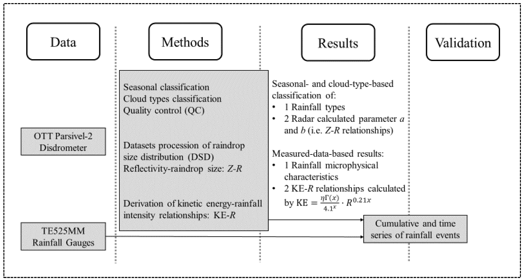
2. Materials and Methods
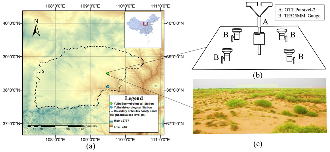
2.1. Observation Station and Disdrometer Datasets
2.2. Processing Microphysical Datasets from Disdrometer
2.3. Precipitation Types and Quality Control (QC)
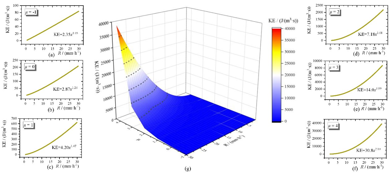
2.4. Derivation of KE-R Relationships
3. Results
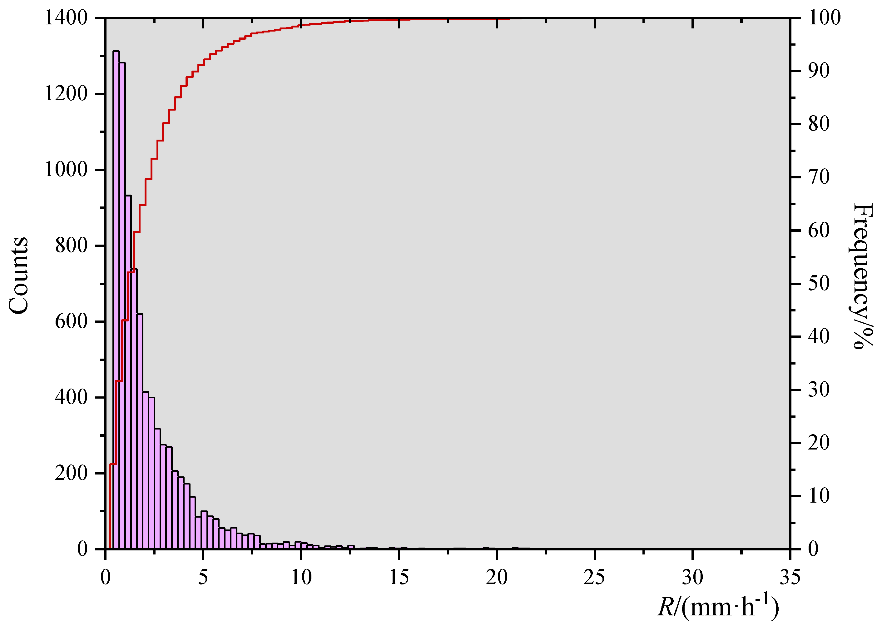
3.1. Data after Quality Control
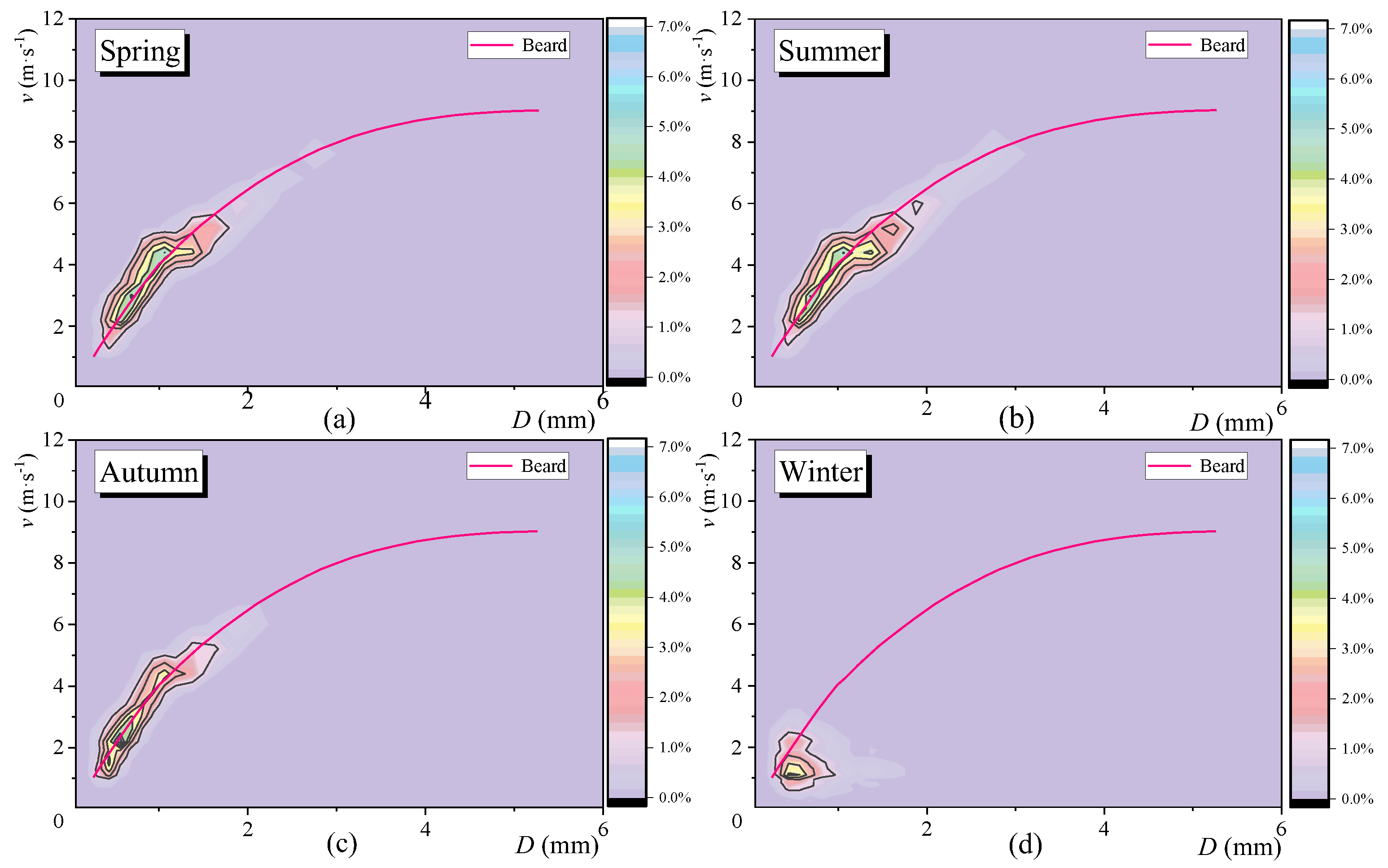
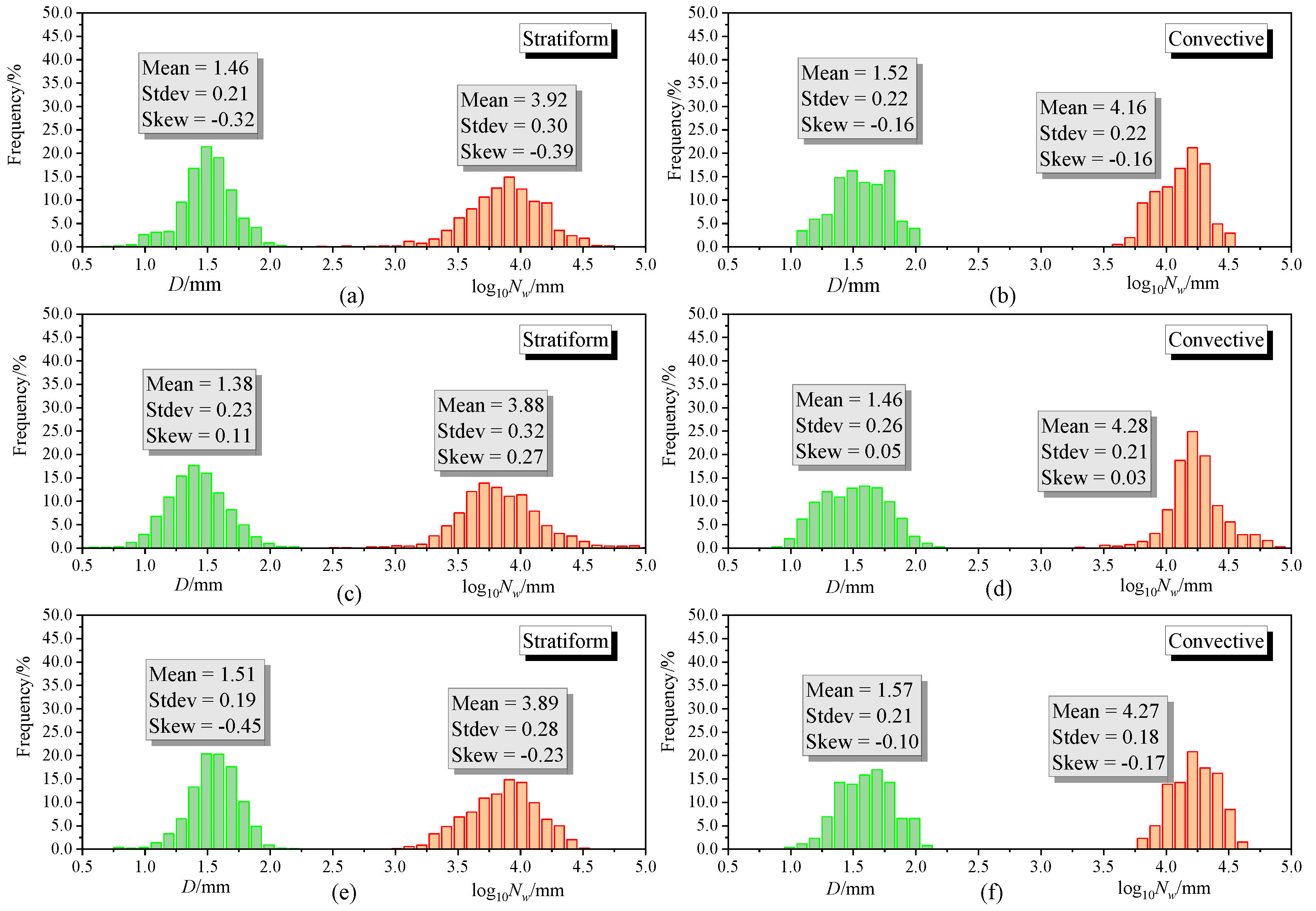
3.2. Microphysical Characteristics of Precipitation in Different Seasons
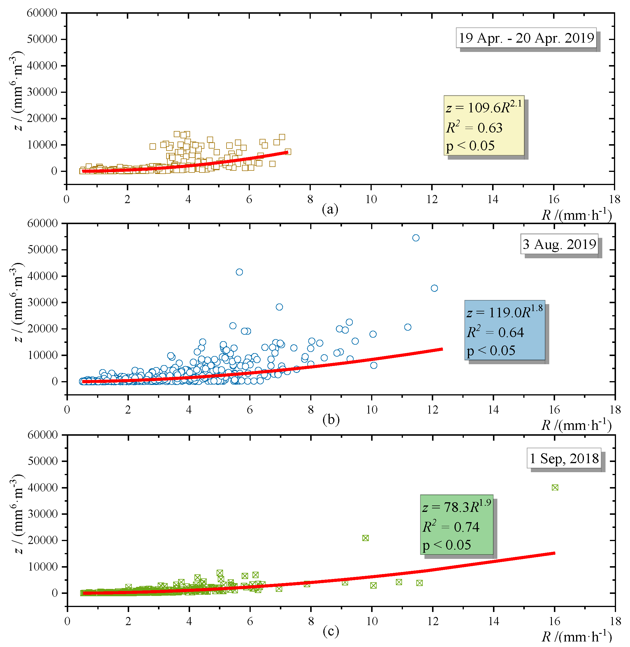
3.3. Z-R Relationships in Different Rainfall Events
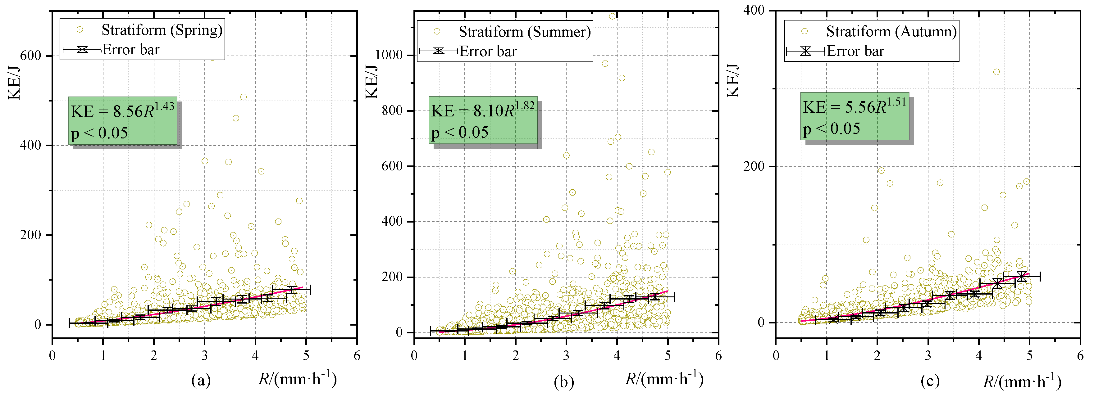
3.4. KE-R Relationships
4. Discussion
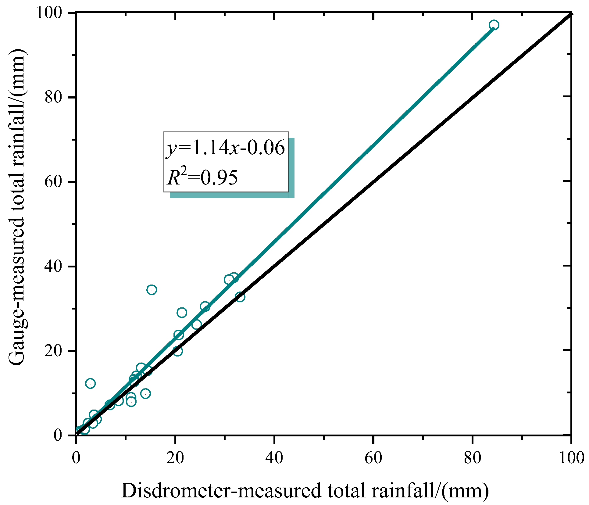
4.1. Uncertainty Analysis of Disdrometer-Measured Data
4.2. Comparison of Different Z-R Relationships
4.3. Sensitive Analysis of the Formula of KE-R Relationships
5. Conclusions
Author Contributions
Funding
Conflicts of Interest
Appendix A

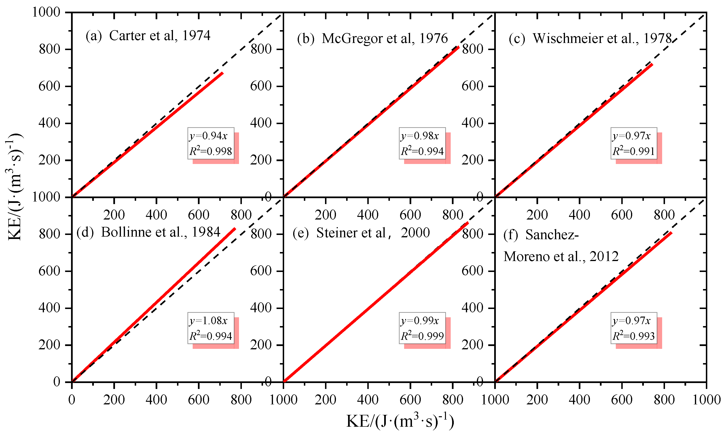
| References | KE-R Relationships (Originally Derived) | Form | KE-R Relationships (Based on Equation (18)) | μ |
|---|---|---|---|---|
| Carter et al., 1974 [68] | Polynomial | 1.09 | ||
| McGregor et al., 1976 [69] | Index | 1.30 | ||
| Wischmeier et al, 1978 [70] | Logarithm | 1.20 | ||
| Bollinne et al., 1984 [71] | Polynomial | 1.27 | ||
| Steiner et al., 2000 [67] | Power | 1.30 | ||
| Sanchez-Moreno et al., 2012 [72] | (10.09 + 12 logR)·R | Logarithm | 1.29 |

References
- Ding, B.; Yang, K.; Qin, J.; Wang, L.; Chen, Y.; He, X. The dependence of precipitation types on surface elevation and meteorological conditions and its parameterization. J. Hydrol. 2014, 513, 154–163. [Google Scholar] [CrossRef]
- Chen, B.J.; Yang, J.; Pu, J.P. Statistical Characteristics of Raindrop Size Distribution in the Meiyu Season Observed in Eastern China. J. Meteorol. Soc. Jpn. 2013, 91, 215–227. [Google Scholar] [CrossRef]
- Das, S.K.; Konwar, M.; Chakravarty, K.; Deshpande, S.M. Raindrop size distribution of different cloud types over the Western Ghats using simultaneous measurements from Micro-Rain Radar and disdrometer. Atmos. Res. 2017, 186, 72–82. [Google Scholar] [CrossRef]
- Hazenberg, P.; Leijnse, H.; Uijlenhoet, R. The impact of reflectivity correction and accounting for raindrop size distribution variability to improve precipitation estimation by weather radar for an extreme low-land mesoscale convective system. J. Hydrol. 2014, 519, 3410–3425. [Google Scholar] [CrossRef]
- Janapati, J.; Seela, B.K.; Reddy, M.V.; Reddy, K.K.; Lin, P.-L.; Rao, T.N.; Liu, C.-Y. A study on raindrop size distribution variability in before and after landfall precipitations of tropical cyclones observed over southern India. J. Atmos. Sol.-Terr. Phys. 2017, 159, 23–40. [Google Scholar] [CrossRef]
- Hazenberg, P.; Yu, N.; Boudevillain, B.; Delrieu, G.; Uijlenhoet, R. Scaling of raindrop size distributions and classification of radar reflectivity–rain rate relations in intense Mediterranean precipitation. J. Hydrol. 2011, 402, 179–192. [Google Scholar] [CrossRef]
- Waldvogel, A. TheN0Jump of Raindrop Spectra. J. Atmos. Sci. 1974, 31, 1067–1078. [Google Scholar] [CrossRef]
- Schönhuber, M.; Randeu, W.L.; Baptista, J.P.V.P. Application of the 2D-video-distrometer for weather radar data inversion. Phys. Chem. Earth Part B 2000, 25, 1037–1042. [Google Scholar] [CrossRef]
- Liu, X.; He, B.; Zhao, S.; Hu, S.; Liu, L. Comparative measurement of rainfall with a precipitation micro-physical characteristics sensor, a 2D video disdrometer, an OTT PARSIVEL disdrometer, and a rain gauge. Atmos. Res. 2019, 229, 100–114. [Google Scholar] [CrossRef]
- Zhang, A.; Hu, J.; Chen, S.; Hu, D.; Liang, Z.; Huang, C.; Xiao, L.; Min, C.; Li, H. Statistical Characteristics of Raindrop Size Distribution in the Monsoon Season Observed in Southern China. Remote Sens. 2019, 11, 432. [Google Scholar] [CrossRef]
- Raupach, T.H.; Berne, A. Correction of raindrop size distributions measured by Parsivel disdrometers, using a two-dimensional video disdrometer as a reference. Atmos. Meas. Tech. 2015, 8, 343–365. [Google Scholar] [CrossRef]
- Bringi, V.N.; Chandrasekar, V.; Hubbert, J.; Gorgucci, E.; Randeu, W.L.; Schoenhuber, M. Raindrop size distribution in different climatic regimes from disdrometer and dual-polarized radar analysis. J. Atmos. Sci. 2003, 60, 354–365. [Google Scholar] [CrossRef]
- Seliga, T.A.; Bringi, V.N. Potential use of the radar differential reflectivity measurements at orthogonal polarizations for measuring precipitation. J. Appl. Meteorol. 1976, 15, 69–76. [Google Scholar] [CrossRef]
- Sulochana, Y.; Rao, T.N.; Sunilkumar, K.; Chandrika, P.; Raman, M.R.; Rao, S.V.B. On the seasonal variability of raindrop size distribution and associated variations in reflectivity—Rainrate relations at Tirupati, a tropical station. J. Atmos. Sol.-Terr. Phys. 2016, 147, 98–105. [Google Scholar] [CrossRef]
- Wen, G.; Xiao, H.; Yang, H.L.; Bi, Y.H.; Xu, W.J. Characteristics of summer and winter precipitation over northern China. Atmos. Res. 2017, 197, 390–406. [Google Scholar] [CrossRef]
- Carollo, F.G.; Ferro, V.; Serio, M.A. Predicting rainfall erosivity by momentum and kinetic energy in Mediterranean environment. J. Hydrol. 2018, 560, 173–183. [Google Scholar] [CrossRef]
- Ji, L.; Chen, H.N.; Li, L.; Chen, B.J.; Xiao, X.; Chen, M.; Zhang, G.F. Raindrop Size Distributions and Rain Characteristics Observed by a PARSIVEL Disdrometer in Beijing, Northern China. Remote Sens. 2019, 11, 1479. [Google Scholar] [CrossRef]
- Angulo-Martínez, M.; Barros, A.P. Measurement uncertainty in rainfall kinetic energy and intensity relationships for soil erosion studies: An evaluation using PARSIVEL disdrometers in the Southern Appalachian Mountains. Geomorphology 2015, 228, 28–40. [Google Scholar] [CrossRef]
- Carollo, F.G.; Serio, M.A.; Ferro, V.; Cerdà, A. Characterizing rainfall erosivity by kinetic power - Median volume diameter relationship. Catena 2018, 165, 12–21. [Google Scholar] [CrossRef]
- Meshesha, D.T.; Tsunekawa, A.; Tsubo, M.; Haregeweyn, N.; Tegegne, F. Evaluation of kinetic energy and erosivity potential of simulated rainfall using Laser Precipitation Monitor. Catena 2016, 137, 237–243. [Google Scholar] [CrossRef]
- Abd Elbasit, M.A.M.; Yasuda, H.; Salmi, A.; Anyoji, H. Characterization of rainfall generated by dripper-type rainfall simulator using piezoelectric transducers and its impact on splash soil erosion. Earth Surf. Process. Landf. 2010, 35, 466–475. [Google Scholar] [CrossRef]
- Serio, M.A.; Carollo, F.G.; Ferro, V. Raindrop size distribution and terminal velocity for rainfall erosivity studies. A review. J. Hydrol. 2019, 576, 210–228. [Google Scholar] [CrossRef]
- Fan, Y.; Chen, Y.; Wei, J. An Analysis of Drought Features in Shaanxi Province. J. Xi’an Univ. Technol. 1996, 12, 200–206. [Google Scholar]
- Li, Y.; Cao, Z.; Long, H.; Liu, Y.; Li, W. Dynamic analysis of ecological environment combined with land cover and NDVI changes and implications for sustainable urban–rural development: The case of Mu Us Sandy Land, China. J. Clean. Prod. 2017, 142, 697–715. [Google Scholar] [CrossRef]
- Xie, Z.; Yang, H.; Lv, H. Study on the relationship between rainfall kinetic energy and rainfall intensity based on raindrop spectrum observations. Water Resour. Hydropower Eng. 2019. under review. [Google Scholar]
- Ulbrich, C.W. Natural Variations in the Analytical Form of the Raindrop Size Distribution. J. Clim. Appl. Meteorol. 1983, 22, 1764–1775. [Google Scholar] [CrossRef]
- Testud, J.; Oury, S.; Black, R.A.; Amayenc, P.; Dou, X.K. The concept of “normalized” distribution to describe raindrop spectra: A tool for cloud physics and cloud remote sensing. J. Appl. Meteorol. 2001, 40, 1118–1140. [Google Scholar] [CrossRef]
- Ulbrich, C.W.; Atlas, D. Rainfall microphysics and radar properties: Analysis methods for drop size spectra. J. Appl. Meteorol. 1998, 37, 912–923. [Google Scholar] [CrossRef]
- Tokay, A.; Wolff, D.B.; Petersen, W.A. Evaluation of the New Version of the Laser-Optical Disdrometer, OTT Parsivel2. J. Atmos. Ocean. Technol. 2014, 31, 1276–1288. [Google Scholar] [CrossRef]
- Zhang, H.; HE, H.; Zhang, Y.; Zeng, Q.; Bai, S. Parameter Characteristics Analysis of Raindrop Spectrum Fitting Models in Nanjing. Meteorol. Environ. Sci. 2017, 40, 77–84. [Google Scholar]
- Seela, B.K.; Janapati, J.; Lin, P.L.; Wang, P.K.; Lee, M.T. Raindrop Size Distribution Characteristics of Summer and Winter Season Rainfall Over North Taiwan. J. Geophys. Res.-Atmos. 2018, 123, 11602–11624. [Google Scholar] [CrossRef]
- Zhang, G.; Vivekanandan, J.; Brandes, E.A. The Shape–Slope Relation in Observed Gamma Raindrop Size Distributions: Statistical Error or Useful Information? J. Atmos. Ocean. Technol. 2003, 20, 1106–1119. [Google Scholar] [CrossRef]
- Low, T.B.; List, R. Collision, Coalescence and Breakup of Raindrops. Part I: Experimentally Established Coalescence Efficiencies and Fragment Size Distributions in Breakup. J. Atmos. Sci. 1982, 39, 1591–1606. [Google Scholar] [CrossRef]
- Tokay, A.; Bashor, P.G. An Experimental Study of Small-Scale Variability of Raindrop Size Distribution. J. Appl. Meteorol. Clim. 2010, 49, 2348–2365. [Google Scholar] [CrossRef]
- Zhou, L.M.; Zhang, H.S.; Wang, J.; Wang, Q.; Chen, X.L. Raindrop Spectral Charcteristics of Mixed-cloud Precipitation in Shandong Province. Meteorol. Sci. Technol. 2010, 38, 73–77. [Google Scholar]
- Li, H.; Yin, Y.; Shan, Y.; Jin, Q. Statistical Characteristics of Raindrop Size Distribution for Stratiform and Convective Precipitation at Different Altitudes in Mt. Huangshan. Chin. J. Atmos. Sci. 2018, 42, 268–280. [Google Scholar]
- Chen, C.; Yin, Y.; Chen, B.J. Raindrop Size Distribution at Different Altitudes in Mt. Huang. Trans. Atmos. Sci. 2015, 38, 388–395. [Google Scholar] [CrossRef]
- Kinnell, P. Rainfall Intensity-Kinetic Energy Relationships for Soil Loss Prediction 1. Soil Sci. Soc. Am. J. 1981, 45, 153–155. [Google Scholar] [CrossRef]
- Atlas, D.; Ulbrich, C.W. Path-and area-integrated rainfall measurement by microwave attenuation in the 1–3 cm band. J. Appl. Meteorol. 1977, 16, 1322–1331. [Google Scholar] [CrossRef]
- Marshall, J.S.; Palmer, W.M.K. The Distribution of Raindrops with Size. J. Meteorol. 1948, 5, 165–166. [Google Scholar] [CrossRef]
- Uijlenhoet, R.; Stricker, J. A consistent rainfall parameterization based on the exponential raindrop size distribution. J. Hydrol. 1999, 218, 101–127. [Google Scholar] [CrossRef]
- Lane, J.; Hackathorn, M.; Kewley, J.; Madore, M.; May, M.; Briggs, C.; DeLeon Springs, F. A method for estimating 3-D spatial variations of rainfall drop size distributions over remote ocean areas. Presented at the Fifth International Conference on Remote Sensing for Marine and Coastal Environments, San Diego, CA, USA, 5–7 October 1998; p. 7. [Google Scholar]
- Ochou, A.D.; Nzeukou, A.; Sauvageot, H. Parametrization of drop size distribution with rain rate. Atmos. Res. 2007, 84, 58–66. [Google Scholar] [CrossRef]
- Li, P.; Sun, X.; Zhao, X. Analysis of precipitation and potential evapotranspiration in arid and semi-arid area of China in recent 50 years. J. Arid Land Res. Environ. 2012, 7, 57–63. [Google Scholar]
- Beard, K.V. Terminal Velocity and Shape of Cloud and Precipitation Drops Aloft. J. Atmos. Sci. 1976, 33, 851–864. [Google Scholar] [CrossRef]
- Hunt, W.F.; Jarrett, A.R.; Smith, J.T.; Sharkey, L.J. Evaluating bioretention hydrology and nutrient removal at three field sites in North Carolina. J. Irrig. Drain. Eng. 2006, 132, 600–608. [Google Scholar] [CrossRef]
- Hunter, S.M. WSR-88D radar rainfall estimation: Capabilities, limitations and potential improvements. Natl. Weather Dig. 1996, 20, 26–38. [Google Scholar]
- Austin, P.M. Relation between Measured Radar Reflectivity and Surface Rainfall. Mon. Weather Rev. 1987, 115, 1053–1071. [Google Scholar] [CrossRef]
- Sauvageot, H. Rainfall Measurement by Radar—A Review. Atmos. Res. 1994, 35, 27–54. [Google Scholar] [CrossRef]
- Wilson, J.W.; Brandes, E.A. Radar measurement of rainfall—A summary. Bull. Am. Meteorol. Soc. 1979, 60, 1048–1060. [Google Scholar] [CrossRef]
- Zhang, P.; Du, B.; Dai, T.P. Radar Meteorology; China Meteorological Press: Beijing, China, 2001.
- Petan, S.; Rusjan, S.; Vidmar, A.; Mikos, M. The rainfall kinetic energy-intensity relationship for rainfall erosivity estimation in the mediterranean part of Slovenia. J. Hydrol. 2010, 391, 314–321. [Google Scholar] [CrossRef]
- Battaglia, A.; Rustemeier, E.; Tokay, A.; Blahak, U.; Simmer, C. PARSIVEL Snow Observations: A Critical Assessment. J. Atmos. Ocean. Technol. 2010, 27, 333–344. [Google Scholar] [CrossRef]
- Liu, X.C.; Gao, T.C.; Liu, L. A comparison of rainfall measurements from multiple instruments. Atmos. Meas. Tech. 2013, 6, 1585–1595. [Google Scholar] [CrossRef]
- Kang, L. A Study on Dynamic Correction for Radar-Derived Quantitation Precipitation Estimation Based on the Optimal Z-I Relationship; Lanzhou University: Lanzhou, China, 2014. [Google Scholar]
- Yuan, X.; Ni, G.; Pan, A.; Wei, L. NEXRAD Z-R Power Relationship in Beijing Based on Optimization Algorithm. J. Chin. Hydrol. 2010, 30, 1–6. [Google Scholar]
- Zhang, P.; Dai, T.; WANG, D.; Lin, B. Derivation of The Z-I Relationship by Optimization and The Accuracy in The Quantitative Rainfall Measurement. Sci. Meteorol. Sin. 1992, 12, 333–338. [Google Scholar]
- Marshall, J.S.; Langille, R.C.; Palmer, W.M.K. Measurement of Rainfall by Radar. J. Meteorol. 1947, 4, 186–192. [Google Scholar] [CrossRef]
- Chen, Q.; Niu, S.; Zhang, Y.; Xu, F. Z-R Relationship from the Particle Size and Velocity (Parsivel) optical disdrometer and its Application in Estimating Areal Rainfall. In Proceedings of the 2008 2nd International Conference on Bioinformatics and Biomedical Engineering, Shanghai, China, 16–18 May 2008. [Google Scholar]
- Marzuki; Randeu, W.L.; Kozu, T.; Shimomai, T.; Hashiguchi, H.; Schönhuber, M. Raindrop axis ratios, fall velocities and size distribution over Sumatra from 2D-Video Disdrometer measurement. Atmos. Res. 2013, 119, 23–37. [Google Scholar] [CrossRef]
- Blanchard, D.C. Raindrop Size-Distribution in Hawaiian Rains. J. Meteorol. 1953, 10, 457–473. [Google Scholar] [CrossRef]
- Sivaramakrishnan, M.V. Studies of raindrop size characteristics in different types of tropical rain using a simple recorder. Indian J. Meteorol. Geophys. 1961, 12, 189–217. [Google Scholar]
- Yakubu, M.L.; Yusop, Z.; Fulazzaky, M.A. The influence of rain intensity on raindrop diameter and the kinetics of tropical rainfall: Case study of Skudai, Malaysia. Hydrolog. Sci. J. 2016, 61, 944–951. [Google Scholar] [CrossRef]
- Takeuchi, D. Characterization of raindrop size distributions. In Proceedings of the Conference on Cloud Physics and Atmospheric Electricity, Issaquah, WA, USA, 31 July–4 August 1978; pp. 154–161. [Google Scholar]
- Teng, X. Sensitivity of the W Band Airborne Cloud Radar Reflectivity Factor Z to Cloud Parameters; Nanjing University of Information Science and Technology: Nanjing, China, 2011. [Google Scholar]
- Park, S.W.; Mitchell, J.K.; Bubenzer, G.D. An analysis of splash erosion mechanics. In Proceedings of the ASAE 1980 Winter Meeting, Chicago, IL, USA, 4 December 1980; p. 27. [Google Scholar]
- Steiner, M.; Smith, J.A. Reflectivity, rain rate, and kinetic energy flux relationships based on raindrop spectra. J. Appl. Meteorol. 2000, 39, 1923–1940. [Google Scholar] [CrossRef]
- Carter, C.E.; Greer, J.D.; Braud, H.J.; Floyd, J.M. Raindrop Characteristics in South Central United-States. Trans. ASAE 1974, 17, 1033–1037. [Google Scholar] [CrossRef]
- McGregor, K.C.; Mutchler, C.K. Status of the R factor in northern Mississippi. In Soil Erosion: Prediction and Control, Soil Conservation Soc. Amer.; Nature: UK, 1976; pp. 135–142. [Google Scholar]
- Wischmeier, W.H.; Smith, D.D. Predicting Rainfall Erosion Losses: A Guide to Conservation Planning; Science and Education Administration, US Department of Agriculture: Washington, WA, USA, 1978; Volume 537.
- Bollinne, A.; Florins, P.; Hecq, P.; Homerin, D.; Renard, V. Etude de l’énergie des pluies en climat tempéré océanique d’Europe Atlantique. Zeitschrift für Geomorphologie 1984, 49, 27–35. [Google Scholar]
- Sanchez-Moreno, J.F.; Mannaerts, C.M.; Jetten, V.; Loffler-Mang, M. Rainfall kinetic energy-intensity and rainfall momentum-intensity relationships for Cape Verde. J. Hydrol. 2012, 454, 131–140. [Google Scholar] [CrossRef]


| Rainfall Characteristics | Spring (March–May) | Summer (June–August) | Autumn (September–November) | Winter (December–February) |
|---|---|---|---|---|
| Total time with data recorded (min) | 3387 | 7019 | 4230 | 116 |
| Total time of stratiform rain (min) | 1813 | 3431 | 2126 | 18 |
| Total time of convective rain (min) | 86 | 563 | 147 | - |
| Percentage of stratiform rain (%) | 95.5 | 85.9 | 93.5 | 100 |
| Percentage of convective rain (%) | 4.5 | 14.1 | 6.5 | - |
| Percentage of rainfall time over the season (%) | 1.4 | 3.0 | 1.7 | ≈0 |
| Maximum rainfall intensity | 12.6 | 33.7 | 21.2 | 1.1 |
| Average | 2.0 | 2.6 | 2.0 | 0.7 |
| Median Rm | 1.9 | 1.9 | 1.6 | 0.7 |
| Precipitation Accumulation Ptotal (mm) | 76.7 | 236.9 | 105.9 | - * |
| Standard deviation of rainfall intensity R | 1.6 | 2.8 | 1.8 | 0.15 |
| 60.3 | 58.8 | 66.4 | 100 | |
| 35.1 | 27.1 | 27.1 | - | |
| 4.2 | 11.3 | 6.0 | - | |
| 0.4 | 2.8 | 0.5 | - |
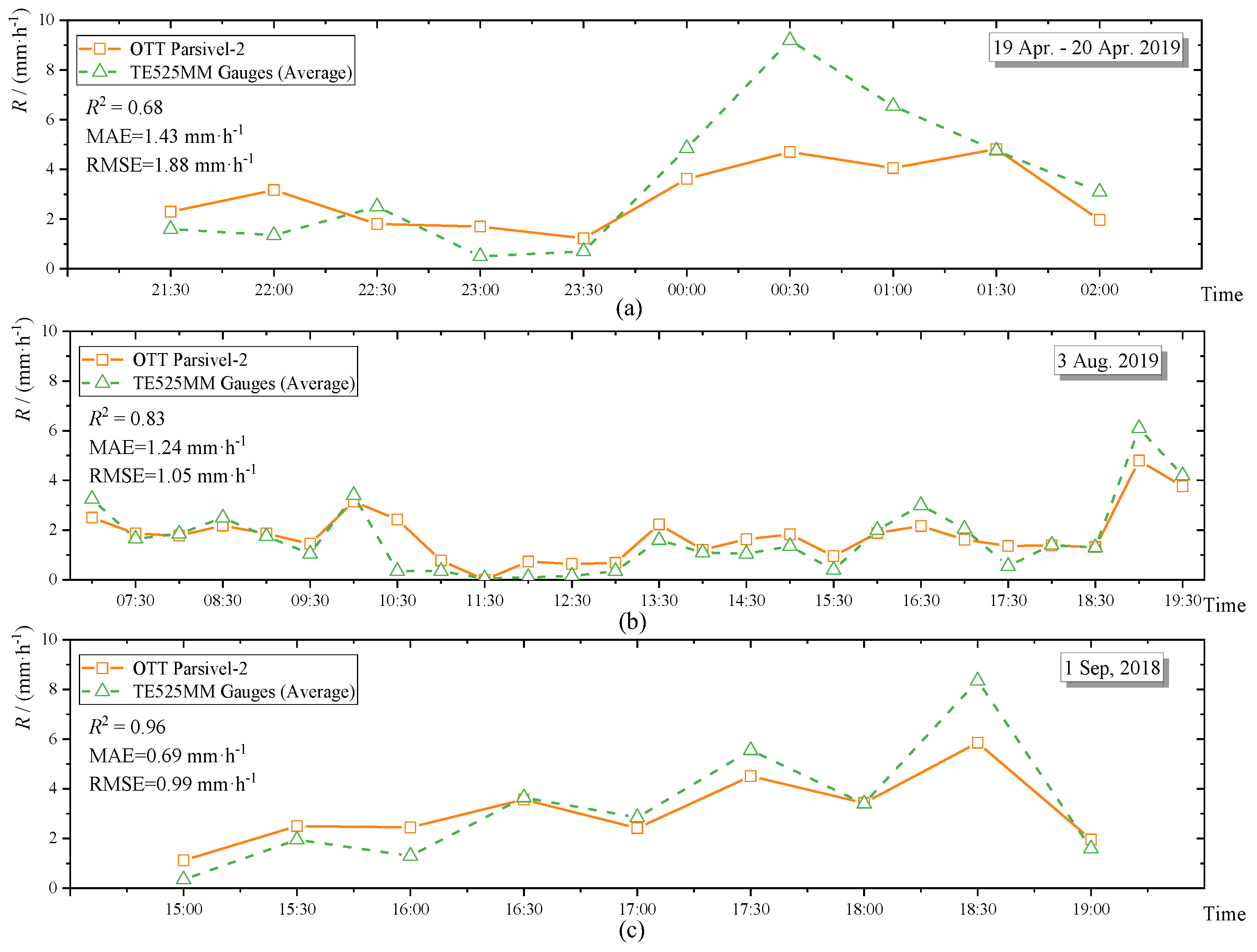
| Rainfall Number | Rainfall Time | Season | * | ** | Duration | S/C Records |
|---|---|---|---|---|---|---|
| Event 1 | 19–20 April 2019 | Spring | 3.36 | 3.51 | 4 h 30 min | 225/34 |
| Event 2 | 3 August 2019 | Summer | 1.65 | 1.78 | 12 h 30 min | 897/101 |
| Event 3 | 1 September 2018 | Autumn | 3.09 | 3.22 | 4 h | 241/32 |
| Reference [57,58,59,60,61,62] | Precipitation Time/Season | Location | Measurement Method | Z-R relationships | Rainfall Type |
|---|---|---|---|---|---|
| Zhang et al., 1992 | July in 1981 | Jiangsu, Eastern China | Digital Radar | Heavy rain | |
| Marshall et al., 1947 | Summer in 1946 | Canada | MHF Radar | Thunderstorm | |
| Chen et al., 2008 | 15 July–7 August in 2007 | Leizhou Peninsula, China | Parsivel Disdrometer | Convective rain Mixed-cloud rain | |
| Marzuki et al., 2013 | 2006–2007 | Kototabang, West Sumatra, Indonesia | 2D-Video Disdrometer | Stratiform rain | |
| Hazenberg et al., 2011 | 14 September 2006 | Cévennes-Vivarais region, France | OTT/Parsivel Disdrometer | Stratiform rain | |
| Blanchard, 1953 | October in 1951–August in 1952 | Hawaii, USA | Filter-paper | Thunderstorm | |
| Sivaramakrishnan, 1961 | November in 1958 | India | Filter-paper | Thunderstorm |
| Spring | Summer | Autumn | Total Year | |
|---|---|---|---|---|
| 4.10 | 4.68 | 3.83 | 4.29 | |
| 3.88 | 3.79 | 3.97 | 3.88 |
© 2020 by the authors. Licensee MDPI, Basel, Switzerland. This article is an open access article distributed under the terms and conditions of the Creative Commons Attribution (CC BY) license (http://creativecommons.org/licenses/by/4.0/).
Share and Cite
Xie, Z.; Yang, H.; Lv, H.; Hu, Q. Seasonal Characteristics of Disdrometer-Observed Raindrop Size Distributions and Their Applications on Radar Calibration and Erosion Mechanism in a Semi-Arid Area of China. Remote Sens. 2020, 12, 262. https://doi.org/10.3390/rs12020262
Xie Z, Yang H, Lv H, Hu Q. Seasonal Characteristics of Disdrometer-Observed Raindrop Size Distributions and Their Applications on Radar Calibration and Erosion Mechanism in a Semi-Arid Area of China. Remote Sensing. 2020; 12(2):262. https://doi.org/10.3390/rs12020262
Chicago/Turabian StyleXie, Zongxu, Hanbo Yang, Huafang Lv, and Qingfang Hu. 2020. "Seasonal Characteristics of Disdrometer-Observed Raindrop Size Distributions and Their Applications on Radar Calibration and Erosion Mechanism in a Semi-Arid Area of China" Remote Sensing 12, no. 2: 262. https://doi.org/10.3390/rs12020262
APA StyleXie, Z., Yang, H., Lv, H., & Hu, Q. (2020). Seasonal Characteristics of Disdrometer-Observed Raindrop Size Distributions and Their Applications on Radar Calibration and Erosion Mechanism in a Semi-Arid Area of China. Remote Sensing, 12(2), 262. https://doi.org/10.3390/rs12020262