SAR Interferometric Baseline Refinement Based on Flat-Earth Phase without a Ground Control Point

Abstract

Interferometric baseline estimation is a key procedure of interferometric synthetic aperture radar (SAR) data processing. The error of the interferometric baseline affects not only the removal of the flat-earth phase, but also the transformation coefficient between the topographic phase and elevation, which will affect the topographic phase removal for differential interferometric SAR (D-InSAR) and the accuracy of the final generated digital elevation model (DEM) product for interferometric synthetic aperture (InSAR). To obtain a highly accurate interferometric baseline, this paper firstly investigates the geometry of InSAR imaging and establishes a rigorous relationship between the interferometric baseline and the flat-earth phase. Then, a baseline refinement method without a ground control point (GCP) is proposed, where a relevant theoretical model and resolving method are developed. Synthetic and real SAR datasets are used in the experiments, and a comparison with the conventional least-square (LS) baseline refinement method is made. The results demonstrate that the proposed method exhibits an obvious improvement over the conventional LS method, with percentages of up to 51.5% in the cross-track direction. Therefore, the proposed method is effective and advantageous.

1. Introduction

During the past two decades, the interferometric synthetic aperture radar (InSAR) has been gradually matured in terms of theory and widely used in topographic mapping [1] and surface deformation monitoring [2]. For example, the shuttle radar topography mission (SRTM) data forms a popular digital elevation model (DEM, a surface model representing ground elevation as an ordered set of numerical arrays), which is acquired by airborne SAR [3]. Recently, the application fields of InSAR have been expanded from earthquakes, volcanic eruptions, ground subsidence, and other large-scale macroscopic monitoring to infrastructure monitoring, such as bridges, dams, and buildings, as well as high-accuracy 3-D urban reconstruction [4,5,6], the prospect of which is very broad.

However, the accuracy of InSAR is affected by a variety of errors, such as atmospheric delay error, DEM error, random phase error, and baseline estimation error. Among such errors, interferometric baseline estimation error systematically and seriously affects the accuracy of InSAR measurement [7]. The error of the interferometric baseline affects not only the removal of the flat-earth phase, but also the transformation coefficient between the topographic phase and elevation, which will affect the topographic phase removal for D-InSAR and the accuracy of the finally generated DEM product for InSAR. The present methods of initial baseline estimation make it difficult to obtain high-accuracy baseline estimations due to factors such as the precision of the satellite orbit state vector.

The baseline estimation method based on the satellite orbit state vector utilizes the difference in instantaneous satellite coordinates to obtain the interferometric baseline estimation, while it is directly affected by the precision of the satellite orbit state vector. According to the law of error propagation [8], the accuracy of the results is lower than that of the satellite orbit state vector. Several SAR satellites are equipped with global navigation satellite system (GNSS) positioning devices, such as TerraSAR and COSMO-SkyMed, the precise orbit state vector accuracy of which is about 5 cm and the fast track accuracy of which is only 10 cm [9]. The orbit state vector accuracy of ERS-1/2 and ENVISAT (Environmental Satellite) is as low as 10~15 cm [10,11], while that of ALOS (Advanced Land Observing Satellite)/PALSAR (Phased Array type L-band Synthetic Aperture Radar) is even worse [12].

The baseline estimation method based on image registration offset [13,14,15] converts the range offset estimation into slant-range difference, using the relationship between the slant-range offsets and distance between the master image and slave image, and calculates the interferometric baseline estimation with SAR imaging geometry. Restricted by the accuracy of the image registration algorithm, the accuracy of baseline estimation is relatively low, and is generally at a meter or decimeter level [15]. For example, if the accuracy of SAR image registration reaches 1/10 pixel, then that of the slant-range difference is about 30 cm for TerraSAR with a 3 m resolution. Therefore, the accuracy of interferometric baseline estimation is low.

The baseline estimation method based on the visible fringe rate is derived from the paper on the beam transform published by the Italian researcher Gatelli in 1994 [16]. Gatelli et al. proved that the interferometric baseline can be determined by the relationship between the fringe frequency and SAR spatial geometry. Hence, once the fringe frequency can be accurately obtained, the SAR interferometric baseline estimation can be calculated. Many researchers have carried out a lot of research on this method, such as Wegmuller [13], Li Xinwu [17], Tang Xiaoqing [18], Fan Hongdong [19], Xu Huaping [20], and so on. In practice, due to the lack of accurate terrain slope information, we usually select flat terrain to estimate the fringe frequency and interferometric baseline. However, some defects still exist in this method: on the one hand, it is difficult to search flat terrain in some cases, and on the other hand, the calculation accuracy is affected by the window size that is adopted by fast Fourier transform (FFT) for obtaining the fringe frequency, as well as the interferometric phase within the window. The SAR interferometric baseline in the whole interferogram is not a fixed value, which means that it changes over time. This means that the method has to calculate the fringe frequency based on the interferogram within a certain window (e.g., 512 × 512 pixels) to get the average baseline of the selected area. The larger the window one adopts, the more accurate the estimation is, while the deviation from the local real baseline is larger, caused by more interferogram samples being contained. Conversely, when the estimation window is small, the deviation between the baseline estimation and local real value can be smaller, but its accuracy is affected by the interferogram.

According to an analysis of the existing methods for SAR interferometric baseline estimation, we can see that all of these methods have inherent defects, meaning that they cannot obtain highly accurate baseline estimations. To remove the phase error caused by inaccurate baseline estimation, there are two methods available, namely, interferometric phase error correction [21] (e.g., planar polynomial fitting) and precise baseline estimation [22]. It has been proven that planar polynomial fitting can just subtract the trend of the baseline error from the interferogram, while the topographic phase residuals caused by phase error still remain [23]. This part of the error is associated with the elevation and can easily be considered as the atmospheric error related to elevation. Therefore, an interferometric baseline refinement procedure is necessary for real InSAR data processing. Small et al. [22], Joughin et al. [24], and Kimura et al. [25] have successively proposed a baseline refinement method based on the ground control point (GCP). The method establishes the observation equation on the basis of the known unwrapped phase and GCP elevations and computes the baseline parameters using the least-squares algorithm, so the method is called the baseline refinement with least-squares (LS) (hereinafter referred to as the LS method). However, in many cases, we cannot obtain the ground control points of the interest area. By taking advantage of the geometric relationship as the slant-range ellipsoid, Doppler cone, and earth ellipsoid intersect at the GCP, Liu et al. [26] calculated the elevation of GCP with iterations and then computed the baseline estimation based on LS. However, the accuracy of the iterative calculation of GCP is limited.

In recent years, some researchers have combined SAR interferometric baseline refinement with multi-temporal InSAR and proposed corresponding methods [27,28]. However, when calculating radar vectors in line of sight (LOS), the baseline refinement models they have used are highly dependent on the precision of ground elevation information, which affects the accuracy of the baseline refinement results to some extent.

In order to obtain an interferometric baseline with a high accuracy and avoid the dependence of the refinement model on ground elevation, this paper firstly investigates the geometry of InSAR imaging and analyzes the rigorous geometric relationship between the interferometric baseline and flat-earth phase in detail. Then, a baseline refinement method without GCPs is proposed and the geometry is converted from precise baseline estimation to an InSAR flat-earth phase. We develop the theoretical model and resolving method. Synthetic and real SAR datasets are used in the experiments. Compared with the conventional LS method, the proposed method is more effective and advantageous.

2. SAR Interferometric Baseline Model

Since the orbits of an SAR satellite do not coincide with each other at the time of imaging, we refer to the spatial vector consisting of the satellite platform orbital positions as the SAR interferometric baseline, i.e.,

$$\begin{array}{ll}\overrightarrow{B}{(t_M)}_{XYZ}& =\overrightarrow{O}(t_S)-\overrightarrow{O}(t_M)\\ & ={\left[X(t_S)-X(t_M),Y(t_S)-Y(t_M),Z(t_S)-Z(t_M)\right]}^T\\ & ={\left[B_x(t_M),B_y(t_M),B_z(t_M)\right]}^T\end{array},$$

(1)

where $O(·)=\left[X(·),Y(·),Z(·)\right]$ is the 3-D spatial coordinate vector of the SAR sensor platform at ground point P; $t_M$ and $t_S$ are the acquisition times of point P in the master and slave image, respectively; and $B_x$, $B_y$, and $B_z$ are the baseline components in X, Y, and Z directions, respectively.

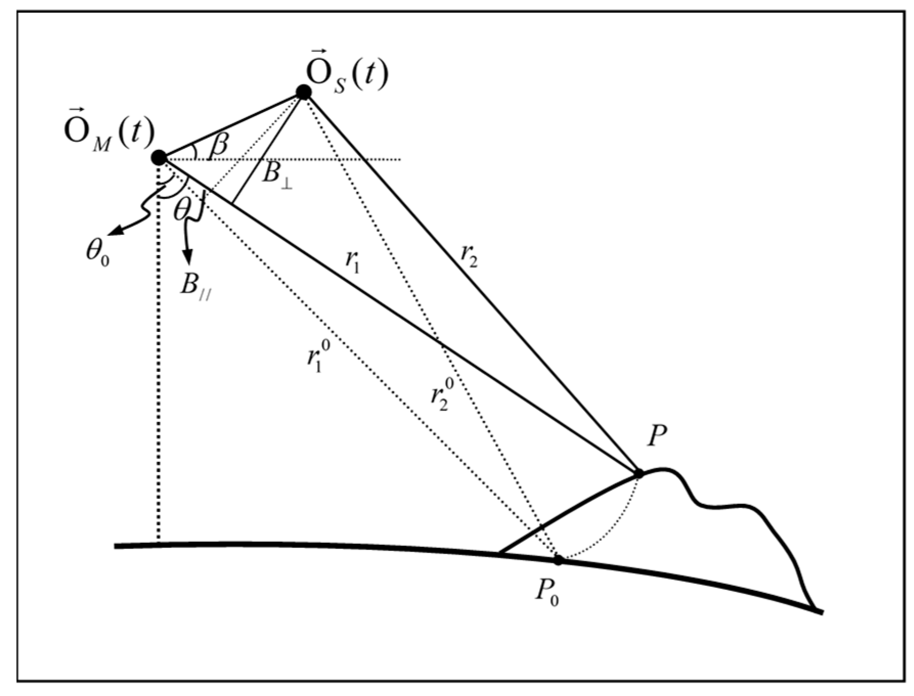
As shown in Figure 1, the baseline can be represented as the parallel component along the LOS of the radar and the perpendicular component perpendicular to the LOS, i.e.,

$$B_{//}\approx \left|\overrightarrow{B}\right|·\sin \left(\theta -\beta \right)$$

(2)

$$B_{\perp }\approx \left|\overrightarrow{B}\right|·\cos \left(\theta -\beta \right).$$

(3)

It should be noted that the precise look angle $\theta$ is required for this baseline decomposition, while its calculation depends on the ground elevation. Here, we introduce an alternative baseline representation independent of ground elevation for subsequent theoretical derivation.

We adopt an SAR platform-fixed coordinate system, TCN (see bibliography [22,26] for details, T, Along-Track, the flight direction of satellite; C, Cross-Track, perpendicular to the plane consisting of T and N to meet the left-handed coordinate system; N, Normal-Direction, the direction from the center of the earth towards the satellite). Then, the transformation matrix from the earth-fixed coordinate to the TCN coordinate is formed by

$$T={\left[\overrightarrow{t},\overrightarrow{c},\overrightarrow{n}\right]}^T,$$

(4)

where $\overrightarrow{t}$, $\overrightarrow{c}$, and $\overrightarrow{n}$, represent the unit vectors of the T axis, C axis, and N axis in the earth-fixed coordinate, respectively [26]. The baseline can be converted to the TCN coordinate by

$$\overrightarrow{B}{(t)}_{TCN}=T·\overrightarrow{B}{(t)}_{XYZ}={\left[B_t(t),B_c(t),B_n(t)\right]}^T.$$

(5)

As we can see from Formula (5), the decomposition of the baseline in the TCN coordinate does not depend on the ground elevation, which will be adopted for the subsequent theoretical derivation.

Since the SAR interferometric baseline in the whole interferogram is not a fixed value, we can model the baseline components using linear formulas, i.e.,

$$B_c(t)=B_{c,0}+{\alpha }_c·t$$

(6)

$$B_n(t)=B_{n,0}+{\alpha }_n·t,$$

(7)

where $B_{c,0}$ and $B_{n,0}$ respectively represent the components in the directions C and N of the SAR interferometric baseline model at the reference time, namely the baseline constants. We usually set the image centers as the time reference points (then $B_{c,0}$ and $B_{n,0}$ are the components of the image center baseline in the directions C and N, respectively). ${\alpha }_c$ and ${\alpha }_n$ are the baseline change rates in the directions C and N, respectively. $t$ is the time at which the point was acquired relative to the reference time. $B_{c,0}$, $B_{n,0}$, ${\alpha }_c$, and ${\alpha }_n$ are unknown model parameters. Here, taking the image co-registration into account, the baseline component in T has been eliminated, which means $B_t=0$ and is no longer within consideration.

3. Improvement of the Goldstein Filter By the Coefficient of Variation

3.1. Coefficient of Variation

According to SAR imaging geometry (see Figure 1), the unwrapped flat-earth phase can be expressed by

$${\varphi }_{flat,unw}=\frac{4\pi }{\lambda }\left(\left|{\overrightarrow{r}}_1^0\right|-\left|{\overrightarrow{r}}_2^0\right|\right)-{\varphi }_0,$$

(8)

where $\lambda$ is the radar wavelength, $\overrightarrow{r}={\left[r_t,r_c,r_n\right]}^T$ is the decomposition of the slant range in TCN coordinates, and ${\varphi }_0$ is the unwrapped flat-earth phase of the reference point. Based on Cosine law, we can get

$$\left|{\overrightarrow{r}}_2^0\right|=\sqrt{{\left|{\overrightarrow{r}}_1^0\right|}^2+{\left|\overrightarrow{B}\right|}^2-2{\overrightarrow{r}}_1^0·\overrightarrow{B}}$$

(9)

and

$$\overrightarrow{B}={[0,B_c,B_n]}^T=0·\overrightarrow{t}+B_c·\overrightarrow{c}+B_n·\overrightarrow{n}.$$

(10)

Given N observations, let the observation vector $L={\varphi }_{flat,unw}$ with the size of $N\times 1$. $X=\left[B_{c,0},B_{n,0},{\alpha }_c,{\alpha }_n,{\varphi }_0\right]$ is the parameter vector to be resolved. Additionally, $f\left(X\right)=4\pi ·\left(\left|{\overrightarrow{r}}_1{}^0\right|-\left|{\overrightarrow{r}}_2{}^0\right|\right)/\lambda -{\varphi }_0$ is the non-linear equation of parameter vector X. Then, Equation (8) is rewritten into the observation equation as

$$L=f(X)+\Delta ,$$

(11)

where $\Delta$ is the error vector of observation $L$. Equation (11) is a non-linear equation, and in this paper, it will be transformed into a linear one. By expanding Equation (11) into Taylor Series at $X^0={\left[B_{c,0}^0,B_{n,0}^0,{\alpha }_c^0,{\alpha }_n^0,0\right]}^T$, retaining zero- and first-order items, and writing it as an error equation, we can get

$$V={\frac{\partial f(X)}{\partial X}|}_{X=X^0}·x-l,$$

(12)

where $x=X-X^0$ and $l=L-f\left(X^0\right)$.

Let

$$\begin{gathered} A={\frac{\partial f(X)}{\partial X}|}_{X=X^0}=\left[\begin{array}{ccccc}{\frac{\partial f_1(X)}{\partial B_{c,0}}|}_{X=X^0}& {\frac{\partial f_1(X)}{\partial B_{n,0}}|}_{X=X^0}& {\frac{\partial f_1(X)}{\partial {\alpha }_c}|}_{X=X^0}& {\frac{\partial f_1(X)}{\partial {\alpha }_n}|}_{X=X^0}& {\frac{\partial f_1(X)}{\partial {\varphi }_0}|}_{X=X^0}\\ {\frac{\partial f_2(X)}{\partial B_{c,0}}|}_{X=X^0}& {\frac{\partial f_2(X)}{\partial B_{n,0}}|}_{X=X^0}& {\frac{\partial f_2(X)}{\partial {\alpha }_c}|}_{X=X^0}& {\frac{\partial f_2(X)}{\partial {\alpha }_n}|}_{X=X^0}& {\frac{\partial f_2(X)}{\partial {\varphi }_0}|}_{X=X^0}\\ ⋮& ⋮& ⋮& ⋮& ⋮\\ {\frac{\partial f_N(X)}{\partial B_{c,0}}|}_{X=X^0}& {\frac{\partial f_N(X)}{\partial B_{n,0}}|}_{X=X^0}& {\frac{\partial f_N(X)}{\partial {\alpha }_c}|}_{X=X^0}& {\frac{\partial f_N(X)}{\partial {\alpha }_n}|}_{X=X^0}& {\frac{\partial f_N(X)}{\partial {\varphi }_0}|}_{X=X^0}\end{array}\right] \\ =-\frac{4\pi }{\lambda }·\left[\begin{array}{ccccc}\frac{B_{c,1}-{\left|{\overrightarrow{r}}_1^0\right|}_1·\sin {\theta }_{0,1}}{{\left|{\overrightarrow{r}}_2^0\right|}_1}& \frac{B_{n,1}-{\left|{\overrightarrow{r}}_1^0\right|}_1·\cos {\theta }_{0,1}}{{\left|{\overrightarrow{r}}_2^0\right|}_1}& \frac{\left(B_{c,1}-{\left|{\overrightarrow{r}}_1^0\right|}_1·\sin {\theta }_{0,1}\right)·t_1}{{\left|{\overrightarrow{r}}_2^0\right|}_1}& \frac{\left(B_{n,1}-{\left|{\overrightarrow{r}}_1^0\right|}_1·\cos {\theta }_{0,1}\right)·t_1}{{\left|{\overrightarrow{r}}_2^0\right|}_1}& \frac{\lambda }{4\pi }\\ \frac{B_{c,2}-{\left|{\overrightarrow{r}}_1^0\right|}_2·\sin {\theta }_{0,2}}{{\left|{\overrightarrow{r}}_2^0\right|}_2}& \frac{B_{n,2}-{\left|{\overrightarrow{r}}_1^0\right|}_2·\cos {\theta }_{0,2}}{{\left|{\overrightarrow{r}}_2^0\right|}_2}& \frac{\left(B_{c,2}-{\left|{\overrightarrow{r}}_1^0\right|}_2·\sin {\theta }_{0,2}\right)·t_2}{{\left|{\overrightarrow{r}}_2^0\right|}_2}& \frac{\left(B_{n,2}-{\left|{\overrightarrow{r}}_1^0\right|}_2·\cos {\theta }_{0,2}\right)·t_2}{{\left|{\overrightarrow{r}}_2^0\right|}_2}& \frac{\lambda }{4\pi }\\ ⋮& ⋮& ⋮& ⋮& ⋮\\ \frac{B_{c,N}-{\left|{\overrightarrow{r}}_1^0\right|}_N·\sin {\theta }_{0,N}}{{\left|{\overrightarrow{r}}_2^0\right|}_N}& \frac{B_{n,N}-{\left|{\overrightarrow{r}}_1^0\right|}_N·\cos {\theta }_{0,N}}{{\left|{\overrightarrow{r}}_2^0\right|}_N}& \frac{\left(B_{c,N}-{\left|{\overrightarrow{r}}_1^0\right|}_N·\sin {\theta }_{0,N}\right)·t_N}{{\left|{\overrightarrow{r}}_2^0\right|}_N}& \frac{\left(B_{n,N}-{\left|{\overrightarrow{r}}_1^0\right|}_N·\cos {\theta }_{0,N}\right)·t_N}{{\left|{\overrightarrow{r}}_2^0\right|}_N}& \frac{\lambda }{4\pi }\end{array}\right], \end{gathered}$$

of which

$$B_{c,i}=B_{c,0}+{\alpha }_c·t_i\hspace{1em}{B}_{n,i}=B_{n,0}+{\alpha }_n·t_i\hspace{1em}i=1,2,\cdots ,N,$$

where ${\left|{\overrightarrow{r}}_1^0\right|}_i$ (or ${\overrightarrow{r}}_{1,i}^0$) and ${\left|{\overrightarrow{r}}_2^0\right|}_i$ (or ${\overrightarrow{r}}_{2,i}^0$) are the nominal slant ranges of master and slave acquisition, respectively (i.e., with respect to the ellipsoid reference surface, see Figure 1).

Then, Equation (12) can be rewritten as a matrix form:

$$V=Ax-l.$$

(13)

The corresponding normal equation is

$$A^{T}PAx=A^{T}Pl,$$

(14)

where $P={\sigma }_0^2{D}^{-1}$ is the weighted matrix of the observation vector L.

Assuming that the observation values are mutually independent, let the prior variance matrix be

$$D=\left[\begin{array}{cccc}{\sigma }_{L_1}^2& & & \\ & {\sigma }_{L_2}^2& & \\ & & \ddots & \\ & & & {\sigma }_{L_N}^2\end{array}\right],$$

(15)

where ${\sigma }_{L_k}^2$ represents the variance of observation value $L_N$. Then, we can utilize the residual unwrapped differential interferometric phase ${\varphi }_{res,unw}$ without system signals to estimate ${\sigma }_{L_k}^2$.

From Equation (14), we can see that five or more observations, i.e., $N\ge 5$, are needed to estimate the five unknowns. The best linear unbiased estimation of $x$ is

$$\widehat{x}={\left(A^{T}PA\right)}^{-1}{A}^{T}Pl,$$

(16)

where P is the weighted matrix. Therefore, the best linear unbiased estimation of X is

$$\widehat{X}=X^0+\widehat{x}.$$

(17)

By analyzing design matrix A, if the initial parameter vector $X^0$ is close to the true vector X, the numerator of each element in the first four columns of A will become very small. After being divided by ${\left|{\overrightarrow{r}}_2^0\right|}_i$, the first four columns will become highly linearly dependent on each other, i.e., the design matrix A will tend to be multicollinear. Therefore, the normal equation, Equation (14), will become an ill-condition. The least-square estimates obtained with Equation (16) are not reliable in this situation. Therefore, we can introduce ridge estimation [29] to solve this problem and Equation (14) can be rewritten as

$$\left(A^{T}PA+kI\right)x=A^{T}Pl,$$

(18)

where k is a positive constant value named the ridge parameter and I is the identity matrix. It should be noted that ridge estimation is used to improve the ill pose condition of Equation (14), but the small value k still leaves $A^{T}PA+kI$ singular. In this context, truncated singular value decomposition [30] (TSVD) is used to compute the pseudo-inverse of $A^{T}PA+kI$. Let SVD of $A^{T}PA+kI$ be

$$A^{T}PA+kI=US{V}^T,$$

(19)

where $U$ and $V$ are 5 × 5 unitary matrixes, and the diagonal matrix $S=Diag\left(s_1,s_2,s_3,s_4,s_5\right)$ contains non-negative singular values $s_1\ge s_2\ge s_3\ge s_4\ge s_5\ge 0$. The threshold of TSVD is defined with

$$thres={10}^{-6}·\max \left\{s_i\right\}\hspace{1em}i=1,2,3,4,5,$$

(20)

where $\max \left\{s_i\right\}$ is used for calculating the largest singular value. The pseudo-inverse of $S$ with the condition of $S_r>thres$ is

$$S^{†}=Diag(s_1^{-1},s_2^{-1},\cdots ,s_r^{-1},0,\cdots ,0).$$

(21)

Then, the pseudo-inverse of $A^{T}PA+kI$ is

$${\left(A^{T}PA+kI\right)}^{†}=V{S}^{†}{U}^T.$$

(22)

Therefore, the ultimate estimation of X is

$$\begin{array}{ll}\widehat{x}& ={\left(A^{T}PA+kI\right)}^{†}{A}^{T}Pl\\ & =V{S}^{†}{U}^T{A}^{T}Pl\end{array}$$

(23)

By substituting Equation (23) into Equation (17), the estimation of X can be resolved.

3.2. Model Resolving

According to the previous analysis, we can easily solve the model problem above and get the estimation X with the determination of the weight matrix P and ridge parameter k, which are not given precisely at first. Simultaneously, some other problems still exist in Equation (11). Therefore, iterative parameter estimation is adopted to solve these problems. The detailed steps are as follows:

Step 1: Model initialization. Let the initial weighted matrix $P=I$ be an identity matrix, ridge parameter $k={10}^{-3}$, which will not cause large deviations, and $X^0={[B_{c,0}^0,B_{n,0}^0,{\alpha }_c^0,{\alpha }_n^0,0]}^T$, where the first four values are initial baseline parameters calculated from the orbital state vector. Furthermore, let the initial reference point phase be ${\varphi }_0=0$;

Step 2: Expand Equation (11) into Taylor Series at $X^0$ to compute the design matrix A and vector l to establish the normal equation Equation (14). To evaluate the quality of the model, obtain the sum of weighted squared residuals (SWST) by

$$SWS{T}_1={\displaystyle \sum _{i=1}^N{\left(\Delta L_i·\frac{P_{ii}}{P_{sum}}\right)}^2},$$

(24)

where $\Delta L_i=L_i-f_i\left(X^0\right)$ and $P_{sum}={\displaystyle {\sum }_{i=1}^N{P}_{ii}}$. Let $SWS{T}_{old}=SWS{T}_1$;

Step 3: Add k to the diagonal of coefficient matrix in normal equation Equation (14), establish the ridge normal equation Equation (18), and calculate the corresponding pseudo-inverse ${\left(A^{T}PA+kI\right)}^{†}$;

Step 4: Calculate $\widehat{x}$ based on Equation (23). Expand Equation (11) into Taylor Series at $X^0+\widehat{x}$, calculate the new design matrix $A^{\prime }$ and vector $l^{\prime }$, and establish the new $SWS{T}_{new}$ by Equation (24);

Step 5: Compare $SWS{T}_{new}$ with $SWS{T}_{old}$, determine whether to accept the parameter vector $\widehat{x}$, and output the sum of weighted squared residuals $x_{new}^2=\min \left\{SWS{T}_{old},SWS{T}_{new}\right\}$.

If $SWS{T}_{new}<SWS{T}_{old}$, then calculate $\widehat{X}$ with Equation (17), and update $X^0+\widehat{x}$, as well as the design matrix $A=A^{\prime }$ and vector $l=l^{\prime }$, reducing ridge parameter $k=0.1·k$. Update the weighted matrix $P_{ii}$ with $P_{ii}=P_{ii}/\left(\Delta L_i^2+z\right)$, where $z$ is a positive number, such as 10⁻³, preventing the new weights from being too large, and then let $SWS{T}_{old}=SWS{T}_{new}$. Conversely, keep $\widehat{X}$, $X^0$, A, $l,$ and P unchanged, and update $k=0.1·k$. Actually, the SWST changes slowly with the magnitude of k. Therefore, scaling the magnitude of k up or down at the ratio of ten will accelerate convergence [31,32,33];

Step 6: Determine the terminative condition of the iteration: if it has just iterated once and $x_{old}^2=x_{new}^2$, jump straight to Step 3 to for a second iteration; if it has iterated more than once, then the terminative condition is

$$\frac{\left|{\chi }_{old}^2-{\chi }_{new}^2\right|}{{\chi }_{new}^2}<{10}^{-3}\hspace{1em}\mathrm{and}\hspace{1em}{\chi }_{new}^2<{\chi }_{old}^2,$$

(25)

which meets twice or the maximum iteration number is greater than 20. If the condition has been met, then output the result parameter vector $\widehat{X}$. Alternatively, return to Step 3 and go on with the iterations. As the number of iterations increases, the ridge parameter k gradually becomes unbiased.

3.3. Algorithm Flowchart of Baseline Refinement

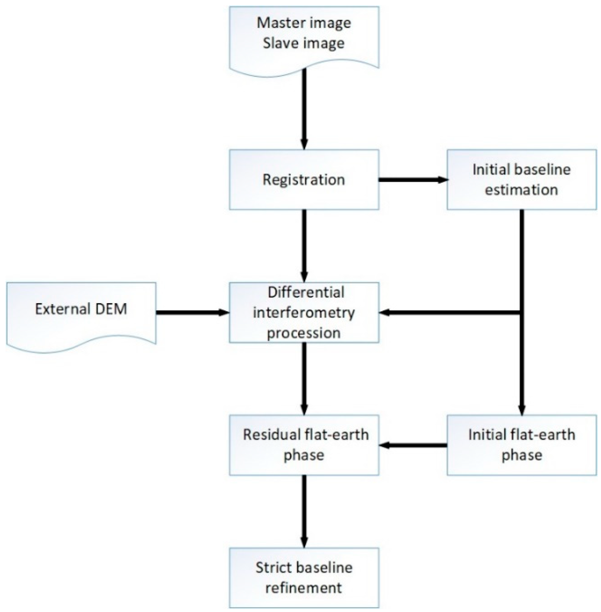
As we can see from Section 3.1, SAR interferometric baseline refinement can be strictly performed as long as the flat-earth phase ${\varphi }_{flat,unw}$ is accurately obtained. There are two steps for obtaining an accurate flat-earth phase. First, calculate the initial baseline using the orbital state vector, as well as the corresponding flat-earth phase ${\varphi }_{flat,init}$. Due to the inaccurate baseline, ${\varphi }_{flat,init}$ is not equal to ${\varphi }_{flat,unw}$. Furthermore, process differential interferometry using the initial baseline combined with external DEM and unwrap the interferogram. Then, calculate the flat-earth phase residue with planar polynomial fitting, which will be verified in the experiment part. Add ${\varphi }_{flat,res}$ and ${\varphi }_{flat,init}$ to make ${\varphi }_{flat,unw}$. Therefore, a detailed flow of the proposed algorithm for baseline refinement is as follows:

• Register master and slave images, and estimate the initial baseline using the orbital state vector to get $B_{c,0}^0$, $B_{n,0}^0$, ${\alpha }_c^0$, and ${\alpha }_n^0$;
• Process differential interferometry of SAR data using initial baseline results, and calculate flat-earth phase ${\varphi }_{flat,res}$ from the unwrapped interferogram using planar polynomial fitting;
• Calculate flat-earth phase ${\varphi }_{flat,init}$ using initial baseline estimation and add ${\varphi }_{flat,res}$ and ${\varphi }_{flat,init}$ obtained from step 2 to make a “true” unwrapped flat-earth phase ${\varphi }_{flat,unw}$;
• Refine the interferometric baseline strictly and obtain an accurate estimation of the SAR interferometric baseline. Firstly, establish adjustment models of baseline parameters, including a functional model with ${\varphi }_{flat,unw}$ obtained from step 3 based on the method introduced in Section 3.1 and the random model. Then, calculate the model parameters according to the algorithm in Section 3.2. By expanding Equation (11) into Taylor Series to build the normal equation, simultaneously calculate the sum of weighted squared residual $SWST$. The iteration mainly exists in ridge estimation and truncated singular value decomposition (TSVD). The magnitude relationship between $x_{old}^2$ and $x_{new}^2$ resulting from the iteration above is regarded as the terminative condition of iteration. If the condition is met, end the iteration and output the accurate SAR interferometric baseline estimation.
  The specific flowchart is shown in Figure 2.

4. Experiment and Results

4.1. Synthetic Dataset Experiment

4.1.1. Polynomial Fitting of Interferometric Baseline Error

According to InSAR imaging geometry and the corresponding theoretical formulas, the error of the interferometric baseline affects not only the removal of the flat-earth phase, but also the transformation coefficient between the topographic phase and elevation, which will affect the topographic phase removal for D-InSAR and the accuracy of the finally generated DEM product for InSAR. In order to quantitatively analyze the effect of baseline error, especially the impact on the removal of the flat-earth phase, an experiment is carried out by a random synthetic dataset. At first, synthesize 50 sets of baselines with different lengths in the range of 50–2500 m, and then simulate the DEM is. Calculate the “true” flat-earth phase and topographic phase combined with the parameters of the ALOS PALSAR imaging system. Following this, add 100 groups of random errors with 0 means to each set of baseline parameters (the standard deviations of the added baseline errors are ${\sigma }_{B_{c,0}}=1.3$ m, ${\sigma }_{B_{n,0}}=0.9$ m, ${\sigma }_{{\alpha }_c}=3$ mm·s⁻¹, and ${\sigma }_{{\alpha }_n}=2$ mm·s⁻¹, respectively, and eliminate the baseline error more than two times the standard deviation), and use the baseline with errors to simulate the flat-earth phase and topographic phase. Next, calculate the difference value between the flat-earth phase simulated with baseline error and that without baseline error, and conduct the same operation for the topographic phase. Then, we get the residuals of the flat-earth phase ${\varphi }_{flat,res}$ and residuals of the topographic phase ${\varphi }_{top,res}$ caused by the baseline error. Since we only add the baseline error into the simulation experiment, the resulting residuals of the flat-earth phase and topographic phase will only be related to the baseline estimation, independent of other errors (e.g., DEM errors), so the sum of residuals is also called the baseline error phase. Next, we can analyze the baseline error by polynomial fitting, for which we can use the quadratic polynomial model, that is,

$${\varphi }_{fit}=a_0+a_{1}x+a_{2}y+a_{3}xy+a_4{x}^2+a_5{y}^2,$$

(26)

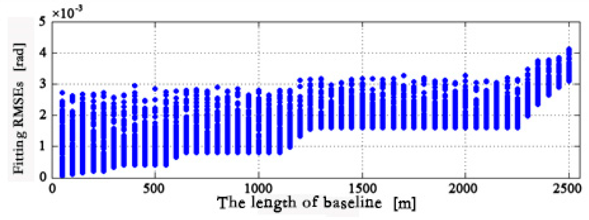
where ${\varphi }_{fit}$ is the baseline error phase obtained by fitting; x and y are normalized coordinates in the range and azimuth, respectively; and ${\alpha }_i\left(i=0,1,\cdots ,5\right)$ is the unknown model parameters; (see bibliography of [22] for more details). Then, we differ ${\varphi }_{flat,res}$ and ${\varphi }_{fit}$ as ${\varphi }_{fit}$, and calculate the corresponding root-mean-square errors (RMSEs). In this way, we can obtain the result of quadratic polynomial fitting in 5000 groups of experiments, and the RMSEs are shown as Figure 3.

4.1.2. Baseline Refinement of Simulation Data

On the basis of the experiments in Section 4.1.1, we first added the random errors with the range of [0,16] meters to the “true” DEM. Then, we simulated the DEM and the topographic phase by 5000 groups of the above-mentioned baselines with and without errors, to obtain the interferogram with baseline errors and DEM errors, as well as the “true” interferogram without any errors. Next, we differed the “true” interferogram and the one with errors to get the initial differential interferograms. To make the experimental results more reliable, we added the decorrelation error, atmospheric delay error, and random phase noise to the initial interferogram [34], so as to generate 5000 scenes of differential interferograms.

In the experiment, we refined the baselines of 5000 scenes of interferograms using the LS method. In order to reduce the effect of random phase noise, we filtered the differential interferograms by the Goldstein filter (filtering window is 32 × 32 pixels, filtering factor $\alpha =0.5,$ and the size of overlap is 14 pixels) [35], and then unwrapped the filtered interferograms by minimum cost flow (MCF) [13] to obtain the differential interferograms. In the experiment, we estimated the baselines accurately with 50 × 50 points selected uniformly in each interferogram. For baseline refinement based on the flat-earth phase, in this study, we firstly retrieved the flat-earth phase ${\varphi }_{flat,res}$ by quadratic polynomials from the unwrapped differential interferogram and calculated ${\varphi }_{flat,init}$ with initial baselines, the sum of which is the “true” unwrapped flat-earth phase ${\varphi }_{flat,unw}$. Then, we refined the baselines based on the theories presented in Section 3.1 and Section 3.2. Similarly, the accurate baseline estimation by the LS method is also based on the above-mentioned 50 × 50 GCPs of which the elevations are without DEM errors.

4.2. Real Dataset Experiment

On August 7, 2010, a sudden rainstorm occurred in the northeast mountains in Zhouqu County in Gansu Province, causing extraordinarily serious mountain torrents and geological disasters. The resulting debris flow was about 5 km long and 300 m wide, the flow region of which was wiped out. Two scenes of PALSAR data covering the interest area were used to verify the interferometric baseline refinement method mentioned above, and the details are provided in

Table 1. Parameters of the PALSAR data used in the Zhouqu region.

Parameter	Master_Image	Slave_Image
Data	2010-06-23	2010-08-08
Track	23,508	24,179
Frame	660	660
Imaging Model	FBD	FBD
Perpendicular Baseline B⊥	440 m

Note: B_⊥.: the perpendicular baseline; FBD: Fine-Beam Double polarization.

. Given the lack of GCPs in such an area, the conventional LS method cannot be applied here. Therefore, the new method proposed in this paper, refining the baselines without GCP, is a better choice.

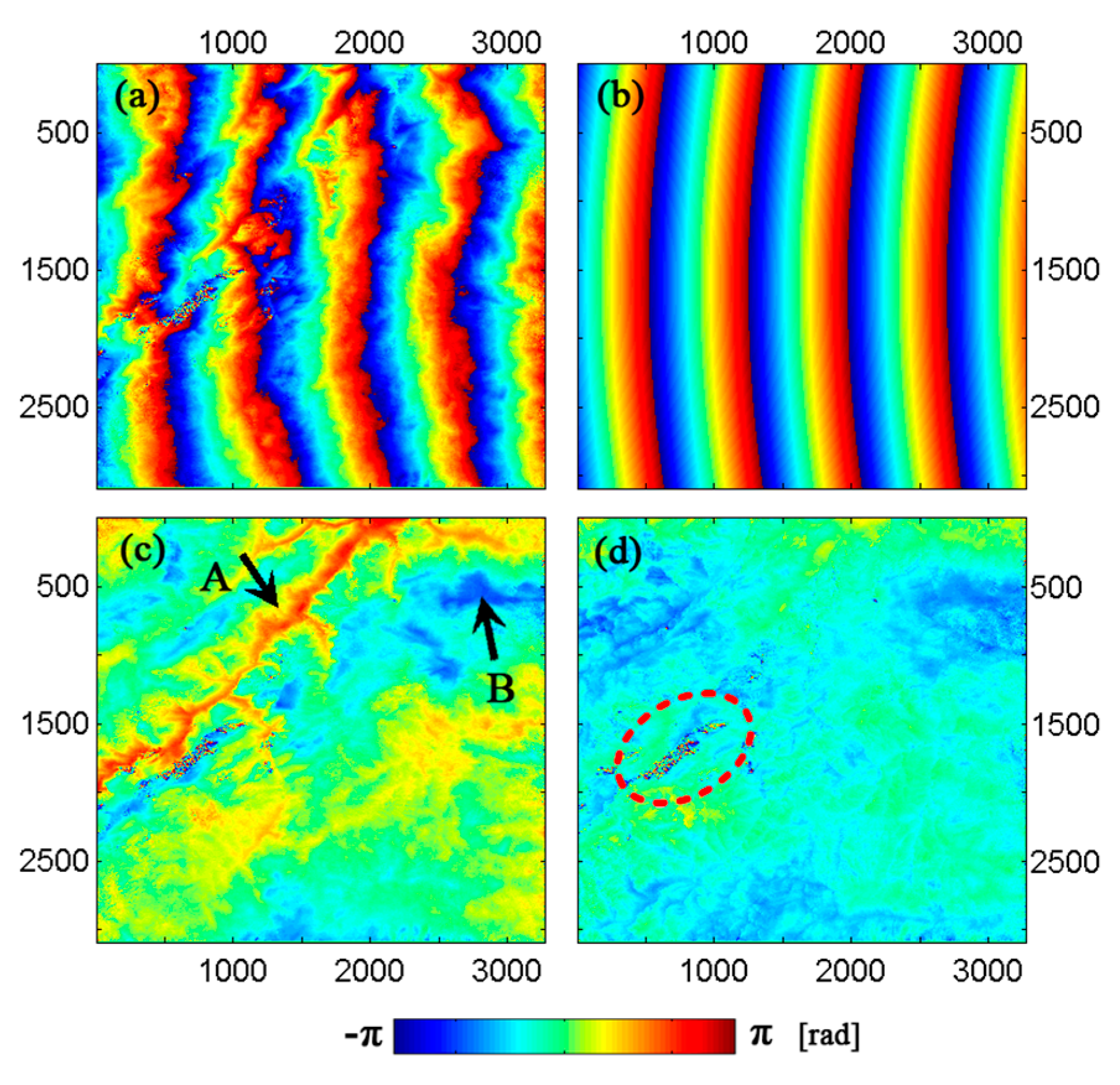
GAMMA software [13] was used for data preprocessing. Firstly, we transformed the Raw data into single look complex images (SLC) with the modular SAR processor (MSP) module. Then, we generated an interferogram from SLCs according to differential InSAR procedures, estimated the initial baselines based on orbit state vectors, and removed the flat-earth phase with SRTM DEM [36,37] by using the interferometric SAR processor (ISP) module. The generated interferogram is shown as Figure 4a.

5. Discussion

5.1. The Discussion about the Results of Synthetic Dataset

5.1.1. The Discussion about Polynomial Fitting

As we can see from Figure 3, if the length of the baseline is less than 2500 m, the quadratic polynomial can fit the flat-earth phase residuals well due to the baseline errors, of which the RMSEs are as small as a 10⁻³ rad magnitude. With the increase of the lengths of baselines, fitting RMSEs will gradually converge to a small range. Even the RMSEs in such cases will present an increasing trend, the trend is still small and the maximum RMSE is less than 4.2 × 10⁻³ rad. Therefore, it is proved that the quadratic polynomial can fit the flat-earth phase residual ${\varphi }_{flat,res}$ well, where the fitting error is too small to be counted. In this way, we can accurately obtain the flat-earth phase by using the quadratic polynomial to fit its residuals with the initial baseline estimation, so that we can refine the baseline strictly based on the theories presented in Section 3.1 and Section 3.2.

5.1.2. The Discussion about Baseline Refinement

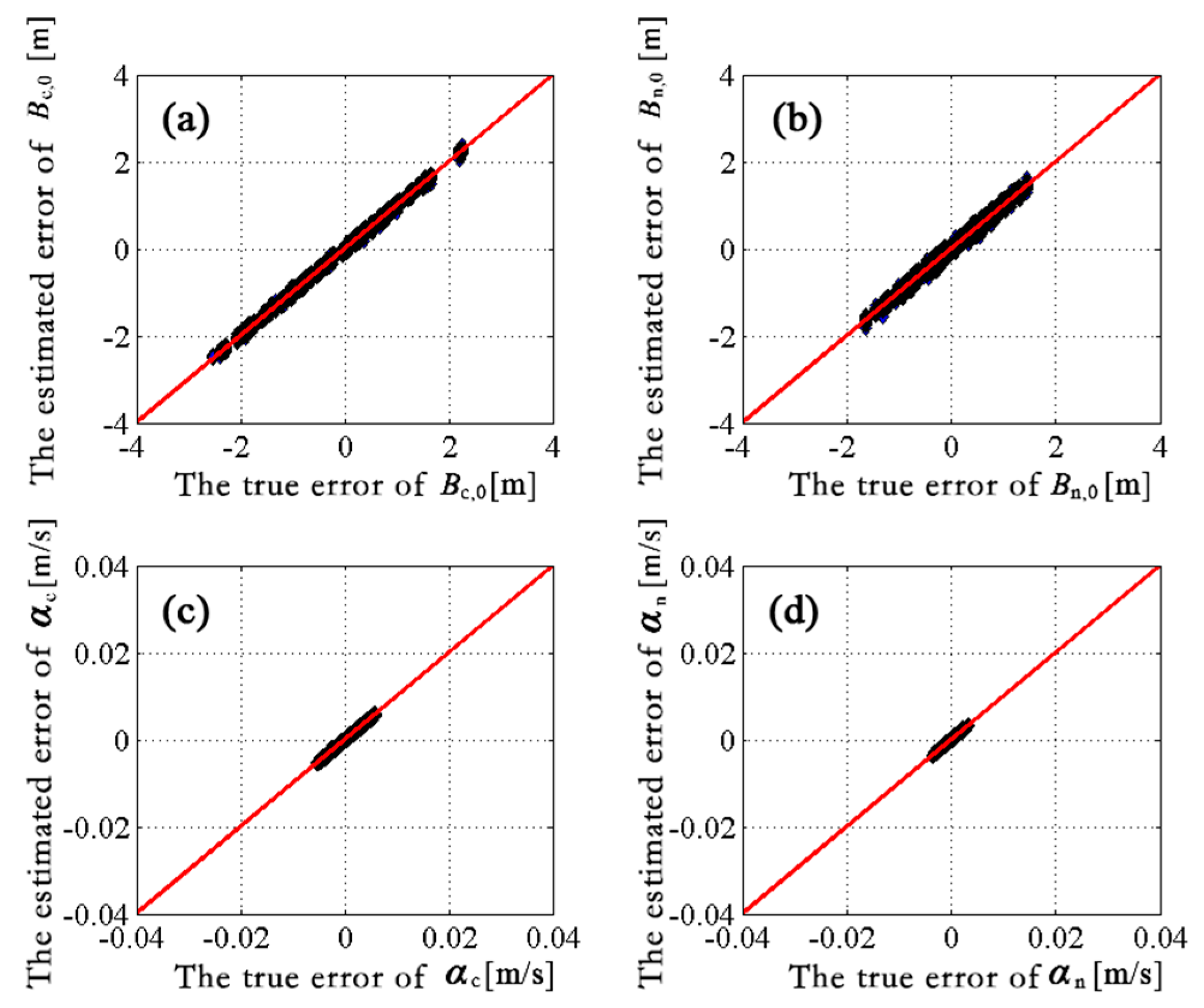
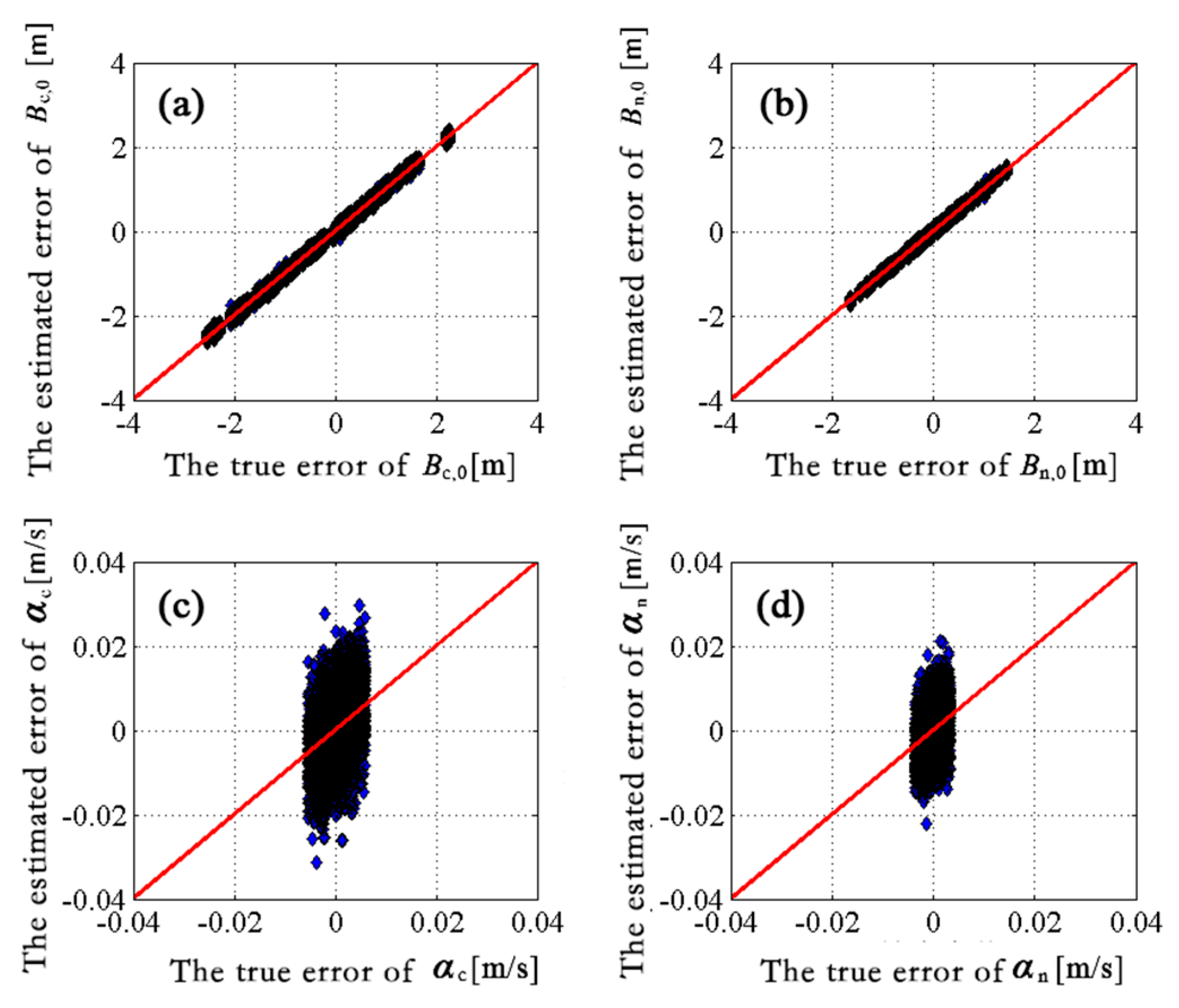
Figure 5 and Figure 6 show the comparison results of the baseline parameters for the two baseline refinement methods, respectively (by calculating the subtraction of the parameters mentioned above), from which we can see the quantitative evaluation results of the two methods. Four subgraphs (a)–(d) in the figures show the comparison results of $B_{c,0}^0$, $B_{n,0}^0$, ${\alpha }_c$, and ${\alpha }_n$, respectively. If the gaps between two kinds of errors are small, the scattered points in the figure will regress to the red (diagonal) line. By comparing the subgraphs (a) in Figure 5 and Figure 6, we can see that the baseline parameter $B_{c,0}$ obtained by our method regresses more than LS, which testifies that $B_{c,0}$ estimated by our method is more accurate. By comparing subgraphs (b), the accuracy of $B_{n,0}$ obtained by our method is a little poorer than that of LS. From the comparison between subgraphs (c) and (d) in Figure 5 and Figure 6, we can see that our method has great advantages in ${\alpha }_c$ and ${\alpha }_n$ (baseline change rate), as the estimation results almost exclusively lie on the red (diagonal) line, while large dispersion appears for the conventional LS method.

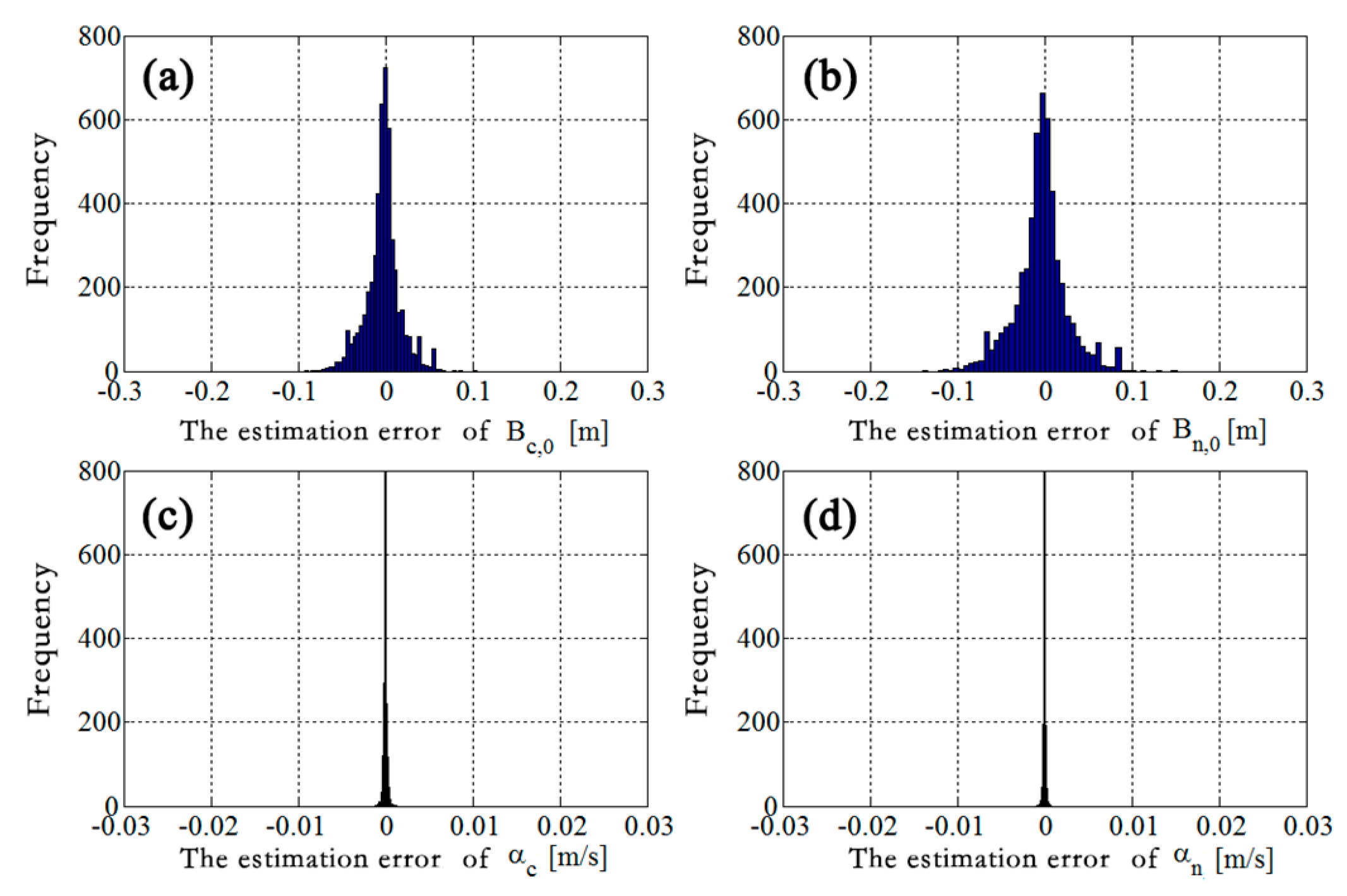
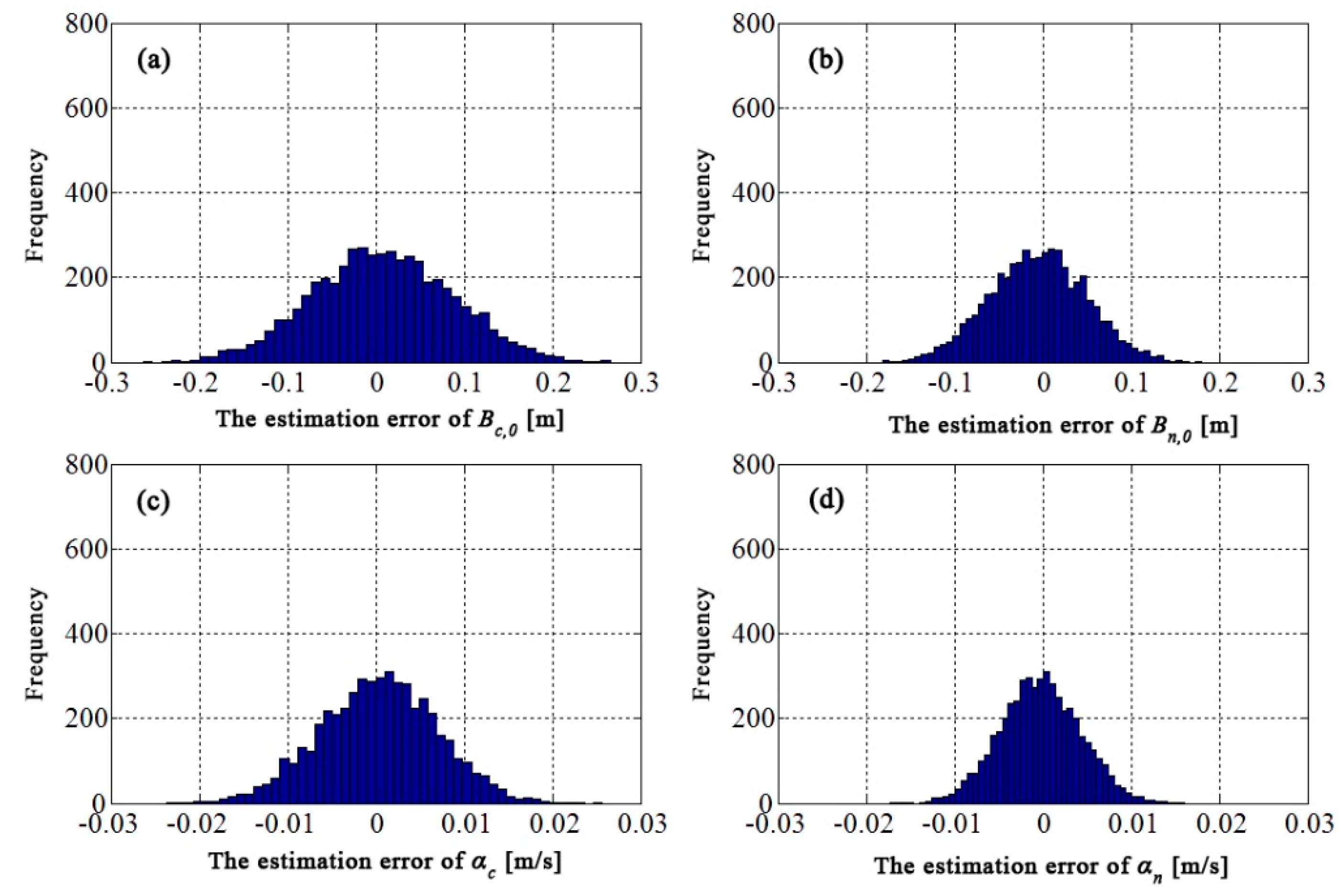
From the quantitative evaluation results, we can see that parameters $B_{c,0}$ and $B_{n,0}$ are almost the same for the two methods. For a deeper evaluation, we calculated the differences between simulated errors and calculated errors for the two methods and statistically analyzed them in histograms (see Figure 7 and Figure 8). The figures show that the estimation errors of $B_{c,0}$ and $B_{n,0}$ are more concentrated at 0, most of which are in the range of [−0.05, 0.05] m, while the errors of the LS method are more dispersed. For parameters ${\alpha }_c$ and ${\alpha }_n$, the estimations are almost all concentrated at 0 for the new method, and those for the LS method are scattered, for which quite a number of the estimation errors are greater than 10 mm/s and some errors are even greater than 20 mm/s. To conclude, the new baseline estimation method is better than the conventional LS method, especially for estimation of the baseline change rate.

For a deeper quantitative evaluation, we calculated the RMSE of the differences between simulated errors and calculated errors for the two methods, respectively. They are shown in

Table 2. Quantitative evaluation of the baseline estimation methods.

Baseline Estimation Methods	${\mathit{B}}_{\mathit{c},0}$		${\mathit{B}}_{\mathit{n},0}$		${\mathit{\alpha }}_{\mathit{c}}$		${\mathit{\alpha }}_{\mathit{n}}$
	RMSE (cm)	Percentage (<5 cm)	RMSE (cm)	Percentage (<5 cm)	RMSE (mm/s)	Percentage (<0.5 mm/s)	RMSE (mm/s)	Percentage (<0.5 mm/s)
LS Method	6.8	53.3%	4.7	71.2%	7.4	5.4%	5.1	8.2%
New Method	3.3	87.1%	4.8	75.0%	0.1	99.7%	0.1	100%

. For baseline parameter $B_{c,0}$, the accuracy of the LS method is 6.8 cm, and only 53.3% of the estimation results are less than 5 cm in 5000 groups of experiments, while the accuracy reaches 3.3 cm of the new method, which exhibits a 51.5% improvement in estimating over the LS method. In addition, 87.1% of the results are less than 5 cm, and 33.8% are higher than those of the LS method. For parameter $B_{n,0}$, it can be considered that the accuracies of the two methods are almost the same, since the differences between RMSE and the corresponding proportion are not so large. Considering baseline parameters $B_{c,0}$ and $B_{n,0}$ comprehensively, it can be found that the accuracy of $B_{n,0}$ is higher than that of $B_{c,0}$ for the LS method, while the trend for the proposed method is the opposite, but the accuracy is superior to that of the LS method. Further, the method proposed in this paper estimates baselines based on the flat-earth phase, independent of the external elevation, so the factor affected by elevation is invalid, leading to a higher accuracy.

For baseline change rates ${\alpha }_c$ and ${\alpha }_n$, the accuracies of the two methods are obviously different. The RMSEs are 7.4 and 5.1 mm/s, respectively, for the LS method, where the proportions of the error range less than 0.5 mm/s are only 5.4% and 8.2%. However, the RMSEs of the new method are 0.1 and 0.1 mm/s, respectively, and the proportions of the error range less than 0.5 mm/s reach 99.7% and 100%. With respect to a standard SAR image with a moderate resolution, the interval of the acquisition is generally around 15 s, for example, it is 14 s for PALSAR. Here, we select the acquisition time of the SAR scene center as the reference time of the baseline model, and the maximum relative time is 7 s. For the error of baseline change rate mentioned above, the maximum baseline error caused by the baseline change rate is only 0.7 mm for the new method, which is almost negligible. Conversely, the baseline errors can be up to 5.2 and 3.6 cm for the LS method. Furthermore, adding errors of $B_{c,0}$ and $B_{n,0}$ to them, we can get baseline errors of more than 0.1 m. It can be seen that the accuracy of interferometric baseline constant estimation in the C direction for the new method is obviously improved compared to the conventional LS method, the improvement of which is up to 51.5% (the ratio of reduced RMSE to the RMSE of the LS method). It proves the effectiveness of the proposed baseline estimation method.

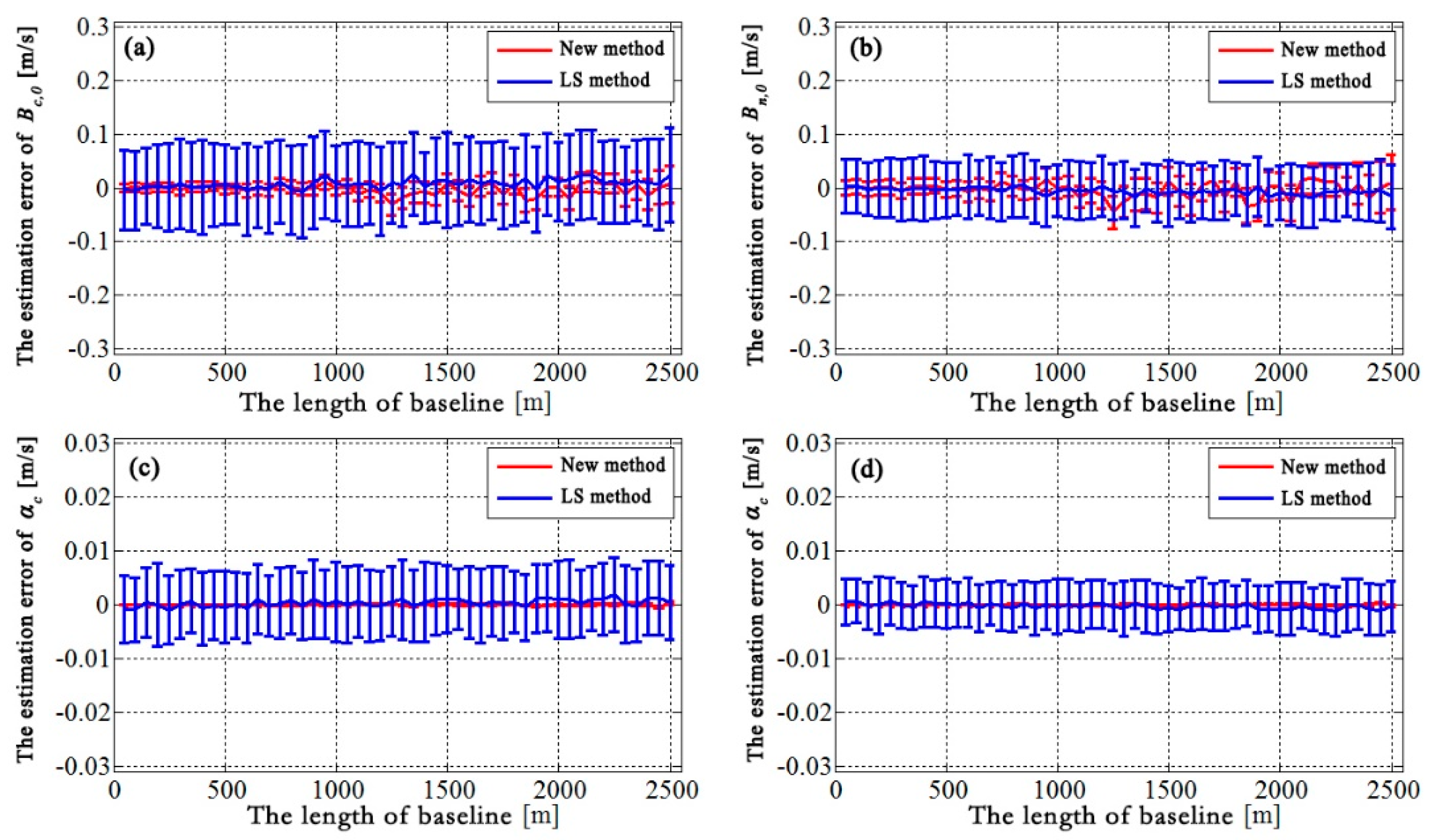
In the experiment, we selected 50 sets of baselines (the length of the baseline is in the range of 50–2500 m) with 100 experiments. Therefore, the deeper evaluation of the effect of baseline estimation due to baseline length could be analyzed from 100 repeated experiments for each set of baselines. The mean value and the standard deviation were calculated by baseline errors resulting from the repeated experiments and are shown in Figure 9. From Figure 9, the four parameters basically remain constant with the growth of baselines, and the dispersions also remain constant. This indicates that the change of baseline length does not affect the accuracy of the baseline estimations for both methods. However, the accuracy of the new method is higher than that of the LS method in the case of the same baseline length, especially for the estimation of the baseline change rate. In view of the above analysis, we can see that the new method is more effective and reliable than the LS method.

5.2. Discussion about Real Dataset Experiment

Since the area of debris flow is small (see the area within the dashed ellipse in 4d), and there is no obvious large-scale surface deformation during the interval of the two acquisitions, the fringes with longer wavelengths are caused by not completely removing the flat-earth phase caused by baseline errors, which is called the flat-earth phase residual. To obtain the flat-earth phase residual, we used MCF to unwrap the differential interferogram (Figure 4a), and used the quadratic polynomial introduced in [23] to fit the flat-earth phase residual ${\varphi }_{flat,res}$. We wrapped the flat-earth phase into the range [−π, π] to display the data conveniently (see Figure 4b). Next, we calculated ${\varphi }_{flat,init}$ with the initial baseline and added it to ${\varphi }_{flat,res}$, to get the unwrapped flat-earth phase ${\varphi }_{flat,unw}$, and then refined the baseline estimation based on the theories presented in Section 3.1 and Section 3.2. In order to visually show the accuracy of baseline refinement, we generated a new interferogram with refined baselines, shown as Figure 4d. From the figure, we can see that the flat-earth phase with longer wavelengths caused by baseline errors has been totally removed, and the main deformation area (the dashed ellipse in the figure) is well-shown. In addition, the interferogram is very flat, except for the deformation area, where there is almost no excessive fringe change rate. For a further illustration of the effect of baseline errors, the difference between Figure 4a,b is given and shown as Figure 4c. Figure 4a shows the differential interferogram with baseline errors, which will also affect the removal of the flat-earth phase and topographic phase. By subtracting Figure 4b from Figure 4a, Figure 4c obviously shows the phase residuals caused by baseline errors (e.g., arrows A/B pointing areas), while there are no such errors in the differential interferogram with refined baselines. This further demonstrates the new method is effective for baseline refinement.

6. Conclusions

Interferometric baseline estimation is a key procedure of InSAR data processing. The error of the interferometric baseline affects not only the removal of the flat-earth phase, but also the transformation coefficient between the topographic phase and elevation, which will affect the topographic phase removal for D-InSAR and the accuracy of the finally generated DEM product for InSAR. To obtain a highly accurate interferometric baseline, this paper firstly investigated the geometry of InSAR imaging, and established a rigorous relationship between the interferometric baseline and the flat-earth phase. Then, a baseline refinement method without a ground control point (GCP) was proposed, where a relevant theoretical model and resolving method were developed. Synthetic and real SAR datasets were used in the experiments, and comparisons with the conventional least-square (LS) baseline refinement method were made. The results demonstrate that the proposed method exhibits an obvious improvement over the conventional LS method, with percentages of up to 51.5% in the cross-track direction. Therefore, the proposed method is effective and advantageous.

In general, the application of the conventional LS method is limited due to the lack of available GCPs in the study area. The baseline refinement based on the LS method processes the observation (unwrapped interferometric phase) with equal weight by using the unwrapped interferometric phase and the rigorous geometric relationships of baselines when calculating the equations. Due to the errors, such as atmospheric delay error, the equal weight process will result in deviations of the results, which is obvious in the interferogram, which displays an apparent fluctuation of atmospheric error.

The interferometric baseline refinement proposed in this paper takes advantage of the unwrapped flat-earth phase and rigorous relationship of baselines, which is independent of GCP. During modeling, since the observation is the flat-earth phase without atmospheric error, the effect of atmospheric error on baseline estimation has been avoided. However, it should be noted that the flat-earth phase residual is obtained by using global polynomial fitting for the interferogram, so that the flat-earth phase may absorb some other signals, such as the deformation signal with longer wavelengths distributing globally. For this insufficiency, we can parameterize the flat-earth phase residual by using time series InSAR, where the flat-earth residual is calculated at the same time as the deformation parameters. Relevant thoughts have been studied by researchers, and will be introduced into the baseline refinement method proposed in this paper in the future to make it more general.

References

1. Zisk, S.H. A new earth-based radar technique for the measurement of lunar topography. Moon 1972, 4, 296–306. [Google Scholar] [CrossRef]
2. Gabriel, A.K.; Goldstein, R.M.; Zebker, H.A. Mapping small elevation changes over large areas: Differential radar interferometry. J. Geophys. Res. 1989, 94, 9183–9191. [Google Scholar] [CrossRef]
3. Farr, T.G.; Kobrick, M. Shuttle radar topography mission produces a wealth of data. Eos Trans. Am. Geophys. Union 2000, 81, 583–585. [Google Scholar] [CrossRef]
4. Liao, M.S.; Tang, J.; Wang, T.; Balz, T.; Zhang, L. Landslide monitoring with high-resolution sar data in the three gorges region. Sci. China-Earth Sci. 2012, 55, 590–601. [Google Scholar] [CrossRef]
5. Liu, G.X.; Jia, H.G.; Zhang, R.; Zhang, H.X.; Jia, H.L.; Yu, B.; Sang, M.Z. Exploration of subsidence estimation by persistent scatterer insar on time series of high resolution terrasar-x images. IEEE J. Sel. Top. Appl. Earth Obs. Remote Sens. 2011, 4, 159–170. [Google Scholar] [CrossRef]
6. Zhu, X.X.; Bamler, R. Very high resolution spaceborne sar tomography in urban environment. IEEE Trans. Geosci. Remote Sens. 2010, 48, 4296–4308. [Google Scholar] [CrossRef] [Green Version]
7. Qu, C.Y.; Shan, X.J.; Zhang, G.H.; Song, X.G.; Guo, L.M. Influence of interferometric baseline on measurements of seismic deformation: A case study on the 1997 mani, tibet m 7.7 earthquake. Seismol. Geol. 2012, 34, 672–683. [Google Scholar]
8. Qiu, W.N.; Tao, B.Z.; Yao, Y.B. The Theory and Method of Surveying Data Processing; Whuan University Press: Wuhan, China, 2008. [Google Scholar]
9. Wermuth, M.; Hauschild, A.; Montenbruck, O.; Jäggi, A. Terrasar-x rapid and precise orbit determination. In Proceedings of the 21st International Symposium on Space Flight Dynamics, Toulouse, France, 28 September–2 October 2009. [Google Scholar]
10. Remko, S.; Pieter, V. Precise orbit determination and gravity field improvement for the ers satellites. J. Geophys. Res. 1998, 103, 8113–8127. [Google Scholar]
11. Otten, M.; Dow, J. Envisat precise orbit determination. In Proceedings of the 2004 Envisat & Ers Symposium, Salzburg, Austria, 6–10 September 2004; pp. 6–10. [Google Scholar]
12. Nakamura, R.; Nakamura, S.; Kudo, N.; Katagiri, S. Precise orbit determination for alos. In Proceedings of the 20th International Symposium on Space Flight Dynamics, Annapolis, MD, USA, 24–28 September 2007; pp. 24–28. [Google Scholar]
13. Wegmüller, U.; Werner, C. Gamma sar processor and interferometry software. In Proceedings of the 3rd ERS Symposium, Florence, Italy, 18–21 March 1997; pp. 1686–1692. [Google Scholar]
14. Xiao, J.; Wang, C.; Li, Z.; Yang, Y. Insar baseline estimation based on co-registration offsets. Geomat. Inf. Sci. Wuhan Univ. 2010, 35, 1236–1239. [Google Scholar]
15. He, M.; He, X. An insar baseline estimation method using kalman filter. J. Remote Sens. 2008, 12, 23–27. [Google Scholar]
16. Gatelli, F.; Guamieri, A.M.; Parizzi, F.; Pasquali, P.; Prati, C.; Rocca, F. The wave number shift in sar interferometry. IEEE Trans. Geosci. Remote Sens. 1994, 32, 855–865. [Google Scholar] [CrossRef] [Green Version]
17. Li, X.; Guo, H.; Liao, J.; Wang, C.; Fan, D. Baseline estimation of interferometric sar based on fast fourier transform. Acta Geod. Cartogr. Sin. 2003, 32, 70–72. [Google Scholar]
18. Tang, X.Q. An improved baseline estimation approach based on the interferometric phases. J. Electron. Inf. Technol. 2008, 32, 2095–2099. [Google Scholar] [CrossRef]
19. Fan, H.; Deng, K.; Huang, G. Study on the methods of insar combined baseline estimation. J. Geod. Geodyn. 2009, 3, 135–140. [Google Scholar]
20. Xu, H.P.; Zhu, L.F.; Liu, X.H.; Chen, Y.F. A novel baseline estimation approach of spaceborne insar based on interferometric fringe frequency. Acta Electron. Sin. 2011, 39, 2212–2217. [Google Scholar]
21. Feng, G.C.; Ding, X.L.; Li, Z.W.; Mi, J.; Zhang, L.; Omura, M. Calibration of an insar-derived coseimic deformation map associated with the 2011 mw-9.0 tohoku-oki earthquake. IEEE Geosci. Remote Lett. 2012, 9, 302–306. [Google Scholar] [CrossRef]
22. Small, D.; Werner, C.; Nuesch, D. Baseline modelling for ers-1 sar interferometry. In Proceedings of the IGARSS‘93-IEEE International Geoscience and Remote Sensing Symposium, Tokyo, Japan, 18–21 August 1993; pp. 1204–1206. [Google Scholar]
23. Xu, B.; Li, Z.W.; Wang, Q.J.; Jiang, M.; Ding, X.L. A refined strategy for removing composite errors of sar interferogram. IEEE Geosci. Remote Sens. Lett. 2014, 11, 143–147. [Google Scholar] [CrossRef]
24. Joughin, I.; Winebrenner, D.; Fahnestock, M.; Kwok, R.; Krabill, W. Measurement of ice-sheet topography using satellite-radar interferometry. J. Glaciol. 1996, 42, 10–22. [Google Scholar] [CrossRef] [Green Version]
25. Kimura, H.; Todo, M. Baseline estimation using ground points for interferometric sar. In Proceedings of the IGARSS’97 1997 IEEE International Geoscience and Remote Sensing Symposium Proceedings, Remote Sensing—A Scientific Vision for Sustainable Development, Singapore, 3–8 August 1997; pp. 442–444. [Google Scholar]
26. Liu, G.X. Monitoring of Ground Deformations with Radar Interferometry; Surveying and Mapping Press: Beijing, China, 2006. [Google Scholar]
27. Pepe, A.; Berardino, P.; Bonano, M.; Euillades, L.D.; Lanari, R.; Sansosti, E. Sbas-based satellite orbit correction for the generation of dinsar time-series: Application to radarsat-1 data. IEEE Trans. Geosci. Remote Sens. 2011, 49, 5150–5165. [Google Scholar] [CrossRef]
28. Bahr, H.; Hanssen, R.F. Reliable estimation of orbit errors in spaceborne sar interferometry the network approach. J. Geod. 2012, 86, 1147–1164. [Google Scholar] [CrossRef] [Green Version]
29. Hoerl, A.E.; Kennard, R.W. Ridge regression: Biased estimation for nonorthogonal problems. Technometrics 1970, 12, 55–67. [Google Scholar] [CrossRef]
30. Hansen, P.C. The truncated svd as a method for regularization. BIT Numer. Math. 1987, 27, 534–553. [Google Scholar] [CrossRef]
31. Hansen, P.C. Analysis of discrete ill-posed problems by means of the l-curve. Siam Review 1992, 34, 561–580. [Google Scholar] [CrossRef]
32. Hansen, P.C.; O’Leary, D.P. The use of the l-curve in the regularization of discrete ill-posed problems. Siam J. Sci. Comput. 1993, 14, 1487–1503. [Google Scholar] [CrossRef]
33. Dai, W.; Feng, G.; Zhu, J. A method for selecting ridge parameter based on helmert variance components estimation. J Geod. Geodyn. 2006, 26, 30–33. [Google Scholar]
34. Lee, H.; Liu, J.G. Spatial decorrelation due to topography in the interferometric sar coherence imagery. In Proceedings of the IGARSS, Hamburg, Germany, 28 June–2 July 1999; pp. 485–487. [Google Scholar]
35. Goldstein, R.M.; Werner, C.L. Radar interferogram filtering for geophysical applications. Geophys. Res. Lett. 1998, 25, 4035–4038. [Google Scholar] [CrossRef] [Green Version]
36. Brown, C.G.; Sarabandi, K.; Pierce, L.E. Validation of the shuttle radar topography mission height data. IEEE Trans. Geosci. Remote Sens. 2005, 43, 1707–1715. [Google Scholar] [CrossRef]
37. Rabus, B.; Eineder, M.; Roth, A.; Bamler, R. The shuttle radar topography mission—A new class of digital elevation models acquired by spaceborne radar. ISPRS J. Photogramm. Remote Sens. 2003, 57, 241–262. [Google Scholar] [CrossRef]
Figure 1. Sketch map of interferometric synthetic aperture radar (InSAR) imaging geometry. In the figure, O ( t M ) and O ( t S ) are the coordinates of the master and slave satellites in the geocentric coordinate system, respectively; t M and t S are the respective imaging time of the master and slave images; r 1 and r 2 denote the respective slant ranges of target P in the master and slave image; and are the nominal slant ranges with respect to the ellipsoid reference surface in the master and slave acquisitions, respectively; is the tilt angle of the baseline; θ and θ 0 are the look angle and nominal look angle, respectively; B and B are the perpendicular and parallel baseline, respectively.
Remotesensing 12 00233 g001
Figure 2. Flow chart of baseline refinement.
Remotesensing 12 00233 g002
Figure 3. Root mean square error map of the flat-earth residual phase fitted with a quadratic polynomial.
Remotesensing 12 00233 g003
Figure 4. Results of the baseline refinement of Zhouqu PALSAR data. (a) Original differential interferogram; (b) flat-earth residual phase retrieved by quadratic polynomial fitting; (c) difference between subplot (a) and (b); (d) re-generated differential interferogram after baseline refinement by the proposed method.
Remotesensing 12 00233 g004
Figure 5. Comparisons of the baseline parameter errors retrieved with the baseline refinement method proposed in the paper and the genuine one, as simulated. (a) the baseline parameter B c , 0 . (b) the baseline parameter B n , 0 (c) the baseline parameter α c . (d) the baseline parameter α n .
Remotesensing 12 00233 g005
Figure 6. Comparisons of the baseline parameter errors retrieved with the conventional least-square baseline refinement method and the genuine one, as simulated. (a) the baseline parameter B c , 0 . (b) the baseline parameter B n , 0 (c) the baseline parameter α c . (d) the baseline parameter α n .
Remotesensing 12 00233 g006
Figure 7. Histograms of the baseline parameter estimation errors based on the method proposed in this paper. (a) the baseline parameter B c , 0 . (b) the baseline parameter B n , 0 (c) the baseline parameter α c . (d) the baseline parameter α n .
Remotesensing 12 00233 g007
Figure 8. Histograms of the baseline parameter estimation errors based on the conventional least-square baseline refinement method. (a) the baseline parameter B c , 0 . (b) the baseline parameter B n , 0 (c) the baseline parameter α c . (d) the baseline parameter α n .
Remotesensing 12 00233 g008
Figure 9. Statistical analysis of the baseline group, where half of the vertical bar represents the standard deviation. (a) Error B c , 0 with the baseline length variation; (b) error B n , 0 ; (c) error α c ; (d) error α n .
Remotesensing 12 00233 g009