Coastal Wetland Classification with Deep U-Net Convolutional Networks and Sentinel-2 Imagery: A Case Study at the Tien Yen Estuary of Vietnam

Abstract

The natural wetland areas in Vietnam, which are transition areas from inland and ocean, play a crucial role in minimizing coastal hazards; however, during the last two decades, about 64% of these areas have been converted from the natural wetland to the human-made wetland. It is anticipated that the conversion rate continues to increase due to economic development and urbanization. Therefore, monitoring and assessment of the wetland are essential for the coastal vulnerability assessment and geo-ecosystem management. The aim of this study is to propose and verify a new deep learning approach to interpret 9 of 19 coastal wetland types classified in the RAMSAR and MONRE systems for the Tien Yen estuary of Vietnam. Herein, a Resnet framework was integrated into the U-Net to optimize the performance of the proposed deep learning model. The Sentinel-2, ALOS-DEM, and NOAA-DEM satellite images were used as the input data, whereas the output is the predefined nine wetland types. As a result, two ResU-Net models using Adam and RMSprop optimizer functions show the accuracy higher than 85%, especially in forested intertidal wetlands, aquaculture ponds, and farm ponds. The better performance of these models was proved, compared to Random Forest and Support Vector Machine methods. After optimizing the ResU-Net models, they were also used to map the coastal wetland areas correctly in the northeastern part of Vietnam. The final model can potentially update new wetland types in the southern parts and islands in Vietnam towards wetland change monitoring in real time.

1. Introduction

Currently, about 70% of the world’s population lives in coastal estuaries and around inland freshwater bodies [1,2,3]. According to [4,5], the wetland ecosystem provides humankind with a large number of products worth USD 33,000 billion yearly. However, the world’s wetlands have disappeared 64% since the 1900s [6,7], and 87% since the 1700s [8]. Together with the decline in wetlands, according to the World Wildlife Fund (WWF)—available on https://www.worldwildlife.org/ (accessed on 7 October 2020), aquatic populations have declined by 76% between 1970 and 2010.

In Vietnam, the wetland is diverse, covering approximately 5,810,000 ha, accounting for about 8% of Asia’s entire wetland areas [9,10]. Both direct and indirect values of this ecosystem in the northeastern part of Vietnam were estimated at about USD 2063–2263 per hectare per year [11]. Currently, the wetland ecosystem along the coasts is facing threats from the population growth (about 1.32%/year), the high population density (about 276 people/km2), and the rapid urbanization (about 33% since 2010) [12]. For example, in Hai Lang commune in the northeastern part, about 1,000 hectares out of 6000 hectares of mangroves have been completely degraded over the past 15 years [13], making it one of the 12 most seriously degraded ecosystems in Vietnam due to the process of urbanization and conversion to agricultural land [14]. Although the degradation and the conversion of wetlands have been warned during the last 10 years, the assessment, inventory, and monitoring of these changes are still facing difficulties due to the lack of accessibility and technology. Therefore, it is essential to equip managers with better tools to classify and monitor wetland ecosystems at least twice a year.

Deep learning is an artificial intelligence division, in which computers learn rules based on raw data input [15,16,17]. Models may boost their output based on past results or new data sources [18]. In the last five recent years, models developed based on deep learning have provided many benefits for humans in various Earth scientific fields, such as object classification [19,20,21], identifying crop suitability areas [18], classifying coastal types [22], and predicting natural hazards [23,24]. Notably, it lets environmental managers make quick and precise decisions in real time without interference by humans [25]. A few studies applied practically deep learning technic for wetland classification, and most of them proposed this technic as a future tool for environmental management. However, it is difficult to use/update the trained models from those studies for new regions because they were trained for mixed ecosystems, instead of a particular group of ecosystems.

Before developing a deep learning model for wetland classification, it is necessary to understand the definition and types of these ecosystems. Currently, there are more than 50 definitions of wetlands in the world according to different levels and purposes [26,27]. The difference between the definitions of wetlands depends on the characteristics of the wetlands and each country’s perspective on the management of wetlands. However, most of the definitions in the world consider wetlands as a specific ecosystem, influenced by the interaction between geomorphology, hydrology, soil, and local ecology. In addition, scientists from 160 countries participated in the Convention on Wetlands (further named as RAMSAR—available on https://www.ramsar.org/ (accessed on 07 October 2020) defined wetlands as a transitional ecosystem between highlands and deep wetlands [28,29]. As a specifically defined ecosystem in the RAMSAR Convention, the wetlands are a potential ecosystem that can be completely detected and monitored at different scales based on remote sensing images and deep learning techniques.

Recently, the advanced Neural Network (NN) has been a valuable tool for machines to learn dynamic non-linear associations [15]. Therefore, this network can provide a more precise prediction than former remote sensing computing strategies such as unsupervised learning, Random Forest [30,31], pixel-based, and Support Vector Machine [32,33,34]. In the recent three years, various upgraded NN networks for standard land-cover classification were proposed, such as Convolutional Neural Network (CNN) [33,35,36], R-CNN, U-Net, and Mask-RCNN [35,37,38]. For the coastal wetland classification, these deep-learning-based models using both spatial and spectral data are considered a potential end-to-end solution to separate objects affected by water. Although these networks have been considered for the inland wetland classification [26,30,39,40,41,42], the exploration of these networks for the coastal wetland classification is still limited [43,44]. One of the main challenges in the wetland classification using deep learning models is that wetland objects are mixed with dryland objects. Consequently, the models could not separate inland cover types such as inland forests, grasslands, bare soils and urban areas with wetland and permanent water, i.e., in [43,44]. In the meanwhile, the available classification models did not follow the well-known RAMSAR wetland classification system. In other words, it is difficult to use the developed deep learning models in previous studies for further coastal wetland classification. Therefore, it is necessary to make deep learning models more applicable to the coastal wetland classification of the RAMSAR system. Accordingly, other studies can use or improve the models towards a complete model for the coastal wetland classification.

Additionally, to observe wetland types in a large area, satellite images such as MODIS, Landsat, and Sentinel-2 were commonly used [45,46,47]. Compared to the MODIS and Landsat satellite images with a low spatial resolution, the Sentinel-2, as a multi-spectral imaging mission, can systematically obtain optical imagery over both inland and coastal areas at a high spatial resolution (10 to 60 m) [47]. In this research, the authors, therefore, propose ResU-Net models for coastal wetland cover prediction based on multi-temporal Sentinel-2 data in an estuary of Quang Ninh province, Vietnam. Three research questions—relevant to wetland cover classification based on deep learning models—will clarify this study:

• What are the advantages of integrating deep learning and multi-temporal remote sensing images for monitoring coastal wetland classification?
• How do the ResU-Net34 models for coastal wetland classification improve from the benchmark methods?
• How are wetland types distributed in the northeastern part of Vietnam?

In this study, multi-temporal 4-band Sentinel-2 images integrated with digital elevation models (DEM) were used as input data of the ResU-Net models for coastal wetland-cover classification. Land covers in an estuary area of about 15x18 km were used as a mask to develop a ResU-Net model for wetland cover classification. The performance of the trained ResU-Net models will be compared with results obtained from two benchmark methods, including Random Forest (RF) and Support Vector Machine (SVM). After the best model is chosen, the new Sentinel-2 images in other times can be added to interpret wetland cover changes in the Tien Yen estuary, as well as in the whole coastal area of Quang Ninh province, Vietnam. Notably, the authors will explain in detail the wetland classification of different systems (Section 2.2) and define which coastal wetland types were improved in this study. The explanation of sample collection and model development will be shown from Section 2.3, Section 2.4 and Section 2.5). The final models will be compared with benchmark methods and discussed in Section 3 and Section 4.

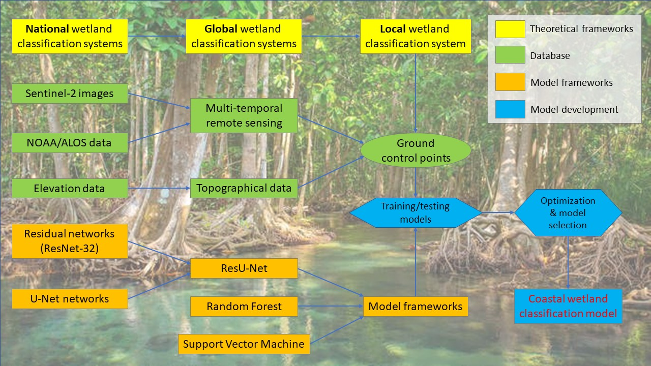
2. Materials and Methods

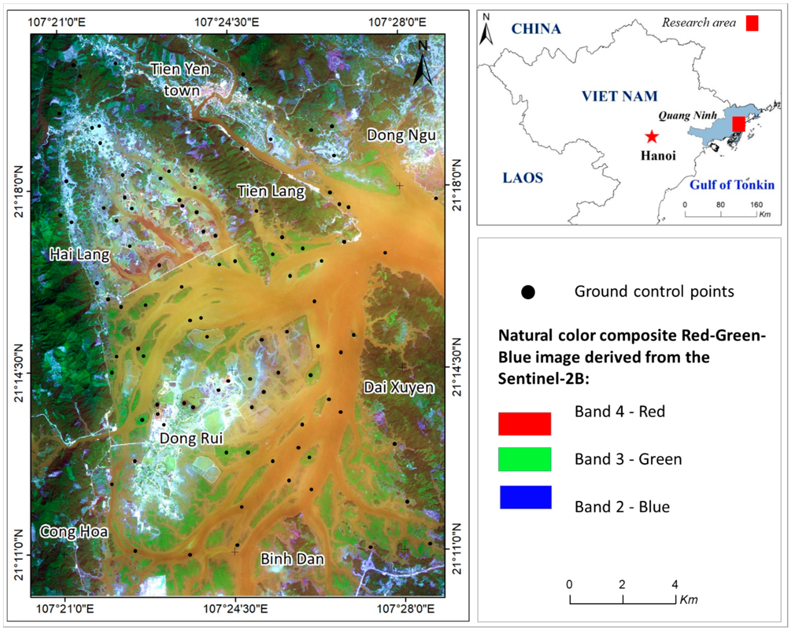
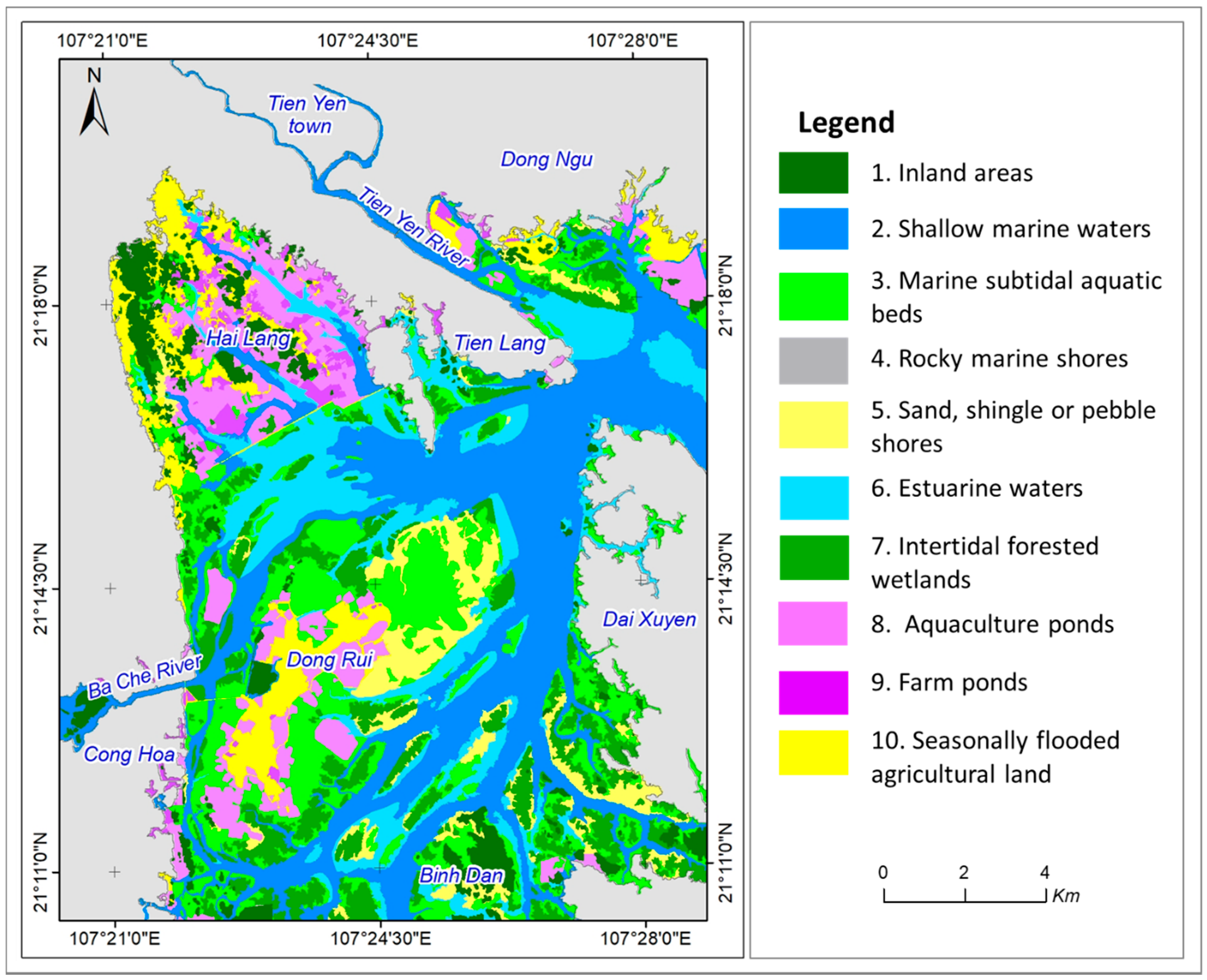
2.1. Study Area

The focus area analyzed in the topic is the wetland area of the Tien Yen estuary, which belongs to Hai Lang, Dong Ngu, Binh Dan and Dong Rui communes, Quang Ninh province of Vietnam (Figure 1). With the diurnal tide, the tidal range is about 3.5–4.0 m. The number of days with one water rise and one water down per day accounts for 85-95% of a month (i.e., over 25 days in the month). These characteristics of the tide directly affect local aquaculture. High tide amplitude and good water exchange facilitate the intake of saltwater into the ponds. However, because of high tide, the ponds must have dykes or high banks to reduce the influence of the continuous tide [48]. Accordingly, the area affected by alluvium is often used to grow two rice crops. Higher areas are often used for intercropping. Meanwhile, areas affected by seawater and tides often form saline soils, developing mangrove systems (for example, mangrove, black tiger, yellow and red).

In the dry season, the water level is lower, and the seaward flow is weaker than the rainy season. The coastal soil is affected by tidal currents, creating favorable conditions for the aquaculture of brackish water. The Tien Yen river is narrow, and the water flow from upstream areas in the rainy season often causes (1) flooding in many low-lying estuaries, (2) rapid freshening in shrimp farms, (3) increasing erosion process, leaching, (4) the destruction of dike systems, swamp farms, and sweeping away animals [49].

Regarding the land-use conversion, before 1975, Dong Rui commune mangroves account for about 3000 ha, mainly natural forests. Since 1992, Tien Yen district and Dong Rui commune have allocated 1500 hectares of mangrove land to local households. These landowners have made investments and converted mangrove land into shrimp farming ponds. However, this conversion has not brought about the expected results of the people [50]. Since 2000, the government of Dong Rui commune has made adjustments in policies and has called for a number of investment projects of the governmental and non-governmental organizations to restore and replant mangroves that have been destroyed. Especially since 2005, Dong Rui has promoted the model of community forest management, assigning specific forest areas to each village planting, tending, protecting, and exploiting, so people’s awareness of mangroves values has been raised, no one is cutting down the mangroves anymore, but they are actively protecting the forests [48]. Especially from 2012 to date, Dong Rui commune has over 3200 hectares of forest restored, and now only 500 hectares continue to be supported for restoration. Mangrove forests cover over 57% of the commune’s total natural land area. Dong Rui is considered one of the few localities with large and good quality mangrove areas of the Northeastern part of Vietnam. However, other areas outside of the Dong Rui area are currently mostly used for aquaculture [51].

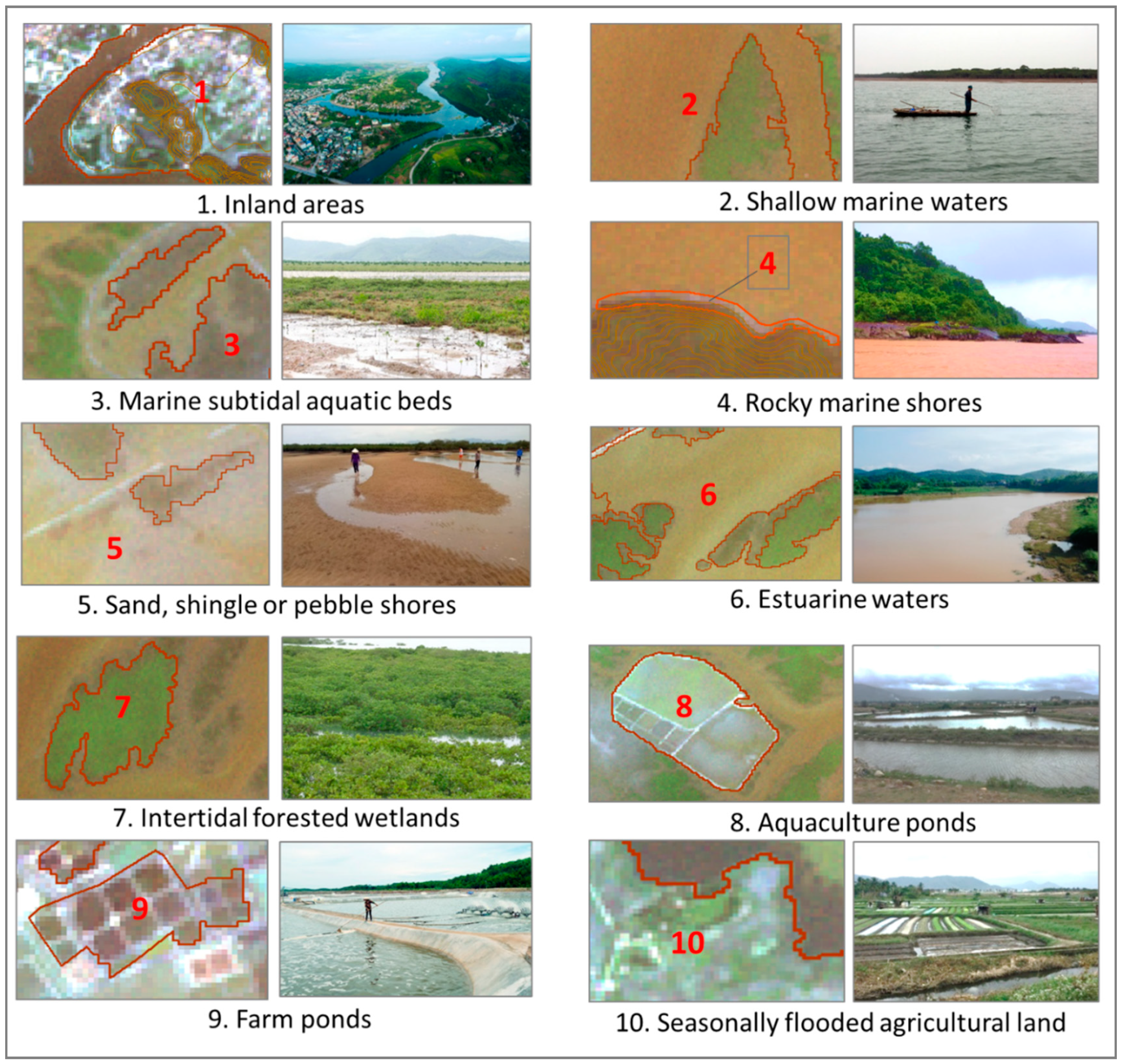
2.2. Selection of the Wetland Types for This Research

In Vietnam, the Government’s Decree No. 66/2019 / ND-CP in 2019 and the Decision No. 1093 / QD—TCMT of the Vietnam Environment Administration in 2016—the Ministry of Natural Resources and Environment (MONRE) (http://www.monre.gov.vn/English) participated in the Ramsar Convention with the concept of “Wetlands are swampy areas, peatlands, areas of regular or temporary inundation, including coastal areas and island areas, with a depth not exceeding 06 m when the tide is at the lowest tide”. Particularly, coastal wetlands include salt and brackish lands along the coast and islands where are influenced by tides [52]. In the above definitions, the wetland is generally defined as an ecological transition zone, a transitional area between terrestrial and flooded environments, or the place where soil inundation creates the development of a typical flora.

There are two main ways to classify wetlands, which are landscape- and hierarchy-based classifications [26,28,53]. A hierarchical classification system (in which the attributes used to distinguish between levels with greater differences) is superior because it allows the classification according to different levels of detail. Most classification systems have three to four categories: coastal wetlands or saltwater wetlands and inland/freshwater wetlands.

Accordingly, the study separated 19 types of coastal wetlands based on the MONRE’s classification system [54] and RAMSAR convention [29] (

Table 1. Wetland classification based on RAMSAR, MONRE, and the selection of the wetland types for the research area.

No.	Eco.	Wetland Types	RAMSAR	MONRE	Research Area
1	Natural coastal wetland	Permanent shallow marine waters	x	x	x
2		Marine subtidal aquatic beds	x	x	x
3		Coral reefs	x	x
4		Rocky marine shores	x	x	x
5		Sand, shingle or pebble shores	x	x	x
6		Estuarine waters	x	x	x
7		Intertidal mud, sand or salt flats	x	x
8		Intertidal marshes	x	x
9		Intertidal forested wetlands	x	x	x
10		Coastal brackish/saline lagoons	x	x
11		Coastal freshwater lagoons	x	x
12		Karst and other subterranean hydrological systems	x
13	Man-made wetland	Aquaculture ponds	x	x	x
14		Farm ponds	x	x	x
15		Irrigated land	x	x	x
16		Seasonally flooded agricultural land	x	x
17		Salt exploitation sites	x	x
18		Canals and drainage channels, ditches	x	x
19		Karst and other subterranean hydrological systems	x

). Among them, there are 12 types of natural wetlands and seven types of human activities. This classification has omitted two types of foreign waterways that are not available in Vietnam, including natural and man-made karst and other subterranean hydrological systems. This study focused on 10/19 types of wetlands in the northeastern coastal region of Vietnam. In this study, the irrigated and seasonal flooded agricultural lands are combined into one because these wetland types distributed discontinuously and heterogeneously in the fields, leading to difficulties in separating them from the satellite images. The remaining eight types, which occur mostly in southern regions and island systems, will not be covered in this study. Particularly for canals, drainage canals, small ditches (No.18) often have a narrow width, making it difficult to identify this object on remote sensing images. Therefore, this subject was not mentioned in this study. The detailed explanations for each type of wetland will be analyzed in Section 2.3.2.

2.3. Data and Sample Collection

The development of the deep learning models is developed through three main steps, including (1) zoning wetland areas; (2) input data preparation; and (3) training models. The structure of the deep learning model development for coastal wetland classification is shown in Figure 2. These contents will be explained in Section 2.3, Section 2.4 and Section 2.5. Firstly, Section 2.3 presents the methods to collect and set up training and validation data.

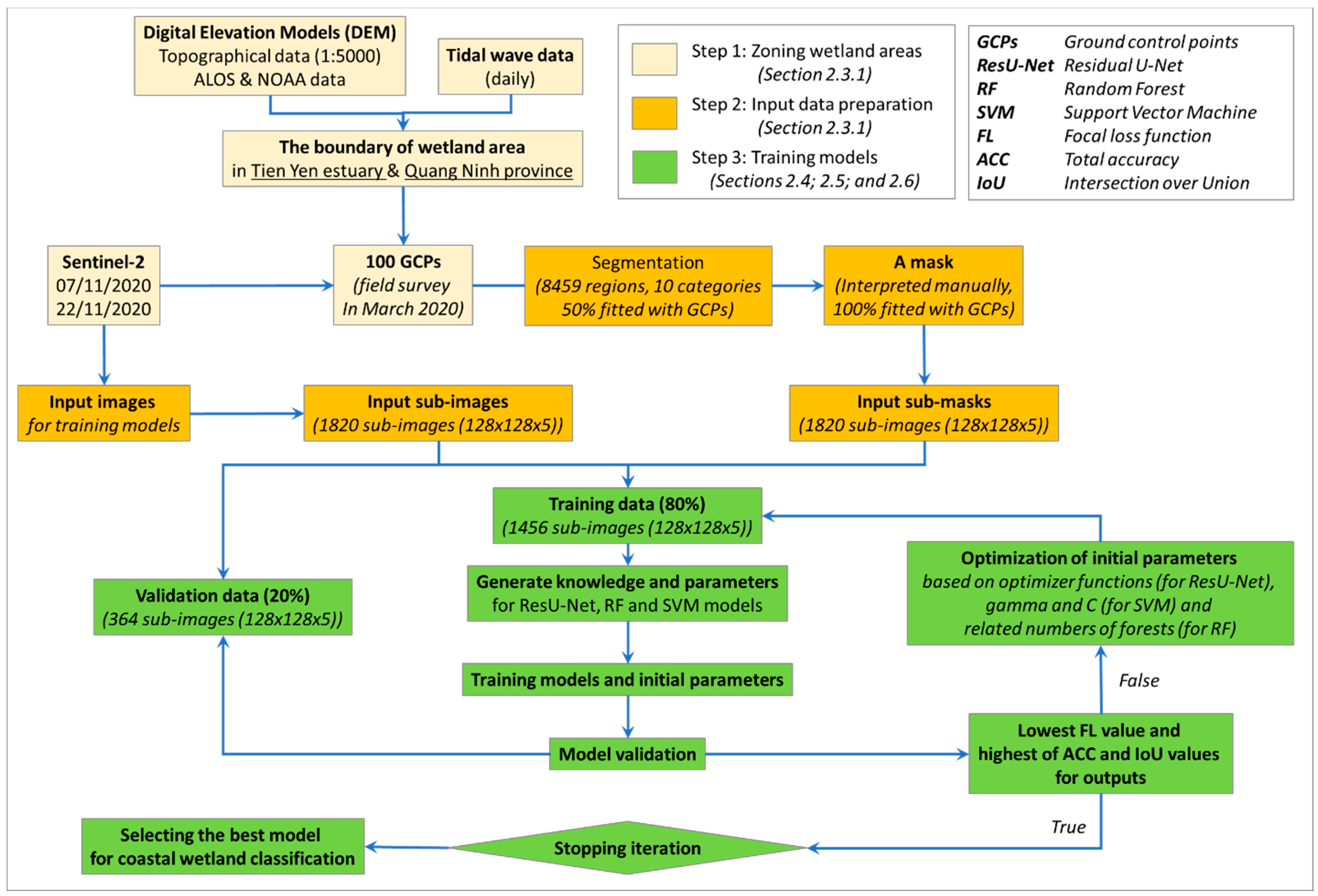
2.3.1. Input Dataset Preparation

Based on the RAMSAR definition, the coastal wetland ecosystems can be separated from coastal inland areas based on geomorphic features. The wetland areas can be identified from the areas affected by tidal to the areas at lower than −6 m of elevation. Therefore, the essential input data in this step is digital elevation models (DEM). In this study, the DEM was obtained from two sources, including topographical data at 1:5.000 of scale and the satellite data. The topographical data were used for the training process (explained in Section 2.4 and Section 2.5), whereas the DEM obtained from satellite data were used for new prediction (explained in Section 2.7). All DEM data generated in this study is not only important to separate the wetland ecosystems with the inland areas but also to detect cliffs with a slope higher than 30 degrees. The wetland areas along the cliffs are commonly “rocky marine shores” as classified in the RAMSAR system. Therefore, the slope calculated directly from the DEM data reflects the terrain surface’s steepness or degree of inclination compared to the horizontal surface [55]. The topographical data were collected only for districts surrounding the Tien Yen estuary from the Vietnam Academy of Science and Technology (VAST). The data have two continuous contour lines for every 2.5 m of elevation.

With the use of the Advanced Land Observing Satellite (ALOS) [56], 30-meters inland DEMs were downloaded from the Google Earth Engine system (https://code.earthengine.google.com/) generated by the Panchromatic Remote Sensing Instrument for Stereo Mapping (PRISM). However, the ALOS satellite data only provide the height above sea level. The ALOS DEM’s lowest value is zero; thus, at the inland border of the value ‘0’ the sea-land boundary was clearly defined. The DEM under the sea with a resolution of one arc-minute was downloaded from Global Relief Data collected by NOAA National Centers for Environmental Information (NCEI) [57]. The DEM data covered whole inland and offshore areas in the northeastern part of Vietnam and was re-projected to the WGS84 / UTM horizontal datum—48N and downscaled to a 30 meters resolution raster. Afterward, authors combined inland ALOS DEM data with the NOAA DEM ones along the boundary between sea and land (or coastline) to complete a full DEM from inland to offshore areas using ArcGIS software.

Regarding the multi-spectral satellite images, the Sentinel-2 images were chosen due to their spatial resolution of 10 meters. The use of the medium-resolution satellite image in different time is useful to separate specific narrow wetlands covered by seawater or affected by tidal such as permanent and temporal wetlands, and mangrove swamps [40,41,42]. Additionally, the Sentinel-2 images have been taken from two to three times per year in the research areas. In this study, the Sentinel-2 images taken on 07/11/2019 and 22/11/2019 were used to verify a mask for training ResU-Net models. The Sentinel-2 images were taken when the tide is 2.8 meters. As all Sentinel-2 images in 2019 and 2020 in the research area were taken at the same tidal condition, authors chose the clearer images without a cloud for training models. The satellite image interpretation from time to time can represent the current situation of each wetland type. The field works were done in March 2020 to validate wetland types in the Tien Yen estuary. The authors also used the Sentinel-2 images in three periods 2016, 2018, and 2020 for assessments of wetland changes. It will be explained in detail in Section 2.7.

2.3.2. Wetland Classification in Sentinel-2 Imagine

In the first step (zoning wetland areas) of the wetland classification, the merged DEM data were used to separate the inland areas with wetland areas in an estuary area where is strongly affected by tidal and river flow current. The tidal level in the Tien Yen estuary fluctuates from three to four meters daily, while the coastline in the topographical maps in Vietnam was identified at an average tidal level [49]. Therefore, the highest boundary of the wetland areas will be the two-meter contour line. In the topographical maps, the inland contour lines have the lowest value at 2.5 m before coming to the coastline. The distance from these lines to the coastline is lower than 10 m. Therefore, the authors chose the 2.5 m contour line as the highest boundary of the wetland areas. Additionally, according to the RAMSAR and MONRE wetland classification systems, the offshore boundary is limited at “-6” meters under the sea. It was identified easily in both the topographical maps and merged DEM data. The two objects that are separated from topographic data are “inland areas” with elevations above 2 m and “deep sea” with depths above 6m. Due to the main classified object in this study is wetland types, both “inland areas” and “and “deep sea” will be combined and called as “non-wetland” type. However, the research area in the Tien Yen estuary does not include “deep sea” type. Therefore, in the following section, the authors will only mention to “in-land” type. It is the tenth type that will be classified. In addition, nine wetland types are identified on Sentinel-2 images.

After zoning the wetland areas, the Sentinel-2 image was integrated with the field works to identify ground control points (GCPs) of one non-wetland type and nine wetland types. Firstly, two Sentinel-2 images obtained in November 2019 were segmented into polygons based on SAGA 7.6.3 software. In some regions with different tones, different shape structures are still included in the same category. Many areas of the same color, very small area sizes near each other, are assigned different object types. Therefore, visual interpretation, combined with field interpretation samples using standard GCPs, were used to reduce the degree of automatic image partition error.

The field works in March 2020 were carried out in the Tien Yen estuary, Quang Ninh province, to evaluate the indoor interpretation based on GCPs. The GCPs for image interpretation, after being analyzed and extracted from the original images, are evaluated and assessed for accuracy through field surveys. The authors built circular plots with a radius of 50 m. The authors selected randomly 10 GCPs for each inland and wetland type on the Sentinel-2 images and then verified via a field survey. The total number of standard plots for the whole study area includes 10 GCPs × 10 types = 100 GCPs. As the segmentation process that was done before the field works is an automatic partition result, the error is more than 50%, compared to the GCPs.

Figure 3 shows that the “intertidal forested wetlands” and “marine subtidal aquatic beds” types are easily identified by color and distribution structure. On the true color combination, the shallow water surface is identified among the estuary areas, easily identifiable on the image with light tones, while the “deep water surface” is easily identified on the image with darker colors and linear form. According to the coastal land use, some “intertidal forested wetlands” areas have been used for intensive aquaculture (fish farming), this wetland type can be separated into a natural type and extensive farming in mangrove forests. However, the total area of mangrove forest is too small, reducing the input samples for training models. Therefore, the authors combined them to one type as classified by the RAMSAR system.

Regarding the “farm ponds” and the “aquaculture ponds”, it is difficult to distinguish them in remote sensing images with the use of the pixel-based classification. However, these wetland types are easy to access in the fieldwork. In fact, the aquaculture ponds have been used for intensive farming without high technology, whereas the farm ponds are commonly planed for shrimp farming with high technology. The area of aquaculture ponds is commonly larger than the farm pond, but the farm ponds distribute homogeneously with each other in a large area (Figure 3). The “aquaculture ponds” can be identified with a bounded structure and light blue border and fine pattern, while the “farm ponds” includes agricultural ponds, farming ponds, small tanks (smaller than 8 ha), easily identifiable with a small plot structure, dark green color, and also surrounded by a thin bank. Therefore, the differences between these two wetland types are the area, shape, and distribution of the ponds that require object- instead of pixel-based classification.

Based on the standard interpretation of key samples, the authors conducted the interpretation of wetland objects with the same tones, structures, and shapes on Segmentation from SAGA 7.6.3. The result of the image partitioning process in step 1 created 8459 regions divided into ten categories. The visual interpretation process has normalized the boundaries of the subjects. Segmental regions with similar tones and structures are combined into one object type. Areas of different colors will be separated into other objects according to the interpretation pattern. For some objects having the same shape and color structures but different natural characteristics, we used high-resolution Google Earth images for additional interpretation. The outcomes of this step are a mask for ResU-Net development explained in the next sections.

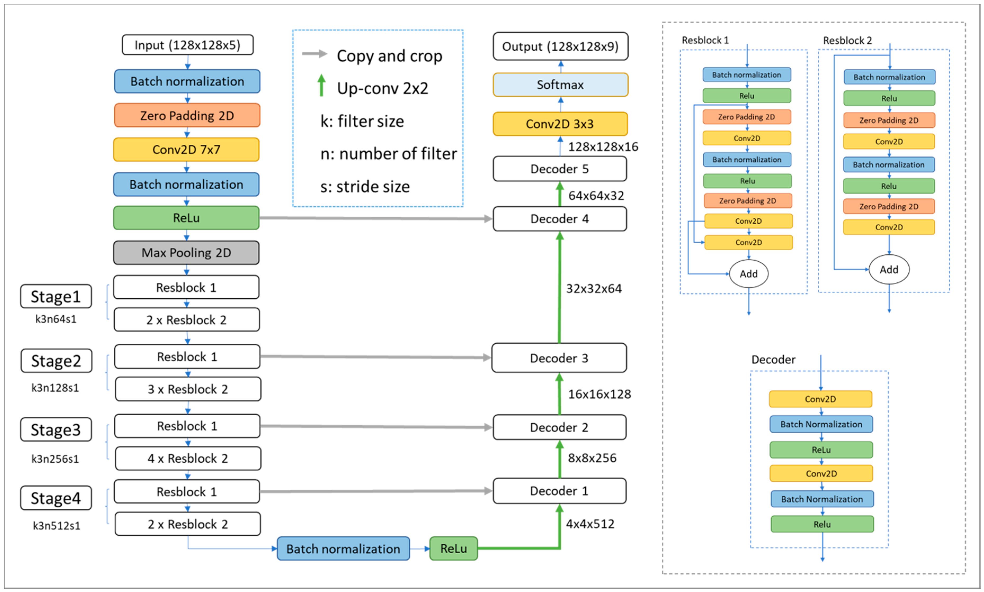
2.4. ResU-Net Architecture for Coastal Wetland Classification

According to the universal approximation theorem, a mathematical network with a single layer can represent any relations between nature and humans. However, the width of the single-layer network could be massive [58]. Hence, the geo-informatics research community needs deeper network architectures to explain non-linear correlations in nature. The increase in network depth makes the data gradients to burst and disappear [36]. Nevertheless, deeper networks (such as the 50 layers) undergo convergence degradation, leading to precision being saturated and errors staying higher than the shallower ones.

The ResU-Net (Deep Residual U-Net) is an architecture that takes advantage of deep residual neural networks with 34 layers [39,59,60] and U-Net [35,58,61]. The architecture of the proposed ResU-Net is shown in Figure 4. The ResU-Net networks integrate residual building blocks (abbreviated as ResBlock) in an encoder side of the U-Net models, whereas their decoder side remains as introduced in former U-Net architecture [62,63]. The key idea of ResNet34 is to skip the information from the initial layers in the outcomes of the ResBlocks (so-called “identity shortcut connection”. The ResBlocks propagate initial information over layers without degradation, avoiding the loss of information during the encoder process and enabling to develop a deeper neural network. It optimizes the inter-dependency between layers and reduces the computational cost by decreasing the parameters. The integration of the Resnet34 into a U-Net, therefore, allows for training of up to hundreds or even thousands of layers, while the trained network still has a high performance. The Resnet34 networks have been used in object classification, image recognition, and non-computer vision tasks [39,59]. Based on these advantages, the ResU-Net architecture is chosen as the network backbone in this study. In this section, the authors explain in detail the architecture of the ResBlock, encoder and decoder sides, as well as the development of ResU-Net models to classify coastal wetland ecosystems.

• Encoder and ResBlock architecture

Each layer of the ResU-Net transforms original data into new states based on chosen features. Five consequential types of layers were applied to build the encoder architecture include (1) INPUT Layer, (2) Batch Normalization Layer, (3) Padding layers, (4) Convolutional Layer (CONV), and (5) Pooling Layer (POOL). These five-layer types were arranged, as shown in Figure 4, to form a full ResU-Net architecture and described as follows:

• INPUT layer is added at the beginning of the ResU-Net to insert the raw pixel values of all input images to the training model. In this study, four bands (red, green, blue, and near-infrared bands), the raw Sentinel-2 images depicted in Section 2.3.1 were merged with the DEM data. Then, the input data were separated into 1820 sub-images with the dimension of 128-pixel wide, 128-pixel height, and five spectral bands.
• BATCH NORMALIZATION layer is used to standardize outcomes from the CONV layer to the same size, before a new measurement. This layer is used to optimize the distribution of the activation values during the model development, avoiding internal covariate shift problems [64]. Every layer of input data is standardized by using the mean $\left(\beta \right)$ and variance (or standard deviation - $\gamma$) parameters representing the relation between input and output batch data in the following formula:

  $$y_i=\gamma \widehat{x_i}+ \beta$$

  (1)

  where $\widehat{x_i}$ is calculated based on the mean $({\mu }_B)$ and variance $\left({\sigma }_B^2\right)$ of mini-batch M = {x1…n} as in the following formula:

  $${\mu }_M\leftarrow \frac{1}{n}{{\displaystyle \sum }}_{i=1}^n{x}_i$$

  (2)

  $${\sigma }_M^2= \frac{1}{n}{\displaystyle \sum }_{i=1}^n{\left(x_i-{\mu }_M\right)}^2$$

  (3)

  $$\widehat{x_i} \leftarrow \frac{x_{i }- {\mu }_M}{\sqrt{{\sigma }_M^2+ \epsilon }}$$

  (4)

In total, four parameters can be trained or optimized in the batch normalization layers.

• PADDING layers is a simple process to add zero-layers to input images in order to preserve information on the image corners and edges for calculation as good as the information on the image middle.
• POOLING layer is a sampled discretization process to work downscaling data by 2 × 2 spatial matrices [58]. In the ResU-Net models, the max-pooling layer was used only once before coming to the ResBlocks. In this study, the max-pooling layer is used once in the eighth layer (Appendix A). Instead of using the pooling layers to downsampling, the stride is increased from one to two
• CONV layers calculate the neural outputs using a collection of filters. The filter width and length values chosen are smaller than the input values. In this study, the chosen dimension of filters is 3 × 3. The filter slides across the images, linking input images with local regions. New pixel values are calculated with the input based on a ReLU activation functions for the filters (more detailed in Section 2.5). The ReLU functionality use max (0, x)—the threshold at zero—to preserve the images’ considerable size (128 × 128 × 5) and speed up the ResU-Net models during the convergence process [62]. In this study, the authors selected 34 CONV layers for ResU-Net construction. 64, 128, 256, and 512 filters chosen for the 34 CONV layers in the contracting direction to reduce the training and validation performance.

The ResBlock diagram integrated into the encoder side of the ResU-Net to classify the coastal wetland ecosystems is described in Figure 4. In the block diagram, the completed residual block is a combination of two layers of batch normalization, two layers of sigmoid activation function, two layers of padding, and two layers of convolution. The encoder blocks in the contracting path consist of 15 completed ResBlocks and identity shortcut connections. The identity shortcut connection is used to add the input to the output of the ResBlock. Accordingly, the input is subjected to a kernel size convolution layer of (1, 1) to increase the number of functions to the initial filter size needed. To prevent the loss of information from the initial image, a (1, 1) convolution layer was used by summing features across pixels with a larger kernel [65]. The output of whole encoder blocks is basically calculated through a “batch normalization—activation” block as a bridge to enlarge the field-of-view of filters before coming to the decoder side or an expansive path.

2.

Decoder architecture

In addition to the batch normalization and the convolution mentioned above, the expansive path uses two other layer types, including concatenate and up-sampling layers. These layers can be explained as follows:

• CONCATENATE layers are used to link information from the encoder path to the decoder path. The data is standardized from the batch normalization, and activation functions in the encoder path will be combined with up-sampled data. This process makes the prediction more accurate.
• UP-SAMPLING layers is a simple, weight-free layer that doubles the input dimensions and can be used in a generative model, following a traditional convolution layer [66]. Up-sampling is applied to recover the size of the segmentation map on the decoding path with a value of 2.

Five up-sampling blocks were generated to reduce the depth of sub-images from 512 to 256, 128, 64, 32, and 16. Each up-sampling block is designed by five-layer types, respectively, from up-sampling, concatenate, convolution, 2× batch normalization, and convolutional layers. The width and height of the sub-images in the encoder path during the concatenate processes equal to those in the decoder path. The up-sampling steps convert prediction values from the ResBlocks back to the wetland-type values.

The first convolutional layer uses a filter with a dimension of 7 × 7 to remain the information from input data, whereas the rest of the convolutional layers use a filter with the dimension of 3 × 3 in the analysis process. The number of parameters of the convolutional layers is calculated as follows:

$$P_{Conv2D}= \left(H\times W\times D\right)\times N_{Filter}$$

(5)

where ‘H’ is the height the previous filter, ‘W’ is the width of the previous filter, ‘D’ is the number of filters in the previous layer and ‘$N_{Filter}$’ is the number of filters. For instance, the second convolutional layer has (3 × 3 × 64) × 64 = 36,864 parameters.

Due to the batch normalization generate four parameters for each convolutional layer, the number of parameters in the batch normalization layer is calculated as follows:

$$P_{batch}=4\times D_i$$

(6)

whereas, $D_i$ is the depth of the input convolutional layer. For instance, the first batch normalization layer has 4 × 64 = 256 parameters. The final convolutional layer’s output is a vector with nine values, corresponding to nine wetland types. Based on 199 layers (1 × INPUT, 1 × POOL, 48 × Convolution, 45 × Batch-Normalization, 45 × Activation, 4 × Concatenate, 16 × Add, 5 × Up-Sampling, and 34 × Padding layers), the trained ResU-Net transformed the initial pixel values in raw Sentinel-2 images to the wetland classes. Parameters are assigned to 48 convolutional and 45 Batch-Normalization layers. They can be optimized with different choices of activation and optimizer functions to improve the performance and accuracy of the ResU-Net models. It will be described in detail in Section 2.6.

During ResU-Net development, the accuracy of both the training and validation data was tested to avoid overfitting and underfitting problems [59]. The best ResU-Net is chosen if the prediction of wetland types is consistent with the labels assigned from the training and validation data in the raw data. The ResU-Net model is developed based on the Segmentation model python API in Keras framework, as an API designed for image segmentation based on Tensorflow [67]. During the model-development process, all observed parameters include total accuracy and separated accuracy and loss functions of test and validation data. The ResU-Net training cycle is limited to 200 loops (epochs), but if the coefficient on the testing data set converges, the cycle can be halted if all accuracy values do not change after 20 epochs.

2.5. Alternative Options to Develop Resu-Net Models

According to the ResU-Net architecture for the wetland classification, two types of functions, including loss function and optimizer methods, can be modified to optimize the model. These functions provide optimal parameters for filters in batch-normalization and convolutional layers. The final loss function and optimizer method for the model development is chosen based on the accuracy/loss values achieved.

2.5.1. Loss Functions

The loss function represents the performance of the trained models to predict new input data. Due to the number of samples for nine wetland objects is not balance in the training and validation dataset, two types of loss functions were chosen in this study are (1) dice loss/F1 score and (2) focal loss to train ResU-Net models, instead of using traditional Multi-Class Classification Loss Functions as used by [68,69]. It reduces the imbalance of training datasets between objects, especially with the inland-area types that take a large coastal area in input data. With traditional cross-entropy loss, the loss from the negative samples dominate the overall loss and then optimize the models to predict negative samples and ignore the negative ones during the training process [67,68,70]. The focal loss that is proposed by [71] can identify this problem and optimize the models to classify the positive ones correctly. This loss function considers the loss in a global sense rather than considering it in a micro one. Therefore, it is more useful for image-level prediction than other cross-entropy loss [72]. Accordingly, the focal loss function (FL) to estimate the loss between input Sentinel-2 image (S) and the respective ground truth (G) is calculated as Formula (7). Additionally, the authors added the dice loss proposed by [73] as a function to calculate the loss at both local and global scales with high accuracy. This function that is used to estimate the overlap value between the input and mask data can be calculated by Formula (8).

$$FL = -\frac{1}{A}{{\displaystyle \sum }}_{a=1}^A{{\displaystyle \sum }}_{b=1}^B{G}_{ab}\alpha {\left(1-S_{ab}\right)}^{\gamma }ln\left(S_{ab}\right)$$

(7)

where B is assigned of 10 as the number of the wetland types, A is the number of observations in whole input data, $\alpha$ and $\gamma$ are weighting factors fluctuate from [0,5].

$$DC=\frac{2{{\displaystyle \sum }}_b^B{S}_b{G}_b}{{{\displaystyle \sum }}_b^B{S}_b^2+{{\displaystyle \sum }}_b^B{G}_b^2}$$

(8)

Based on the advantages of both focal and dice loss functions, they will be merged into one value. In this study, two other accuracy values will be calculated, including total accuracy and Intersection over Union (IoU), as the following formulas:

$$ACC= \frac{2TP}{2TP+FP+FN}$$

(9)

$$IoU= \frac{TP}{TP+FP+FN}$$

(10)

where TP is the true positive value, FP is the false positive value, and FN false negative value between prediction and ground truth. The trained model that has the lowest values of all loss functions will be the best model for classifying new wetland regions.

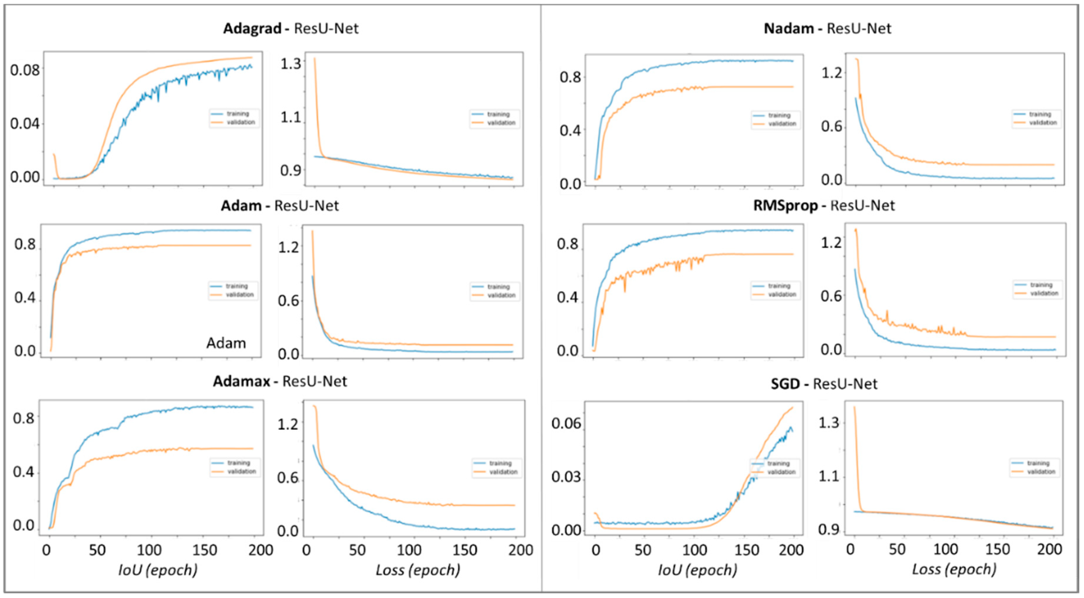
2.5.2. Optimizer Methods

Optimization approaches are widely used to build neural networks based on a stochastic gradient descent algorithm to reduce cost functions. This approach to change weights in the negative gradient direction improves the accuracy of qualified neural networks and minimizes the loss. The errors of the trained models (or the loss function) were calculated during the optimization cycles. One epoch is a period of data moving forward and backward through the ResU-Net models [74], and the update weights after each epoch is required to reduce the loss value for the next evaluation. Seven optimization algorithms were sequentially modified in this study include Adam (Adaptive Moment Estimation), Adagrad (Adaptive Gradient Algorithm), Adamax, RMSProp (Root Mean Square Propagation), SGD (Stochastic Gradient Descent algorithm), and Nadam (Nesterov-accelerated Adaptive Moment Estimation) during the ResU-Net development process.

Table 2. The seven optimization algorithms to train parameters of the ResU-Net architecture for the wetland classification, adapted from [66,67,74,75,76].

Formula	Optimizer Method	Algorithms
11	Adam	${\theta }_{t+1}={\theta }_t-\frac{\mathsf{ᵑ}}{\sqrt{{\widehat{v}}_t}+\in }{\widehat{m}}_t$
12	Adamax	${\theta }_{t+1}={\theta }_t-\frac{\mathsf{ᵑ}}{u_t}{\widehat{m}}_t$
13	Adagrad	${\theta }_{t+1}={\theta }_t-\frac{\mathsf{ᵑ}}{\sqrt{G_t+\in }}{g}_t$
14	Nadam	${\theta }_{t+1}={\theta }_t-\frac{\mathsf{ᵑ}}{\sqrt{{\widehat{v}}_t}+\in }\left({\beta }_1{\widehat{m}}_t+\frac{\left(1-{\beta }_1\right)g_t}{1-{\beta }_1^t}\right)$
15	RMSprop	$E{[g^2]}_t=0.9E{\left[g^2\right]}_{t-1}+0.1g_t^2$ and ${\theta }_{t+1}={\theta }_t-\frac{\mathsf{ᵑ}}{\sqrt{E{\left[g\right]}^2{}_t+\in }}{g}_t$
16	SGD	${\theta }_{t+1}={\theta }_t-{\eta }_t.{▽}_{\theta }Q\left({\theta }_t;x^{\left(i\right)};y^{\left(i\right)}\right)$
where $\theta$ is parameter value; $\mathsf{ᵑ}$ is the learning rates; t is time step; $\in$ = 10-8; ${\mathrm{g}}_{\mathrm{t}}$ is the gradient; E[g]—moving average of squared gradients; m, v are estimates of first and second moments; $u_t$—the max operation; $\beta$—moving average parameter (good default value—0.9); $\eta$—step size.

presents an overview of the above optimization algorithms. All in all, the best optimizer approach would produce the highest accuracy and lowest function values.

2.6. Model Comparison

In this section, the prediction results of six ResU-Net models using six optimization algorithms (so-called as Adam-ResU-Net, Adamax-ResU-Net, Adagrad-ResU-Net, Nadam-ResU-Net, RMSprop-ResU-Net, and SGD-ResU-Net) are compared with results from two benchmark models, including RF and SVM. A total of 1146 random points were chosen in the Tien Yen estuary. The wetland types interpreted from eight models and the mask were assigned to these 1146 points. The interpretation results from eight models were compared with the original information from the mask to check the performance of each trained model. Two evaluation values chosen are overall accuracy (ACC) and the kappa coefficient values. The best model will achieve the highest ACC and kappa values (presented in Section 3.2). Two benchmark models were set up in Python as follows:

2.6.1. Random Forest (RF)

In 2001, RF was proposed as a non-parametric machine learning ensemble by [77]. A forest that includes a large amount of decision trees was generated automatically and randomly, and the final stage is made by majority voting [78]. The training dataset was separated, 80% dataset were assigned as a bootstrap sample for each decision tree, and 20% dataset were assigned for validation as out of bag samples to evaluate the RF model independently. To increase the homogeneous subsets, at each node, RF chooses a subset of variables randomly and tests them to group the training data [32]. Therefore, the decision trees in the forest were varied, avoiding overfitting problems [79]. The number of trees, the number of variables, and also the number of training data are changeable parameters. Once the forest is grown, it can be used for new prediction and classification. In this study, the number of tree and variables were tested with 10, 100, 500, and 1000. Lastly, the highest accuracy was achieved with 100 trees.

2.6.2. Support Vector Machine (SVM)

The SVM is a supervised algorithm in machine learning that has been used in both classification and regression [80]. In the classification purpose, the SVM models create a hyperplane or plane to separate categories by wide gaps [78,81]. The hyperplane based on the SVM model was generated in two-dimensional space to divide the data into two categories [82]. As in this study, the training data was also set up as in the RF model. The data is converted to the corresponding multi-dimensional space data, and the plane was generated to divide data into categories [83]. In order to optimize the SVM models, two parameters were searched and optimized, including the “gamma” as a kernel coefficient and the “C” value as a penalty parameter of the error term. The increase of the gamma value can make the plane smother, and the training dataset fitted to the SVM models. Even if the error is minimized, it can create over-fitting problems. Therefore, the SVM model’s performance is affected by alternative kernel functions such as linear, polynomial, sigmoid, and radial basis (RBF) functions [84]. The “C” value limits the number of training data in the SVM development. Hence, the values “gamma” and “C” were tested to achieve the highest OA and kappa values. In this study, the optimal “gamma” value at 0.25 and “C” value at 100 were selected.

2.7. Application of Trained Resu-Net Models for New Coastal Wetland Classification

Once the final ResU-Net model was chosen, the most important function of the deep learning models is to predict the distribution of the wetland types and their changes from new Sentinel-2 images. In this study, authors downloaded the Sentinel-2 images along the coastline of the northeastern part of Vietnam since 2015. The wetland areas were prepared, as explained in detail in Section 2.3. Upon inputting these new images into the trained ResU-Net, the model accesses the trained parameters in 199 layers to convert new input images into different spatial matrices, before interpreting the final type values for each image’s pixel. Class scores will be allocated with the name of the wetland types in the FC layer. The wetland results of the final ResU-Net models will be compared with former prediction in Vietnam to assess the wetland changes in the research areas that were explained in Section 4.

3. Results

3.1. ResU-Net Model Performance

The distribution of nine wetland types and one non-wetland type in November 2019 that were obtained from visual interpretation and field interpretation samples is shown in Figure 5. It was used as the input mask for the all ResU-Net, RF, and SVM models. According to Figure 6 and

Table 3. Accuracy values for the ResU-Net models using six optimizer functions.

No.	Model	ACC Score (%)		IoU Score (%)		Loss
		Training	Validation	Training	Validation	Training	Validation
1	Adagrad	9.1	9.3	8.2	8.7	0.991	1.309
2	Adam	96.9	90.0	94.1	82.5	0.868	1.365
3	Adamax	92.9	69.4	87.1	57.5	0.959	1.361
4	Nadam	96.2	82.8	92.7	72.8	0.921	1.343
5	RMSprop	97.0	85.7	94.2	76.3	0.866	1.280
6	SGD	7.9	8.5	6.2	7.3	0.973	1.358

, the ResU-Net model using Adam optimizer has the highest accuracy with the validation data in six proposed models. Its ACC value is 90%, whereas its IoU value is 83% after 200 epochs. Two other models using the RMSprop and Nadam optimizer functions can predict the validation data with an accuracy of 85%. Accordingly, the Adagrad and SGD optimizer functions provide low accuracy values. The loss function values of the models using Adam, Adamax, RMSprop, and Nadam optimizers (so-called as Group 1) decreased from about 1.3 to 0.1, whereas those of the models using Adamax, Adagrad and SGD optimizers (so-called as Group 2) only decrease to about 0.9. Therefore, we used the models in Group 2 to predict input Sentinel-2 image and compare with the distribution of wetland ecosystems in Tien Yen district, as shown in Figure 5.

3.2. Accuracy Comparison among the Trained Models

The prediction based on the models in the Group 2 is shown in Figure 7. The coastal wetland prediction based on the RF and SVM models was shown and separate from the third group for model comparison. In general, four prediction results in Group 2 are nearly similar. The inland area, rocky marine shores, sand, shingle or pebble shores, and seasonal flooded agricultural lands were predicted correctly by all four models. It is challenging to interpret two objects: the shallow marine and estuary waters by three models using Adamax, Nadam, and RMSprop optimizers due to their mixture of sand and sea/river waters. The same situation can be found in the aquaculture and farm ponds, especially the area inside the dams of the Hai Lang district.

The performances of eight trained models (including six ResU-Net models and two benchmark models) are compared in

Table 4. The cross-validation results of eight models for the coastal wetland classification.

No.	Class	No. Sample	Aggregated Class Accuracy of Models (%)
			ResU-Net						SVM	RF
			Adagrad	SGD	Nadam	RMSprop	Adam	Adamax
1	Inland areas	156	1.3	97.4	90.9	94.2	95.5	13.6	79.2	80.5
2	Shallow marine waters	57	3.5	89.5	87.7	98.2	94.7	21.1	0.0	43.9
3	Marine subtidal aquatic beds	139	2.9	81.6	90.4	93.4	94.9	0.7	6.6	24.3
4	Rocky marine shores	271	49.8	94.4	95.1	97.7	97.0	16.5	63.5	49.6
5	Sand, shingle or pebble shores	77	3.9	92.0	94.7	97.3	94.7	9.3	20.0	24.0
6	Estuarine waters	25	0.0	72.2	77.8	88.9	88.9	11.1	0.0	77.8
7	Intertidal forested wetlands	62	48.4	85.0	78.3	90.0	95.0	1.7	28.3	48.3
8	Aquaculture ponds	196	10.7	86.9	88.0	92.1	94.8	26.2	84.3	36.6
9	Farm ponds	119	2.5	91.6	91.6	93.3	95.0	5.9	72.3	73.1
10	Seasonal flooded agricultural lands	70	22.9	61.4	67.1	62.9	58.6	57.1	78.6	68.6
Total OA (%)			18.4	84.7	85.1	88.8	89.5	12.7	50.5	46.4
Cohen’s kappa			8.5	84.4	85.2	89.1	89.6	6.9	46.7	43.2

. Due to the testing samples were chosen randomly in the research area, they can be contained in training or validation datasets. The IoU values of eight models are higher than the results depicted in Table 3. As shown in Figure 6 and Figure 7, the IoU and Kappa value of the model using the Adagrad and SGD optimizer (in Group 1) provided the lowest values, compared to other models. The interpretation results of the RF and SVM models (in Group 3) have the IoU of about 50%, whereas their kappa values only have 45% on average. However, the accuracy of the models in Group 1 and 3 is lower than four ResU-Net models using the Adam, Adamax, Nadam and RMSprop optimizers (in Group 2). Compared with the manual interpretation mask, the ResU-Net model using Adam optimizer provides the best prediction.

According to Figure 7, excepting two ResU-Net models in Group 1, the “inland areas” and “farm ponds” types can be correctly interpreted by other models. The SVM model misses all “shallow marine waters” and “estuarine waters” samples. Although the “shallow marine waters” and “estuarine waters” areas interpreted by the RF model are more accurate than those by the SVM model, the “rocky marine shores”, “aquaculture ponds” and “seasonal flooded agricultural flooded agricultural lands” interpreted by the SVM models are more accurate than those by the RF model. Although four models in the Group 3 are more accurate than two benchmark models in the Group 2 in general, the accuracy in interpreting the “seasonal flooded agricultural lands” type of these four ResU-Net models is lower than the prediction from two benchmark models, only from 60 to 67%, even with the Adam-ResU-Net model. However, the overall accuracy and kappa index of the ResU-Net model using Adam optimizer reaches about 90%. As a result, the ResU-Net model using Adam optimizer is used to predict new wetland types for the next interpretation.

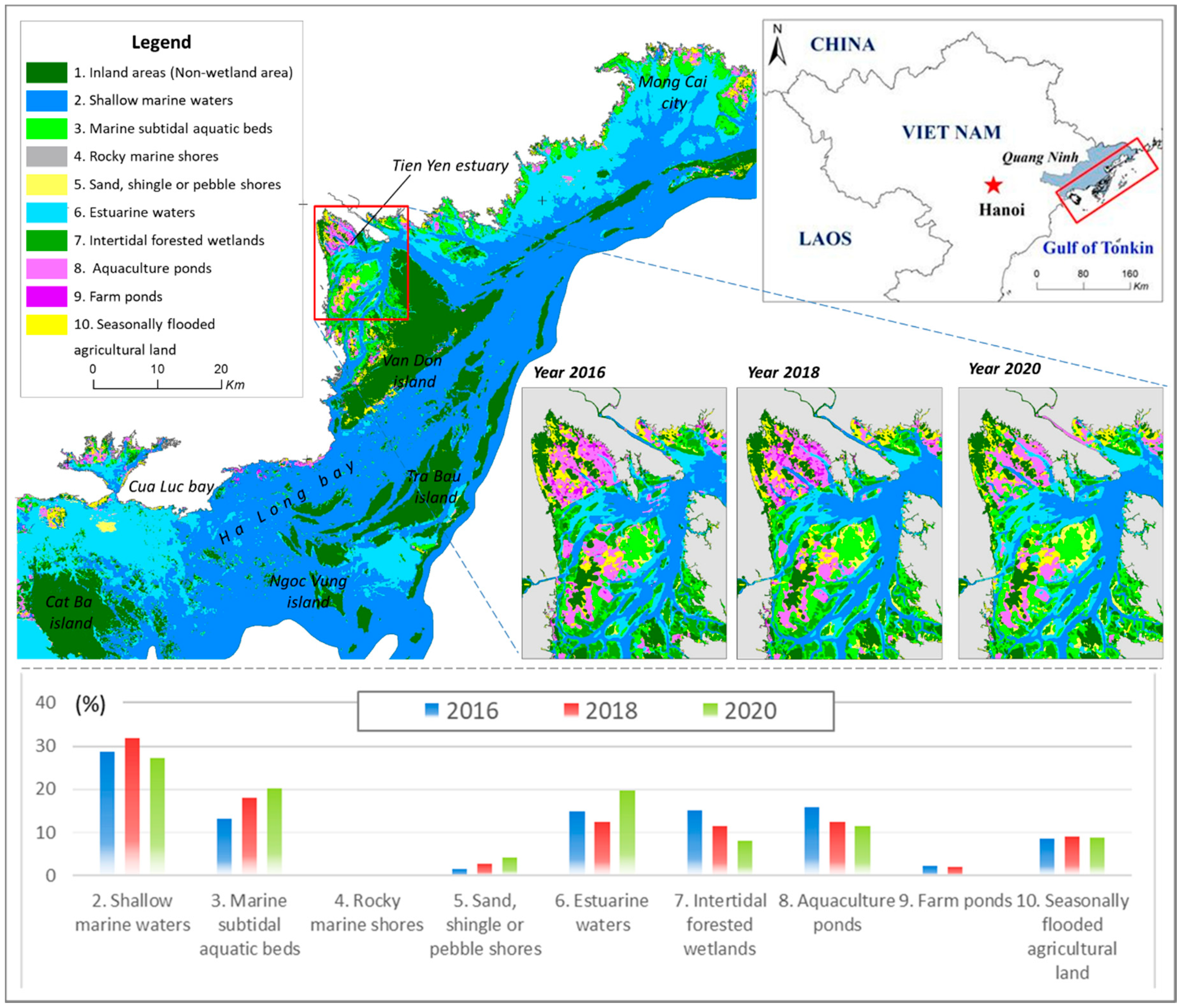
3.3. Wetland Cover Changes in Tien Yen Estuary

Based on the trained ResU-Net model using Adam optimizer, the distribution of the wetland types in the northeastern part of Vietnam was mapped in Figure 8. Its area was bordered from the depth of minus 6 meters to a tidal area of two meters. The wetland ecosystems distribute mainly in the Cua Luc bay, Tien Yen estuary and coastal area of Mong Cai city. The “marine subtidal aquatic beds” and “intertidal forested wetlands” types have enlarged in the northern part, whereas the area of the human-made wetland types such as the “aquaculture ponds” and “farm ponds” in the southern part of the area are larger than the northern parts. The area on islands was combined to “inland areas”. The “rocky marine shores” area distributes narrow around cliffs and islands such as Van Don, Cat Ba, and Tra Bau islands.

Additionally, Figure 8 also shows the areal percentage changes of wetland types in the Tien Yen estuary area in 2016, 2018, and 2020. The area of the “shallow marine waters” and the “estuary waters” are inversely proportional change. The area of shallow waters was narrowed from 29% of the area in 2016 to 27% in 2020, while the estuarine area was expanded from 15% in 2016 to 20% in 2020. It shows that the natural activity of the river to transport alluvium materials to the sea is getting stronger after the recent four years. Sand and mud were accumulated to form small islands, sandbanks, and tidal flats. The area of farm ponds and aquaculture ponds has been narrowed, from 16% in 2016 to 11% in 2020. According to the interviews in 2020, the aquaculture production is reduced significantly due to urbanization in the wetland area of the Quang Ninh province. It led to the land-use conversion from wetland to new urban. In 4 years, local economic development and uncontrolled population rate are increasing in the research area have led to a sharp decrease of mangrove area up to 50% of the area. Therefore, the program to afforest and protect mangrove ecosystems has been interested in some coastal communes of Tien Yen River by the district committee. It is reflected through the increase in planted forest area by over 20% and aquatic ecosystems by over 50% after four years. The area of the “rocky marine shores” and “seasonally flooded agricultural land” is stable, respectively, with 210,000 m² and 440,000 m².

4. Discussion

4.1. Comparison with Formal Networks/Frameworks

Compared to the wetland classification systems of RAMSAR and MONRE, this study focuses on nine coastal wetland ecosystems in the dynamic estuary in the northeastern part of Vietnam (Figure 8). Although the wetland classification models were developed in some former studies [26,40,41,43,53], the classification models for the inland and coastal wetland ecosystem should be separated to provide suitable tools for different land managers. Most of the former studies only focused on the method or models to identify wetland in technical ways instead of on explaining how their outcomes have met the standard wetland classification systems and how to practically apply the trained models for land management [40,44]. As an example, the rocky marine shores, as a specific ecosystem in the RAMSAR classification system, were identified based on the trained ResU-Net models in this study. However, they were not attended by many former studies. This ecosystem covers a narrow area with a slight slope nearby cliffs. Therefore, it is difficult to identify the rocky marine shores in Landsat or SPOT satellite images.

Additionally, the use of remote sensing data was optimized in this study, especially with the integration between Sentinel-2, ALOS, and NOAA satellite data. Adapted from the former studies, the authors used DEM as important data to extract wetland areas. The trained models can use both the DEM developed from topographical maps or from the ALOS and NOAA data. However, the DEM generated from the topographical maps can provide more accurate data than satellite images, especially the areas under the sea level. The trained model using the high-quality Sentinel-2 satellite images (without cloud cover) collected two to three times per year, can be used effectively to monitor wetland use/cover changes, instead of waiting for land use maps that have been generated every five years in many countries. Especially, the coastal wetland ecosystems in Vietnam are commonly affected by about five storm events annually. The identification of wetland changes potentially provides different information related to the quantitative changes in beneficial values of these ecosystems to coastal people, particularly with the northeastern part of Vietnam that were analyzed in this study.

4.2. Improvement of Land Cover Classification

While traditional satellite image interpretation methods require many real samples to generate a wetland cover map in a particular time and region, the final trained ResU-Net models can be used to interpret wetland types from new satellite images in any coastal area and in any time. Eleven wetland types that can be classified quickly based on the trained model and the satellite data were taken from 19 types shown in the RAMSAR and MONRE classification systems [29,54]. It is a benefit for further studies to update new samples from other areas where the other eight wetland ecosystems are developed. Notably, further studies can take more “coral reefs” samples from islands where have clear seawater and warm water temperature (20–32 °C), or coastal lagoons and salt exploration areas in the middle part of Vietnam which are strongly affected by wave action [48]. As an advantage to using deep learning models, the developers can update new samples in the trained model to make a better model. The new models do not only predict the wetland ecosystem type more accurately, but they also can identify more types if they learn correct samples. However, some specific human-made wetland types such as canals, ditches, and drainage channels in karst regions mentioned in the RAMSAR and MONRE classification systems cannot be identified in the medium-resolution satellite images. The wide of these objects is commonly lower than 10 meters. In this study, we merged these types with some nearby flooded and irrigated lands to collect the high enough number of samples. For these specific human-made wetland types, it is necessary to use high-resolution images integrated with field works to identify them correctly.

Both high or low tidal levels can affect the input samples. If the satellite images are taken at low tide, all wetland types can be identified in dry conditions. If the images are taken at high tide, the tidal flats are flooded, the results from the prediction models might show the same type of shallow wetland type. Therefore, it is important to check the tidal level when the satellite images were taken for further studies. More samples can be collected when the tidal is low in the research area to make the interpretation models become more accurate.

The ResU-Net development for coastal wetland classification requires the cost- and time-consuming dedication of scientists. In this study, the authors used a CPU Intel(R) Xeon(R) CPU @ 2.6GHz CPU with 16GB RAM and GPU NVIDIA GeForce GTX1070. The average time per epoch to train a ResU-Net model is more than 22 s. Meanwhile, the average time to train the RF and SVM models is from 45 to 60 s for each model. Although the time to train a ResU-Net model is long, the trained model can be updated from the new data. Different optimization approaches such as evolutionary or swarm intelligence algorithms may also be used for future work instead of using six optimizers to boost the ResU-Net models. It will be a possible method for the training of new information from new multi-spectral satellite image data for the qualified ResU-Net models. The supercomputer is an alternative option to rapidly classify the wetland types, especially with the use of high-resolution data.

5. Conclusions

Based on the integration of a ResU-Net34 model with the U-Net models to classify wetland ecosystem types in the northeastern part of Vietnam, the individual research questions mentioned in the introduction section are answered as follows:

• What are the advantages of integrating deep learning and multi-temporal remote sensing images for monitoring wetland classification? The completed deep learning models can be used to interpret new satellite images in any coastal area and at any time, especially in hard-to-access areas among reefs and rocky marine shores. The use of deep learning models can help coastal managers to monitor the dynamic ecosystems annually in the wetlands that have been commonly done every five years by ecologists.
• How do the ResU-Net34 models for coastal wetland classification improve from the benchmark methods? The geomorphological and land cover characteristics of nine wetland ecosystem types were recorded during the training process of ResU-Net models with an accuracy of 83% and loss function value of 1.4 based on the use of the Adam optimizer. The best-trained ResU-Net model was used to successfully classify the wetland types in the Tien Yen estuary for four years. It can potentially be used to classify whole Vietnamese coastal wetlands in the future.
• How are wetland types distributed in the northeastern part of Vietnam? Nine wetland types distributed mainly in three regions, including the Cai Lan bay, Tien Yen estuary, and the coastal area of Mong Cai city. Due to the effect of rivers, the estuary and shallow marine waters have significant fluctuation. The area of the aquaculture pools and mangrove area has been narrowed, while the marine subtidal aquatic beds have been expanded.

References

1. Dugan, P.J. Wetland Conservation: A Review of Current Issues and Action; IUCN: Gland, Switzerland, 1990. [Google Scholar]
2. Paalvast, P.; Velde, G. Van Der Ocean & Coastal Management Long term anthropogenic changes and ecosystem service consequences in the northern part of the complex Rhine-Meuse estuarine system. Ocean Coast. Manag. 2014, 92, 50–64. [Google Scholar] [CrossRef] [Green Version]
3. Mahoney, P.C.; Bishop, M.J. Assessing risk of estuarine ecosystem collapse. Ocean Coast. Manag. 2017, 140, 46–58. [Google Scholar] [CrossRef]
4. Li, T.; Gao, X. Ecosystem services valuation of Lakeside Wetland park beside Chaohu Lake in China. Water (Switzerland) 2016, 8, 301. [Google Scholar] [CrossRef]
5. Russi, D.; ten Brink, P.; Farmer, A.; Bandura, T.; Coates, D.; Dorster, J.; Kumar, R.; Davidson, N. The Economics of Ecosystems and Biodiversity for Water and Wetlands; IEEP London and Brussels: London, UK, 2012. [Google Scholar]
6. RAMSA. Wetlands: A global disappearing act. Available online: https://www.ramsar.org/document/ramsar-fact-sheet-3-wetlands-a-global-disappearing-act (accessed on 8 October 2020).
7. Davidson, N.C. How much wetland has the world lost? Long-term and recent trends in global wetland area. Mar. Freshw. Res. 2014, 65, 934–941. [Google Scholar] [CrossRef]
8. CBD. Wetlands and Ecosystem Services; United Nations, 2015. [Google Scholar]
9. Duc, L.D. Wetland Reserves in Vietnam (In Vietnamese); Centre for.; Agricultural Publishing House: Hanoi, Vietnam, 1993. [Google Scholar]
10. Buckton, S.T.; Cu, N.; Quynh, H.Q.; Tu, N.D. The Conservation of Key Wetland Sites in the Mekong Delta; BirdLife International Vietnam Porgramme: Hanoi, Vietnam, 1989. [Google Scholar]
11. Hawkins, S.; To, P.X.; Phuong, P.X.; Thuy, P.T.; Tu, N.D.; Cuong, C.V.; Brown, S.; Dart, P.; Robertson, S.; Vu, N.; et al. Roots in the Water: Legal Frameworks for Mangrove PES in Vietnam; Katoomba Group’s Legal Initiative Country Study Series: Washington, DC, USA, 2010. [Google Scholar]
12. McDonough, S.; Gallardo, W.; Berg, H.; Trai, N.V.; Yen, N.Q. Wetland ecosystem service values and shrimp aquaculture relationships in Can Gio, Vietnam. Ecol. Indic. 2014, 46, 201–213. [Google Scholar] [CrossRef]
13. Pedersen, A.; Nguyen, H.T. The Conservation of Key Coastal Wetland Sites in the Red River Delta; Hanoi BirdLife International Programme; Eames, J.C., Ed.; BirdLife International: Hanoi, Vietnam, 1996. [Google Scholar]
14. Naganuma, K. Environmental planning of Quang Ninh province to 2020 vision to 2030. Quang Ninh Prov. People’s Comm. 2014. [Google Scholar]
15. Lary, D.J.; Alavi, A.H.; Gandomi, A.H.; Walker, A.L. Machine learning in geosciences and remote sensing. Geosci. Front. 2016, 7, 3–10. [Google Scholar] [CrossRef] [Green Version]
16. Balakrishnan, N.; Muthukumarasamy, G. Crop Production - Ensemble Machine Learning Model for Prediction. Int. J. Comput. Sci. Softw. Eng. 2016, 5, 148–153. [Google Scholar]
17. Ma, X.; Deng, X.; Qi, L.; Jiang, Y.; Li, H.; Wang, Y.; Xing, X. Fully convolutional network for rice seedling and weed image segmentation at the seedling stage in paddy fields. PLoS ONE 2019, 14, 1–13. [Google Scholar] [CrossRef]
18. Dang, K.B.; Burkhard, B.; Windhorst, W.; Müller, F. Application of a hybrid neural-fuzzy inference system for mapping crop suitability areas and predicting rice yields. Environ. Model. Softw. 2019, 114, 166–180. [Google Scholar] [CrossRef]
19. Shi, Q.; Li, W.; Tao, R.; Sun, X.; Gao, L. Ship Classification Based on Multifeature Ensemble with Convolutional Neural Network. Remote Sens. 2019, 11, 419. [Google Scholar] [CrossRef] [Green Version]
20. Gray, P.C.; Fleishman, A.B.; Klein, D.J.; McKown, M.W.; Bézy, V.S.; Lohmann, K.J.; Johnston, D.W. A convolutional neural network for detecting sea turtles in drone imagery. Methods Ecol. Evol. 2019, 10, 345–355. [Google Scholar] [CrossRef]
21. Guo, Q.; Jin, S.; Li, M.; Yang, Q.; Xu, K.; Ju, Y.; Zhang, J.; Xuan, J.; Liu, J.; Su, Y.; et al. Application of deep learning in ecological resource research: Theories, methods, and challenges. Sci. China Earth Sci. 2020, 2172. [Google Scholar] [CrossRef]
22. Dang, K.B.; Dang, V.B.; Bui, Q.T.; Nguyen, V.V.; Pham, T.P.N.; Ngo, V.L. A Convolutional Neural Network for Coastal Classification Based on ALOS and NOAA Satellite Data. IEEE Access 2020, 8, 11824–11839. [Google Scholar] [CrossRef]
23. Gebrehiwot, A.; Hashemi-Beni, L.; Thompson, G.; Kordjamshidi, P.; Langan, T.E. Deep convolutional neural network for flood extent mapping using unmanned aerial vehicles data. Sensors (Switzerland) 2019, 19, 1486. [Google Scholar] [CrossRef] [Green Version]
24. Feng, P.; Wang, B.; Liu, D.L.; Yu, Q. Machine learning-based integration of remotely-sensed drought factors can improve the estimation of agricultural drought in South-Eastern Australia. Agric. Syst. 2019, 173, 303–316. [Google Scholar] [CrossRef]
25. Dang, K.B.; Windhorst, W.; Burkhard, B.; Müller, F. A Bayesian Belief Network – Based approach to link ecosystem functions with rice provisioning ecosystem services. Ecol. Indic. 2018. [Google Scholar] [CrossRef]
26. Guo, M.; Li, J.; Sheng, C.; Xu, J.; Wu, L. A review of wetland remote sensing. Sensors (Switzerland) 2017, 17, 777. [Google Scholar] [CrossRef] [Green Version]
27. Mahdianpari, M.; Granger, J.E.; Mohammadimanesh, F.; Salehi, B.; Brisco, B.; Homayouni, S.; Gill, E.; Huberty, B.; Lang, M. Meta-analysis of wetland classification using remote sensing: A systematic review of a 40-year trend in North America. Remote Sens. 2020, 12, 1882. [Google Scholar] [CrossRef]
28. Ozesmi, S.L.; Bauer, M.E. Satellite remote sensing of wetlands. Wetl. Ecol. Manag. 2002, 10, 381–402. [Google Scholar] [CrossRef]
29. Davis, T.J. (Ed.) The Ramsar Convention Manual: A Guide for the Convention on Wetlands of International Importance Especially as waterfowl Habitat; Ramsar Convention Bureau: Gland, Switzerland, 1994. [Google Scholar]
30. Tian, S.; Zhang, X.; Tian, J.; Sun, Q. Random forest classification of wetland landcovers from multi-sensor data in the arid region of Xinjiang, China. Remote Sens. 2016, 8, 954. [Google Scholar] [CrossRef] [Green Version]
31. Mahdianpari, M.; Salehi, B.; Mohammadimanesh, F.; Motagh, M. Random forest wetland classification using ALOS-2 L-band, RADARSAT-2 C-band, and TerraSAR-X imagery. ISPRS J. Photogramm. Remote Sens. 2017, 130, 13–31. [Google Scholar] [CrossRef]
32. Chen, X.; Wang, T.; Liu, S.; Peng, F.; Tsunekawa, A.; Kang, W.; Guo, Z.; Feng, K. A New Application of Random Forest Algorithm to Estimate Coverage of Moss-Dominated Biological. Remote Sens. 2019, 11, 18. [Google Scholar]
33. Liu, T.; Abd-Elrahman, A. Deep convolutional neural network training enrichment using multi-view object-based analysis of Unmanned Aerial systems imagery for wetlands classification. ISPRS J. Photogramm. Remote Sens. 2018, 139, 154–170. [Google Scholar] [CrossRef]
34. Alizadeh, M.R.; Nikoo, M.R. A fusion-based methodology for meteorological drought estimation using remote sensing data. Remote Sens. Environ. 2018, 211, 229–247. [Google Scholar] [CrossRef]
35. Garg, L.; Shukla, P.; Singh, S.K.; Bajpai, V.; Yadav, U. Land use land cover classification from satellite imagery using mUnet: A modified UNET architecture. In Proceedings of the 14th International Joint Conference on Computer Vision, Imaging and Computer Graphics Theory and Applications (VISIGRAPP 2019), Prague, Czech Republic, 25–27 February 2019; Volume 4, pp. 359–365. [Google Scholar]
36. Albawi, S.; Mohammed, T.A.; Al-Zawi, S. Understanding of a convolutional neural network. In Proceedings of the 2017 International Conference on Engineering and Technology (ICET), Antalya, Turkey, 21–23 August 2017; pp. 1–6. [Google Scholar] [CrossRef]
37. Stoian, A.; Poulain, V.; Inglada, J.; Poughon, V.; Derksen, D. Land cover maps production with high resolution satellite image time series and convolutional neural networks: Adaptations and limits for operational systems. Remote Sens. 2019, 11, 1986. [Google Scholar] [CrossRef] [Green Version]
38. Liu, B.; Li, Y.; Li, G.; Liu, A. A spectral feature based convolutional neural network for classification of sea surface oil spill. ISPRS Int. J. Geo-Information 2019, 8, 160. [Google Scholar] [CrossRef] [Green Version]
39. Pouliot, D.; Latifovic, R.; Pasher, J.; Duffe, J. Assessment of convolution neural networks for wetland mapping with landsat in the central Canadian boreal forest region. Remote Sens. 2019, 11, 772. [Google Scholar] [CrossRef] [Green Version]
40. DeLancey, E.R.; Simms, J.F.; Mahdianpari, M.; Brisco, B.; Mahoney, C.; Kariyeva, J. Comparing deep learning and shallow learning for large-scalewetland classification in Alberta, Canada. Remote Sens. 2020, 12, 2. [Google Scholar] [CrossRef] [Green Version]
41. Gordana, K.; Avdan, U. AVDAN Evaluating Sentinel-2 Red-Edge Bands for Wetland Classification. Proceedings 2019, 18, 12. [Google Scholar] [CrossRef] [Green Version]
42. Slagter, B.; Tsendbazar, N.-E.; Vollrath, A.; Reiche, J. Mapping wetland characteristics using temporally dense Sentinel-1 and Sentinel-2 data: A case study in the St. Lucia wetlands, South Africa. Int. J. Appl. Earth Obs. Geoinf. 2020, 86, 102009. [Google Scholar] [CrossRef]
43. Wang, X.; Gao, X.; Zhang, Y.; Fei, X.; Chen, Z.; Wang, J.; Zhang, Y.; Lu, X.; Zhao, H. Land-cover classification of coastal wetlands using the RF algorithm for Worldview-2 and Landsat 8 images. Remote Sens. 2019, 11, 1927. [Google Scholar] [CrossRef] [Green Version]
44. Abubakar, F.A.; Boukari, S. A Convolutional Neural Network with K-Neareast Neighbor for Image Classification. Int. J. Adv. Res. Comput. Commun. Eng. (IJARCCE) 2018, 7, 1–7. [Google Scholar] [CrossRef]
45. Bacour, C.; Baret, F.; Béal, D.; Weiss, M.; Pavageau, K. Neural network estimation of LAI, fAPAR, fCover and LAI×Cab, from top of canopy MERIS reflectance data: Principles and validation. Remote Sens. Environ. 2006, 105, 313–325. [Google Scholar] [CrossRef]
46. Zambrano, F.; Vrieling, A.; Nelson, A.; Meroni, M.; Tadesse, T. Prediction of drought-induced reduction of agricultural productivity in Chile from MODIS, rainfall estimates, and climate oscillation indices. Remote Sens. Environ. 2018, 219, 15–30. [Google Scholar] [CrossRef]
47. Feng, Q.; Yang, J.; Zhu, D.; Liu, J.; Guo, H.; Bayartungalag, B.; Li, B. Integrating multitemporal Sentinel-1/2 data for coastal land cover classification using a multibranch convolutional neural network: A case of the Yellow River Delta. Remote Sens. 2019, 11, 1006. [Google Scholar] [CrossRef] [Green Version]
48. Amaral, G.; Bushee, J.; Cordani, U.G.; KAWASHITA, K.; Reynolds, J.H.; ALMEIDA, F.F.M.D.E.; de Almeida, F.F.M.; Hasui, Y.; de Brito Neves, B.B.; Fuck, R.A.; et al. Overview of Wetlands Status in Viet Nam Following 15 Years of Ramsar Convention Implementation Table. J. Petrol. 2013, 369, 1689–1699. [Google Scholar] [CrossRef]
49. Tran, H.D.; Ta, T.T.; Tran, T.T. Importance of Tien Yen Estuary (Northern Vietnam) for early-stage Nuchequula nuchalis (Temminck & Schlegel, 1845). Chiang Mai Univ. J. Nat. Sci. 2016, 15, 67–76. [Google Scholar] [CrossRef]
50. Nguyen, T.N.; Duong, T.T.; Nguyen, A.D.; Nguyen, T.L.; Pham, T.D. Primary assessment of water quality and phytoplankton diversity in Dong Rui Wetland, Tien Yen District, Quang Ninh Province. VNU J. Sci. 2017, 33, 6. [Google Scholar]
51. Ha, N.T.T.; Koike, K.; Nhuan, M.T. Improved accuracy of chlorophyll-a concentration estimates from MODIS Imagery using a two-band ratio algorithm and geostatistics: As applied to the monitoring of eutrophication processes over Tien Yen Bay (Northern Vietnam). Remote Sens. 2013, 6, 421–442. [Google Scholar] [CrossRef] [Green Version]
52. De Groot, D.; Brander, L.; Finlayson, M. Wetland Ecosystem Services. Wetl. B. 2016, 1–11. [Google Scholar] [CrossRef]
53. He, Z.; He, D.; Mei, X.; Hu, S. Wetland classification based on a new efficient generative adversarial network and Jilin-1 satellite image. Remote Sens. 2019, 11, 2455. [Google Scholar] [CrossRef] [Green Version]
54. Hoang, V.T.; Le, D.D. Wetland Classification System in Vietnam; CRES, Viet.; Vietnam Environment Administration: Hanoi, Vietnam, 2006. [Google Scholar]
55. Stage, A.R.; Salas, C. Composition and Productivity. Soc. Am. For. 2007, 53, 486–492. [Google Scholar]
56. Ghuffar, S. DEM generation from multi satellite Planetscope imagery. Remote Sens. 2018, 10, 1462. [Google Scholar] [CrossRef] [Green Version]
57. Mussardo, G. Digital Elevation Models of the Northern Gulf Coast: Procedures, Data sources and analysis. Stat. F. Theor 2019, 53, 1689–1699. [Google Scholar] [CrossRef]
58. Diakogiannis, F.I.; Waldner, F.; Caccetta, P.; Wu, C. ResUNet-a: A deep learning framework for semantic segmentation of remotely sensed data. ISPRS J. Photogramm. Remote Sens. 2020, 162, 94–114. [Google Scholar] [CrossRef] [Green Version]
59. Perez, H.; Tah, J.H.M.; Mosavi, A. Deep learning for detecting building defects using convolutional neural networks. Sensors (Switzerland) 2019, 19, 3556. [Google Scholar] [CrossRef] [Green Version]
60. Scott, G.J.; Marcum, R.A.; Davis, C.H.; Nivin, T.W. Fusion of Deep Convolutional Neural Networks for Land Cover Classification of High-Resolution Imagery. IEEE Geosci. Remote Sens. Lett. 2017, 14, 1638–1642. [Google Scholar] [CrossRef]
61. Zhang, P.; Ke, Y.; Zhang, Z.; Wang, M.; Li, P.; Zhang, S. Urban land use and land cover classification using novel deep learning models based on high spatial resolution satellite imagery. Sensors (Switzerland) 2018, 18, 3717. [Google Scholar] [CrossRef] [Green Version]
62. Liu, Z.; Feng, R.; Wang, L.; Zhong, Y.; Cao, L. D-Resunet: Resunet and Dilated Convolution for High Resolution Satellite Imagery Road Extraction. Int. Geosci. Remote Sens. Symp. 2019, 3927–3930. [Google Scholar] [CrossRef]
63. Jakovljevic, G.; Govedarica, M.; Alvarez-Taboada, F. A deep learning model for automatic plastic mapping using unmanned aerial vehicle (UAV) data. Remote Sens. 2020, 12, 1515. [Google Scholar] [CrossRef]
64. Garcia-Pedrero, A.; Lillo-Saavedra, M.; Rodriguez-Esparragon, D.; Gonzalo-Martin, C. Deep Learning for Automatic Outlining Agricultural Parcels: Exploiting the Land Parcel Identification System. IEEE Access 2019, 7, 158223–158236. [Google Scholar] [CrossRef]
65. Zhang, C.; Sargent, I.; Pan, X.; Li, H.; Gardiner, A.; Hare, J.; Atkinson, P.M. An object-based convolutional neural network (OCNN) for urban land use classification. Remote Sens. Environ. 2018, 216, 57–70. [Google Scholar] [CrossRef] [Green Version]
66. Iglovikov, V.; Mushinskiy, S.; Osin, V. Satellite Imagery Feature Detection using Deep Convolutional Neural Network: A Kaggle Competition. Available online: https://arxiv.org/abs/1706.06169 (accessed on 8 October 2020).
67. Gulli, A.; Pal, S. Deep Learning with Keras—Implement Neural Networks with Keras on Theano and TensorFlow; Packt Publishing Ltd.: Birmingham, UK, 2017; ISBN 9781787128422. [Google Scholar]
68. Lapin, M.; Hein, M.; Schiele, B. Analysis and Optimization of Loss Functions for Multiclass, Top-k, and Multilabel Classification. Pattern Anal. Mach. Intell. 2017, 8828, 1–20. [Google Scholar] [CrossRef] [PubMed] [Green Version]
69. Li, B.; Liu, Y.; Wang, X. Gradient Harmonized Single-Stage Detector. In Proceedings of the AAAI Conference on Artificial Intelligence, Honolulu, HI, USA, 27 January–1 February 2019; Volume 33, pp. 8577–8584. [Google Scholar] [CrossRef]
70. Ahuja, K. Estimating Kullback-Leibler Divergence Using Kernel Machines. In Proceedings of the 2019 53rd Asilomar Conference on Signals, Systems, and Computers, Pacific Grove, CA, USA, 3–6 November 2019; pp. 690–696. [Google Scholar] [CrossRef] [Green Version]
71. Lin, T.Y.; Goyal, P.; Girshick, R.; He, K.; Dollar, P. Focal Loss for Dense Object Detection. IEEE Trans. Pattern Anal. Mach. Intell. 2020, 42, 318–327. [Google Scholar] [CrossRef] [Green Version]
72. Pasupa, K.; Vatathanavaro, S.; Tungjitnob, S. Convolutional neural networks based focal loss for class imbalance problem: A case study of canine red blood cells morphology classification. J. Ambient Intell. Humaniz. Comput. 2020. [Google Scholar] [CrossRef] [Green Version]
73. Sørensen, T. A method of establishing groups of equal amplitude in plant sociology based on similarity of species and its application to analyses of the vegetation on Danish commons. K. Danske Vidensk. Selsk. 1948, 5, 1–34. [Google Scholar]
74. Wang, L.; Yang, Y.; Min, R.; Chakradhar, S. Accelerating deep neural network training with inconsistent stochastic gradient descent. Neural Networks 2017, 93, 219–229. [Google Scholar] [CrossRef] [Green Version]
75. Alom, M.Z.; Taha, T.M.; Yakopcic, C.; Westberg, S.; Sidike, P.; Nasrin, M.S.; Hasan, M.; Van Essen, B.C.; Awwal, A.A.S.; Asari, V.K. A state-of-the-art survey on deep learning theory and architectures. Electronics 2019, 8, 292. [Google Scholar] [CrossRef] [Green Version]
76. Falbel, D.; Allaire, J.; François; Tang, Y.; Van Der Bijl, W.; Keydana, S. R Interface to “Keras”. Available online: https://keras.rstudio.com (accessed on 8 October 2020).
77. Breiman, L. Random Forests. Mach. Learn. 2001, 45, 5–32. [Google Scholar] [CrossRef] [Green Version]
78. Piragnolo, M.; Masiero, A.; Pirotti, F. Comparison of Random Forest and Support Vector Machine classifiers using UAV remote sensing imagery. Geophys. Res. Abstr. EGU Gen. Assem. 2017, 19, 15692. [Google Scholar]
79. Tien Bui, D.; Bui, Q.T.; Nguyen, Q.P.; Pradhan, B.; Nampak, H.; Trinh, P.T. A hybrid artificial intelligence approach using GIS-based neural-fuzzy inference system and particle swarm optimization for forest fire susceptibility modeling at a tropical area. Agric. For. Meteorol. 2017, 233, 32–44. [Google Scholar] [CrossRef]
80. Karatzoglou, A.; Meyer, D.; Hornik, K. Support Vector Algorithm in R. J. Stat. Softw. 2006, 15, 1–28. [Google Scholar] [CrossRef] [Green Version]
81. Sannigrahi, S.; Chakraborti, S.; Joshi, P.K.; Keesstra, S.; Sen, S.; Paul, S.K.; Kreuter, U.; Sutton, P.C.; Jha, S.; Dang, K.B. Ecosystem service value assessment of a natural reserve region for strengthening protection and conservation. J. Environ. Manag. 2019, 244, 208–227. [Google Scholar] [CrossRef] [PubMed]
82. Ge, W.; Cheng, Q.; Tang, Y.; Jing, L.; Gao, C. Lithological classification using Sentinel-2A data in the Shibanjing ophiolite complex in Inner Mongolia, China. Remote Sens. 2018, 10, 638. [Google Scholar] [CrossRef] [Green Version]
83. Su, Y.X.; Xu, H.; Yan, L.J. Support vector machine-based open crop model (SBOCM): Case of rice production in China. Saudi J. Biol. Sci. 2017, 24, 537–547. [Google Scholar] [CrossRef] [PubMed]
84. Tien Bui, D.; Tuan, T.A.; Hoang, N.D.; Thanh, N.Q.; Nguyen, D.B.; Van Liem, N.; Pradhan, B. Spatial prediction of rainfall-induced landslides for the Lao Cai area (Vietnam) using a hybrid intelligent approach of least squares support vector machines inference model and artificial bee colony optimization. Landslides 2017, 14, 447–458. [Google Scholar] [CrossRef]
Figure 1. Study area on Sentinel-2 image obtained in 22 November 2019 and the location of ground control points (GCPs) in Tien Yen district, Quang Ninh province, Vietnam.
Remotesensing 12 03270 g001
Figure 2. The structure of the deep learning model development for coastal wetland classification.
Remotesensing 12 03270 g002
Figure 3. Samples in the fields taken in 3/2020 and on the Sentinel-2 image obtained on 22/11/2019 in Tien Yen estuary, Quang Ninh province. The photos were taken by Dang Kinh Bac.
Remotesensing 12 03270 g003
Figure 4. ResU-Net structure for training a model to classify coastal wetland ecosystem types.
Remotesensing 12 03270 g004
Figure 5. The input mask generated based on visual interpretation, combined with field interpretation samples using standard GCPs.
Remotesensing 12 03270 g005
Figure 6. Fluctuation of IOU and loss function values after 200 epochs of ResU-Net models using six optimizer functions.
Remotesensing 12 03270 g006
Figure 7. Prediction from the ResU-Net models based on four optimizers in Group 2 and two benchmark models in Group 3.
Remotesensing 12 03270 g007
Figure 8. Distribution of wetland types in the northeastern part of Vietnam and their areal percentage changes in Tien Yen estuary in 2016, 2018 and 2020 based on the use of the Adam-ResU-Net model.
Remotesensing 12 03270 g008