Article

Modeling River Discharge Using Automated River Width Measurements Derived from Sentinel-1 Time Series

1
Institute of Bio- and Geosciences (IBG 3) Agrosphere, Forschungszentrum Jülich, 52428 Juelich, Germany
2
German Remote Sensing Data Center (DFD), Earth Observation Center (EOC), German Aerospace Center (DLR), 82234 Wessling, Germany
3
Independent scholar, 80538 Munich, Germany
4
Institute for Technology and Resources Management in the Tropics and Subtropics (ITT), Faculty of Spatial Development and Infrastructure Systems, Technische Hochschule Köln (TH Köln), 50679 Cologne, Germany
*
Author to whom correspondence should be addressed.
Remote Sens. 2020, 12(19), 3236; https://doi.org/10.3390/rs12193236
Submission received: 31 August 2020 / Revised: 29 September 2020 / Accepted: 1 October 2020 / Published: 5 October 2020
(This article belongs to the Section Remote Sensing in Geology, Geomorphology and Hydrology)

Abstract

:
Against the background of a worldwide decrease in the number of gauging stations, the estimation of river discharge using spaceborne data is crucial for hydrological research, river monitoring, and water resource management. Based on the at-many-stations hydraulic geometry (AMHG) concept, a novel approach is introduced for estimating river discharge using Sentinel-1 time series within an automated workflow. By using a novel decile thresholding method, no a priori knowledge of the AMHG function or proxy is used, as proposed in previous literature. With a relative root mean square error (RRMSE) of 19.5% for the whole period and a RRMSE of 15.8% considering only dry seasons, our method is a significant improvement relative to the optimized AMHG method, achieving 38.5% and 34.5%, respectively. As the novel approach is embedded into an automated workflow, it enables a global application for river discharge estimation using solely remote sensing data. Starting with the mapping of river reaches, which have large differences in river width over the year, continuous river width time series are created using high-resolution and weather-independent SAR imaging. It is applied on a 28 km long section of the Mekong River near Vientiane, Laos, for the period from 2015 to 2018.

Graphical Abstract

1. Introduction

The majority of today’s global population lives in close proximity to a river, as they are a crucial resource for fresh water, agriculture, or industrial development, as well as being the source of religious and cultural values [1,2,3,4]. Although the majority of people are directly or indirectly affected by rivers, most river basins are poorly monitored or lack any hydrological information [5]. Moreover, the number of gauging stations has decreased in the past on a global scale, which is particularly severe in front of hydrological regimes that have changed considerably in recent years or will do so in the future as a result of climate change [6,7]. In this regard, new ways and technologies need to be found and applied for measuring hydrological parameters [8]. Here, with the growing number of earth observation satellites and their temporal and spatial resolution continuously improving, spaceborne sensors can be used to address this situation on a global scale.
As discharge is one of the most important characteristics of a river basin, many concepts for estimating discharge using remote sensing data have already been developed and applied. One basic concept is using satellite-derived information as input data for hydrological models [9,10,11,12,13]. Laiolo et al. [10] analyzed the impact of different remotely sensed soil moisture data on the discharge simulation of their distributed hydrological model, and Li et al. [13] used remotely sensed soil moisture to improve their hydrological model calibration. Using multiple earth-observation data sources, Stisen et al. [9] proposed a distributed hydrological model, driven solely by remote sensing data. Another way is to obtain hydraulic river parameters (e.g., river width, slope and stage) from satellite images in order to estimate the discharge [14,15,16,17,18,19,20]. Using TOPEX/Poseidon altimetry, Kouarev et al. [21] estimated discharge using rating curves based on in situ discharge and river level measured in their study region. Birkinshaw et al. [16] used ENVISAT and ERS-2 altimetry data to improve the discharge estimation of an ungauged river site, using available in situ data at a 200 km away river. Birkinshaw et al. [22] proposed a method using ENVISAT, ERS-2, and Landsat for river level, longitudinal channel slope, and width measurements for estimating river discharge based on the Manning equation, using solely one in situ reference discharge for the unknown bathymetric depth. By repeatedly measuring river width from satellite images, Gleason and Smith [18] presented an approach estimating discharge based on at-a-station hydraulic geometry (AHG) by Leopold and Maddock [23]. Here, the river discharge can be related to the river width for a cross section using a power-law function, derived empirically from in situ observations [18]. For river cross sections within a mass-conserved river reach, the coefficients of this function can be in turn described by a log-linear function. This so called at-many-stations hydraulic geometry (AMHG) relationship can be used to estimate the river discharge from repeated measurements of the river width by minimizing simulated estimated discharge between the river cross sections [1]. The method was tested for multiple rivers with up to 20 Landsat-5 TM images with RRMSE ranging between 20% to 30% and they proposed to use a proxy of −0.3 for the slope and −0.3 times the mean of all observed river widths as the intercept for the AMHG function to estimate the discharge without using any in situ data [18,24].
With the upcoming satellite mission Surface Water and Ocean Topography (SWOT), scheduled for September 2021, simultaneous measurements of river level, channel slope, and width will become available for rivers wider than 100 m, taking remotely sensed discharge estimation a great step further [25]. Still, as the SWOT mission has a repeat cycle of 21 days, the temporal coverage will not be suitable for daily discharge estimation or monitoring at local sites [19]. Here, additional satellite missions should be considered to fill this gap. In preparation for this mission, Durand et al. analyzed the AMHG discharge estimation method as well as four methods (Garambois and Monier, Metropolis Manning, Mean Flow and Geomorphology, and Mean Flow and Constant Roughness) based on the Manning flow resistance equation by using 365 synthetical generated measurements [19]. As a result, no method was considered to be the best approach, as they all showed mixed performance. Nevertheless, the AMHG method showed a significantly lower error as in previous studies, with RRMSE between 11% and 176%, due to the increased number of observations, which leads the proposed proxy to generate incorrect AHG relationships [19]. The AMHG method furthermore has its greatest deviations in the discharge estimation during the rainy season [26]. This is especially true for the estimation of flood peaks with overbank-flows and floodplain inundation, as other hydraulic conditions apply [19,27]. In summary, the AMHG method proposed in Gleason and Wang [24] to calculate discharge solely from remote sensing river width measurements has great potential to improve both the estimation of discharge in the rainy season and to overcome the deterioration in performance caused by a large number of measurements.
In this study, a novel approach for estimating river discharge is applied using river width measurements derived from Sentinel-1A and 1B time series, improving the AMHG discharge estimation method of Gleason and Wang [24], without using any a priori information or proxy assumptions on the AMHG function. The key element of our approach is a decile thresholding method, which groups the estimated discharge values into discharge time series related to specific discharge ranges. In a next step, the so-called decile discharge simulations are stacked, using variable thresholds, to filter out discharge values from over- or underestimating simulations. By using Sentinel-1 SAR data, a cloud- and weather-independent measurement of continuous river widths is possible, which is necessary to create a coherent time series. This spaceborne radar data differ from optical satellite data, which, especially in tropical and subtropical areas, do not allow coherent observations due to the heavy cloud cover during the rainy season. To enable a global application of this spaceborne discharge estimation, the decile thresholding method is embedded into an automated workflow, incorporating well established processing steps as well as novel steps, using the Google Earth Engine (GEE) platform [28], and programs written in the Interactive Data Language (IDL) and R programming languages. We propose an applicable, step-by-step processing approach, which holds the potential for global application as well as making a contribution to the upcoming SWOT mission. The study was carried out on a 28 km river reach of the Mekong River near the capital city of Laos, Vientiane, for the period 2015 to 2018.

2. Study Area

Starting on the Tibetan Plateau at 5200 m above sea level, the Mekong River flows about 4800 km southeast into the South China Sea, crossing China, Myanmar, Laos, Thailand, Cambodia, and Vietnam. With a total area of 795,000 km², the Mekong River Basin has a mean annual runoff of over 475 billion cubic meters, with up to 85% of it occurring in the wet season between June and November [29,30]. The hydrological regime is mainly dominated by the southwest monsoon during May to September and to a smaller proportion by the northeast monsoon from November to February, resulting in a regular single flood peak pattern [31].
The basin can be divided into three main regions, the upper basin, the lower basin, and the delta region. Ranging from its source in Qinghai Province in China to the tri-border corner of Myanmar, Laos, and Thailand, 24% of the total basin area, the Upper Mekong Basin is characterized by its deep gorges and small tributary catchments. Due to the high altitude and snow melt in the headwater region, the Upper Mekong River Basin provides more than 75% of the rivers low-flow as well as more than 50% of the peak flow of the upper part of the downstream Lower Mekong River Basin [29]. The hydrological regime in the lower part of the Lower Mekong Basin is mainly influenced by the left-bank tributaries in Laos. The Lower Mekong Basin, which reaches as far as Phnom Penh, has less steep slopes and the Mekong riverbed is generally wider here and often shows braided river segments during the low-flow period [29,31]. The Mekong Delta region is mainly dominated by artificial canals and dykes, which make the floodplains usable for the cultivation of rice, vegetables, and shrimp. Although the hydrological regime of the Mekong is strongly influenced by both the upstream discharge as well as the tidal interactions with the South China Sea, the inundation of floodplains is mostly cut-off from its natural pattern due to sluice management practices [32].
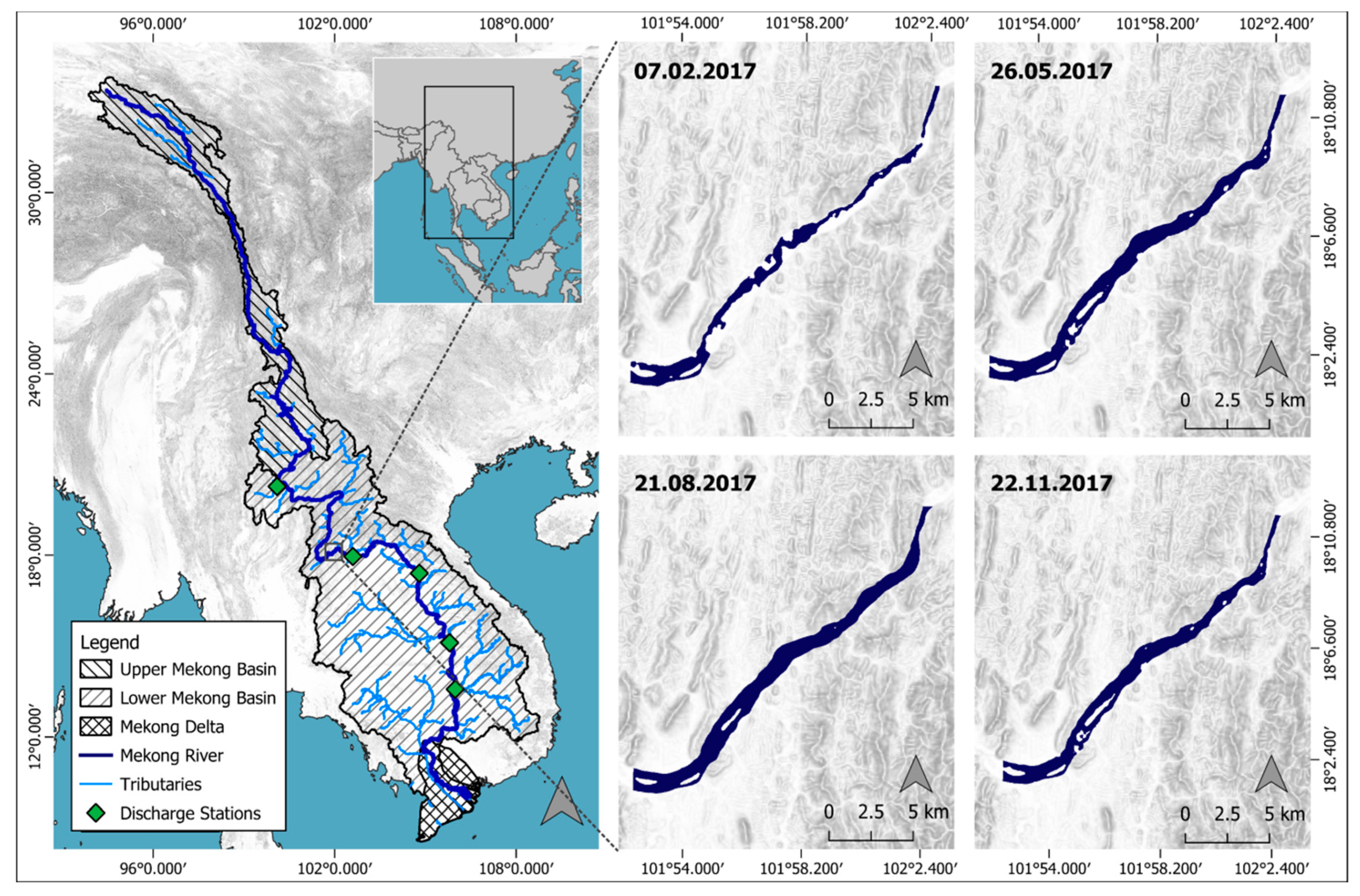
A 28 km long river section located in the Lower Mekong River Basin, 70 km west of Laos’ capital city Vientiane, was selected for estimating the discharge in this study (Figure 1). This area was chosen because the river shows a great variety in width within this section throughout the year and because it is in closer proximity to a discharge station compared to similar sites. During the dry season, the riverbed has a braided character, with a perennial main channel and several intermittent side channels, partly cut off by islands and vegetation as observed using optical satellite images. During the wet season, the riverbed is completely inundated. Throughout the year, the Mekong River shows a highly dynamic flood pattern at this location with an average width of around 500 m during the dry season and around 700 m during the wet season. In this regard, Sentinel-1 image data with its 10 m pixel spacing is capable of detecting even slight river width changes. The average widths are calculated using RivWidth_v04 software tool from Pavelsky and Smith applied on water masks derived from Sentinel-1 SAR images and the Otsu thresholding method [33,34]. The drainage area of this river location is around 4815 km², the mean annual discharge is around 4500 m³/s, based on the values of the nearest gauging station, and the slope along the river section is ~0.05%. Along the selected river section there are no major in- or outflows, fulfilling the criteria of mass-conservancy required for the applied method. The nearest in situ measuring station we had access to is located about 100 km downstream in Vientiane and is used for validation data.

3. Materials and Methods

3.1. Data

3.1.1. In Situ Gauging Station

In situ data on daily river level and discharge at the measuring station LA 011901 (17°57′26.0′’N, 102°36′4.0′’E) in Vientiane was kindly provided by the Mekong River Commission (MRC) and used for validation purposes. The river level data covers the period from January 1965 to December 2018, the discharge data the period from January 1913 to December 2006 (Figure 2). As the in situ discharge data is not covering the Sentinel-1 time period, it is extended until 2018 by correlating it with the water level data.

3.1.2. The Joint Research Center Global Surface Water Dataset

The Joint Research Center (JRC) Global Surface Water (GSW) dataset provides information on the temporal and spatial extent of open surface water bodies between March 1984 and October 2015 (can be accessed under https://global-surface-water.appspot.com/download). Covering 99.95% of the Earth`s land surface, the JRC GSW dataset consists of 380 classified raster images, which provide monthly data on water coverage of land surface with a spatial resolution of 30 m [35]. For this purpose, each pixel within the time series data of the Landsat archive (Landsat 5, 7, and 8 Level 1T) were classified either as open water, land or non-valid observation, using an expert system classifier. It is based on a procedural sequential decision tree, using both the multispectral and temporal information of the Landsat time series.
In this study, the water seasonality layer of the JRC GSW data set is used, which describes each year’s interannual water coverage and indicates the number of months water was present in each pixel. The year between October 2014 and October 2015 was used as it is given as an example data layer within the JRC GSW dataset, accessible via the GEE. Gaps in the observation period (e.g., due to heavy cloud cover during the wet seasons) are compensated by an estimation of potential permanent surface water. For this purpose, all pixels ever classified as permanent (12 months water coverage) during the entire observation period of 32 years are used and combined with those from the specific year [35].

3.1.3. Sentinel-1 SAR Time Series Data

A total of 318 scenes of Sentinel-1A and Sentinel-1B dual-polarized (VV + VH) data in Interferometric Wide-Swath Mode (IW) and Ground Range Detected High Resolution (GRDH) format [36] for the period from January 2015 to December 2018 were selected (Figure 3). Using Terrain Observation with Progressive Scans SAR (TOPSAR), the standard mode IW captures three sub-swaths, combining it into a 250 km swath with a spatial resolution of 5 m by 20 m. The GRDH products are resampled into a 10 m by 10 m pixel spacing. The earth observation data was retrieved from the GEE web platform [37], which provides already preprocessed Sentinel-1 imagery undertaken by the Sentinel-1 Toolbox SNAP [38]. The processing includes thermal noise removal, radiometric calibration, terrain correction using Shuttle Radar Topography Mission (SRTM) Version 3.0 Global 1 arc second dataset (SRTMGL1), and converting backscatter values to decibels (dB) using log scaling [28].
Following the same orbital plane, the satellite pair of Sentinel-1 A and Sentinel-1 B are mapping the Earth’s surface using a synthetic aperture radar instrument with a frequency of 5.4 GHz (C-band). Launched in April 2014 and April 2016, the Sentinel-1 satellites have a revisit time of 12 days each, combined 6 days, and assure a continuous image recording under all weather and illumination conditions [39,40]. With the upcoming launches of the two additional satellites Sentinel-1 C and Sentinel-1 D, they provide a temporal and spatial high-resolution time series for globally mapping and monitoring rivers. Compared to optical images, the use of SAR images is particularly advantageous here, as they enable cloud and weather-independent Earth observation. Especially in tropical and subtropical areas, this allows the creation of a continuous time series as well, as these regions can be monitored constantly, which is not feasible using optical images as heavy cloud cover during the rainy season causes very large time gaps.

3.2. Methods

3.2.1. Mapping Highly Dynamic River Segments

Highly dynamic river regions, where a change in discharge is strongly related to a change in the river width, needed to be identified along the Mekong River. In this regard, a systematic analysis of the temporal and spatial riverbed inundation dynamics was performed using the seasonality layer of the JRC Global Water data set. The seasonality percentage was computed for given river segments by calculating the ratio between the number of pixels with less than 12 months water coverage and the number of all pixels. River segments with a high percentage are more dynamic with respect to their spatial inundation pattern and their river widths react more sensitively to changes in discharge. These regions, referred to as highly dynamic river regions, have a significant difference between the river width during low flow conditions compared to the river width during peak flow conditions, and are therefore more suitable as study areas than river segments with a low seasonality percentage. The analysis was carried out on multiple scales, calculating the seasonality percentage for river segments with a length of 100 km, 50 km, 25 km, 10 km, and 5 km, respectively.
The analysis contains multiple data processing steps, starting by clipping the JRC GSW seasonality raster to the Mekong River region, using a buffered shapefile of the river courses within the GEE. The raster was vectorized and the river channel polygon was selected by its size, which denotes the largest. Due to the small river size in the upstream regions, parts of the river are not represented continuously in the seasonality raster. Missing river parts were therefore added manually and adjacent tributary rivers, inundation areas and artifacts were filtered out.
To create river segments of equal length, a rough centerline vector is created. Orthogonals are calculated in the respective distance for subdividing the channel polygon by using simple trigonometry, based on the method of Pavelsky and Smith [34].
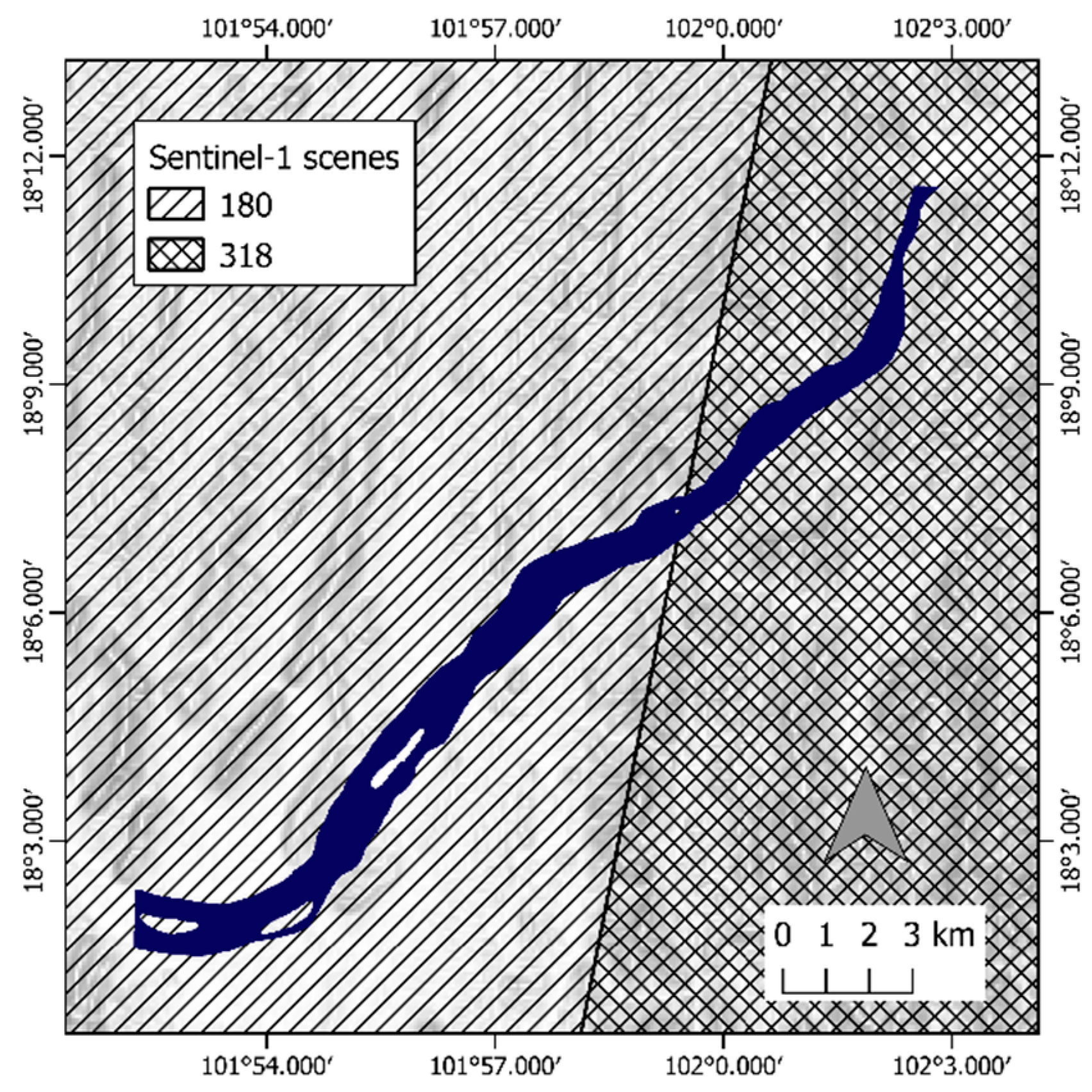
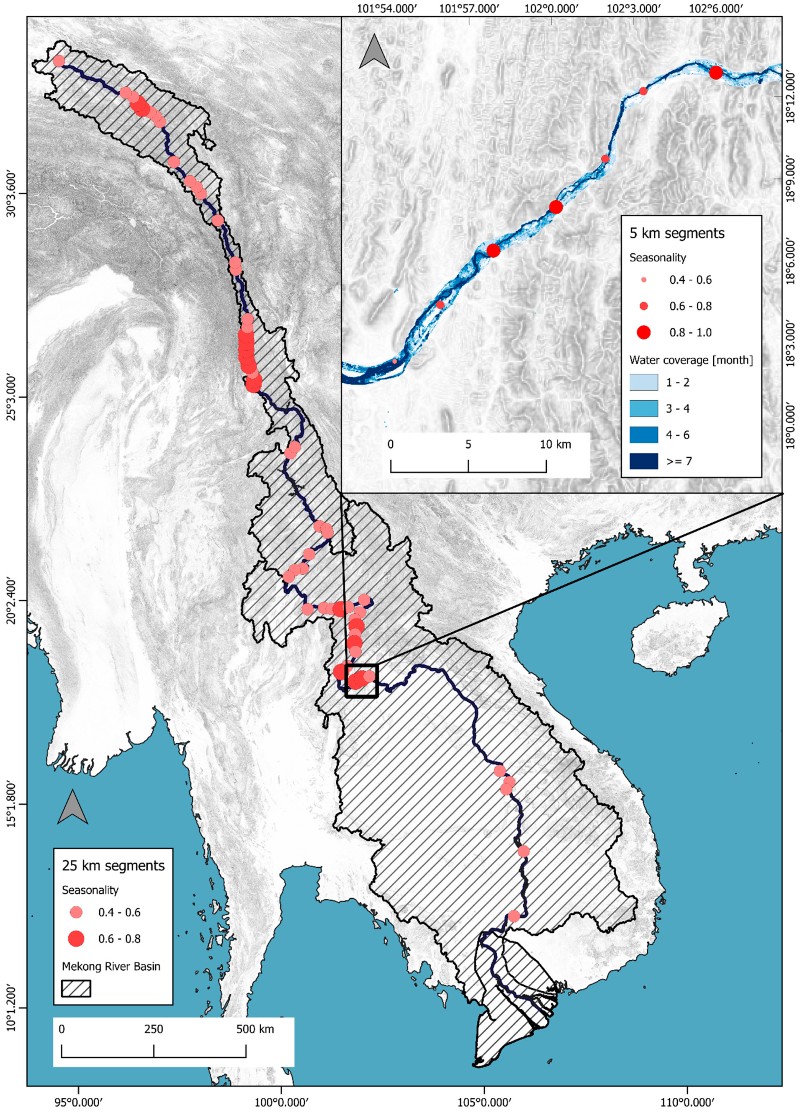
As the width of the river channel polygon is varying along the river course, the length of the transects needs to be variable. Therefore, an algorithm is used, which selects the last intersection of each transect with the river polygon on both sides of the centerline and sets it as the transect’s length. Especially in multichannel river regions, this method is necessary for obtaining a correct segmentation (Figure 4). As shown in Figure 5, most of the highly dynamic river regions are located in the Upper Mekong River Basin as well as the upper part of the Lower Mekong River Basin.

3.2.2. Correlation of Discharge and Water Level Data

The in situ measured discharge data covers a period from January 1913 to December 2006 and therefore does not cover the period of the Sentinel-1 data, which is available since September 2014 (Figure 2). For this reason, the in situ measured data was extended by correlating it with the water level data, which is available until end of 2018 and matches the period of the SAR time series data. The correlation was performed with data from 1965 to 2001 using a third-degree polynomial function with r² = 0.9797.
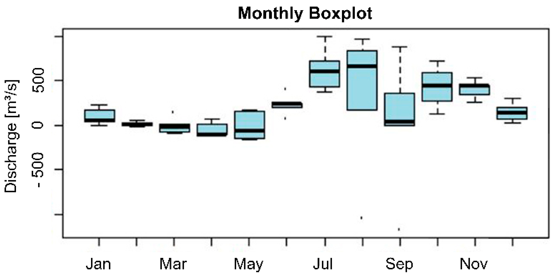
For validation purposes, discharge data is generated from the water level measurements using the fitted third degree polynomial function for the period 2002 to 2006 and compared to the in situ measured discharge values (Figure 6 and Figure 7). A modest overestimation of discharge occurs during the flood season, mostly in the months of July, August, October, and November. With an average overestimation of ~360 m³/s, the deviation is around 4.7% of the mean discharge within these months. The deviation for the dry season months is lower, at around 60 m³/s, or 3.1% of the mean discharge of the months.
Using the fitted third degree polynomial function, referred to as , the discharge for the period from 2015 to 2018 was calculated based on the related water level data. As shown in Figure 8, the river has a distinct flood pulse pattern during the wet season at this location. The maximum flood-peak related discharge is observed in August 2018 with 18,676 m³/s. The minimum low-flow discharge is in February 2016 with 1346 m³/s. The mean discharge is 4558 m³/s.

3.2.3. At-Many-Stations Hydraulic Geometry

The method used in this study to calculate the flow rate from river width measurements is based on the studies of at-many-stations hydraulic geometry (AMHG) of Gleason and Smith [18]. Starting with the studies of hydraulic geometry by Leopold and Maddock [23], river width (w), is related to discharge (Q) by the power-law functions:
w = a Q b
where the parameters a and b are derived empirically through in situ measurements of both river discharge and river width. Using the so-called rating curve method, a power-law function is fitted to the correlated measurement data and the respective coefficients are obtained [41]. This relationship, known as at-a-station hydraulic geometry (AHG), is considered to be site-specific and unstable over time, as it is mainly influenced by geomorphological characteristics of the river bed [42]. By plotting coefficient pairs from various spatially distributed cross sections along a river, Gleason and Smith [18] revealed that the coefficients are not randomly distributed and rather follow a log-linear relationship, the so called at-many-stations hydraulic geometry (AMHG). Although this relationship is a consequence of imposing power law functions for AHG at cross sections, which intersect near the same values of discharge and width, it can be used for estimating discharge through repeated river width measurements within a mass-conserved river reach [24].

3.2.4. Discharge Estimation Workflow

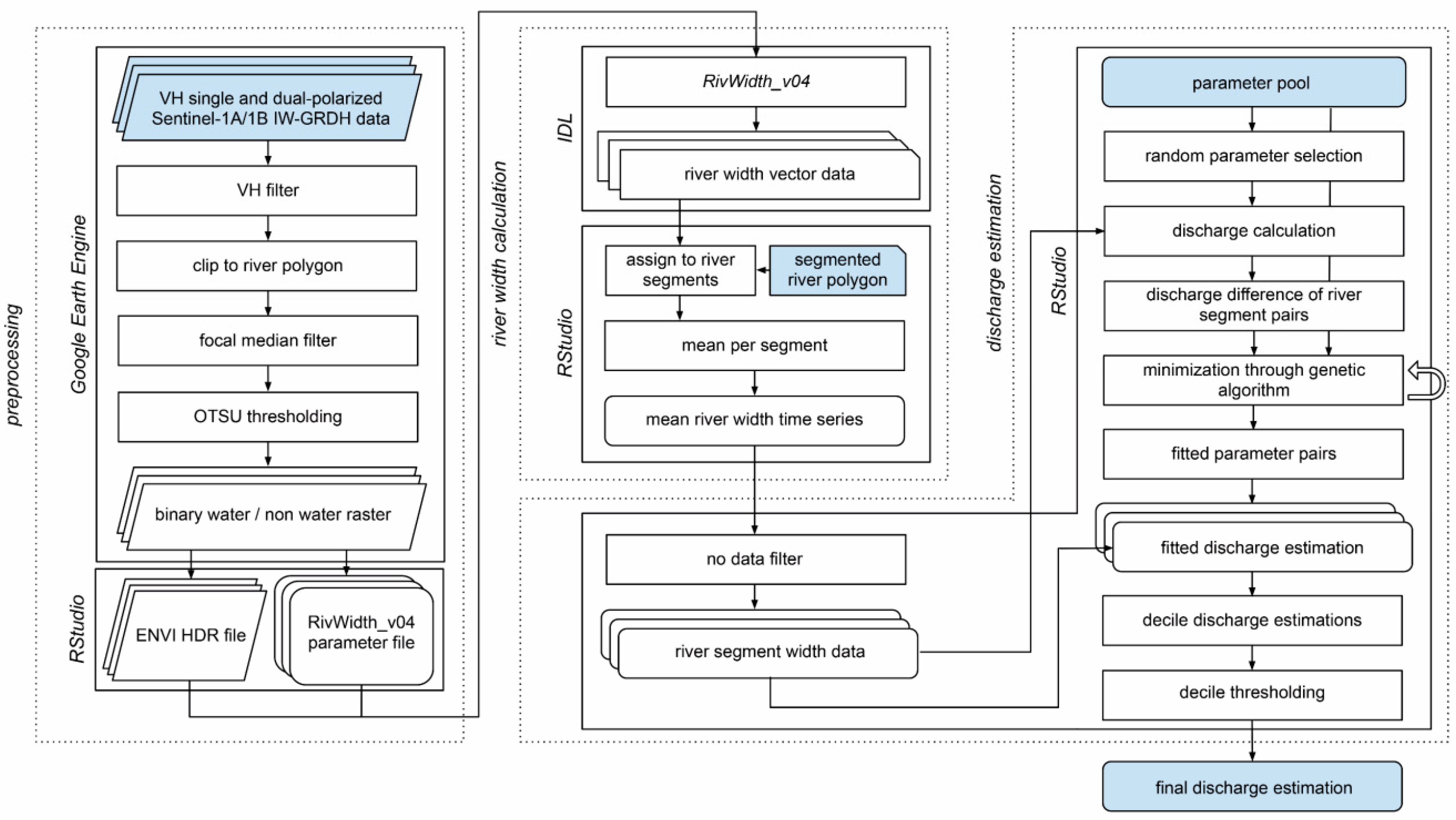
The workflow for estimating discharge from river width measurements for a selected river reach can be divided into three main parts: (1) Preprocessing Sentinel-1 SAR data, (2) river width measurements, and (3) the actual discharge estimation (Figure 9). Most of the preprocessing work is done within the GEE, allowing cloud-based geospatial analysis of satellite data and CPU-intensive operation in a considerably shorter time and downloading only the required output information for further analysis. The consecutive river width measurements are mainly accomplished by using the RivWidth_v04 software tool from Pavelsky and Smith [34] in the programming language IDL. All other processing steps, in particular the discharge estimation, are done in the programming language R using RStudio.
All available VH dual-polarized Sentinel-1A/1B IW-GRDH images acquired in descending mode and covering the study region were selected for further processing. For the period from 1 January 2015 to 31 December 2018, a total amount of 318 images were obtained. In a next step, the images were clipped to the buffered river polygon vector within the boundaries of the study area. It was important that the clipped Sentinel-1 image rasters contain a sufficient proportion of no-water pixels, as it increases the accuracy of the water classification afterwards.

Spatial Filtering

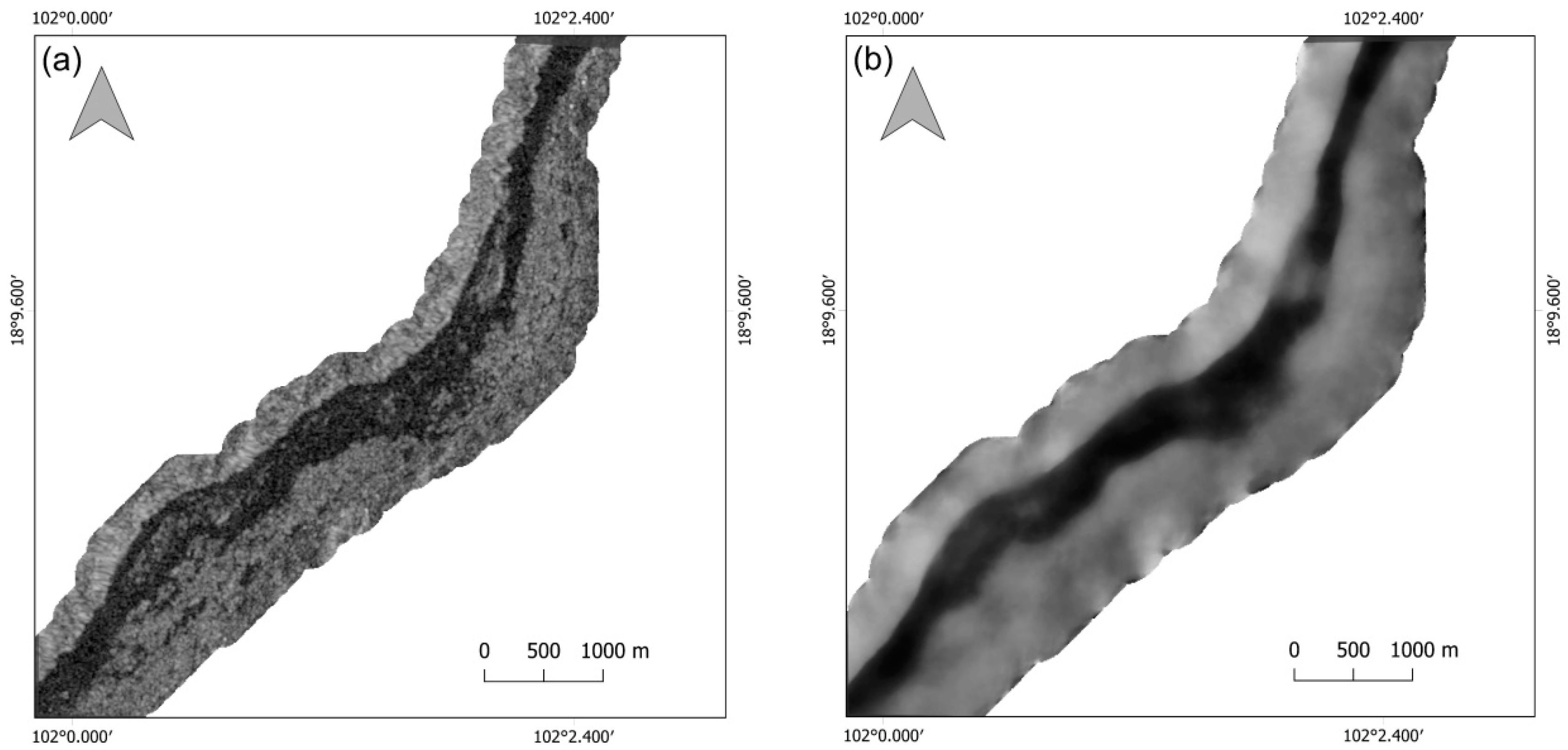
A denoising filter was used to reduce the speckle in the single-date SAR imagery and to improve the image quality (Figure 10). The main objective is to increase the separability between water and non-water pixels. In this study, a focal median filter with a kernel size of 15 x 15 pixels was applied to all Sentinel-1 SAR images, calculating for each pixel the median from all neighboring pixel values and rewriting it into the original pixel. Its rapid performance makes is suitable for cloud-processing large time series data sets as well as it better preserves the edges of objects, compared to the focal mean filter, which is of high interest for measuring river widths [43].

Water Thresholding

After noise reduction, the SAR images were classified into water and non-water classes by applying OTSU’s automatic image thresholding method. The method is considered best for surface water classification, based on the results of Ottinger et al. [44], which tested the thresholding methods (1) Isodata [45], (2) Li [46], (3) Yen [47], (4) Otsu [33], and (5) adaptive thresholding [48] using Sentinel-1 images. The method assumes that pixel values can be divided into two distinct classes by calculating a threshold value from its bimodal histogram that optimally separates both classes [33].

RivWidth_v04 Software Tool

The software tool RivWidth_v04 was created for the continuous river width measurements of a river channel from raster images [34]. It is written in the ITT Visual Information Solution (ITTVIS) IDL programming language (downloaded at http://uncglobalhydrology.org/rivwidth/). The tool requires a binary water mask in ENVI format as an input file, where water pixels are classified with 1 and non-water pixels with 0. From this input file a water channel mask was calculated, differentiating between the river boundary and its surrounding [49]. As the Mekong River is braided within the study region, we set the software’s related parameter to 1.
The operation of the RivWidth software tool can be divided into two parts: (1) Derivation of the river centerline and (2) pixelwise calculation of the river width. For the derivation of the centerline, an algorithm based on the Marr–Hildreth technique [50] is used, calculating the shortest distance for every water pixel to non-water pixels [34]. In a next step, the obtained distance raster is convolved, using a bidirectional Laplacian filter, resulting in the final river centerline. The river width is calculated using orthogonal transects for every pixel with a predefined length. Along these transects, the Euclidean distance is measured between the two intersections of each transect with the first non-water pixel of the channel mask [34], which represent the left and right bank of the river. For braided river sections which contain multiple channels, the v04 version calculates multiple centerlines and river widths [49].

River Segment Assignment and Mean

As the centerline is calculated based on each water channel mask, it differs in length, shape and its start- and endpoint. For a continuous and comparable time series of the river width, the calculated river centerlines were assigned to a river channel polygon, which is divided into segments of 100 m length. For a total number of 280 segments (referring to the 28 km long river study area), the mean value of all centerlines for each segment is calculated. For river sections with more than one river channel, multiple separate centerlines are created. In these cases, the total width of the channel segment is the sum of the mean of both width vectors (Figure 11).

River Segment Filtering

As some Sentinel-1 scenes cover only parts of the study area (see Figure 3), the individual river segments have a different number of width measurements. Furthermore, the start- and endpoints of the centerlines calculated by the RivWidth software are not the same, which also leads to a different number of width measurements. In order to ensure that the different number of measurements does not interfere with the subsequent optimization, only segments which exhibit an equal and comparable number of measurements were utilized for the subsequent analyses. For this reason, 65 segments were selected for the continuing steps, each containing a total of 272 width measurements.

Genetic Algorithm for Optimization

As the discharge within a mass-conserved river section is the same in all river segments, the created river width time series can be used to estimate the respective AHG parameters for each river segment. Using a genetic algorithm (GA), the parameters of each river segment are estimated by minimizing the difference in estimated discharge between all possible river segment pairs, formed by two of each of the 380 river segments [18]. The GA uses the concept of natural selection by optimizing the characteristics of a population based on their fitting to specific boundary conditions for multiple reproduction cycles. In this study, the basic unit of the GA is a gene, which contains a coefficient pair from a river segment (a – b). For a pair of river segments, their individual genes form a chromosome (a1 – b1 | a2 – b2). In an iterative process, only those chromosomes that have a smaller difference in the respective calculated discharge than the rest will be passed to the next generation. By crossing the selected chromosomes, random gene mutations and added fresh genes, the next generation is created and selected regarding their difference in discharge [18] (Figure 12).
As a first step, a gene pool is formed which contains 10,000 coefficient pairs between −2.3 <= log(a) <= 6.9 and 0 <= b <= 1. These limits were chosen, as they line up with the range of a and b parameters calculated for several rivers by Gleason and Wang [24]. In a next step, for each river segment, 10 genes are randomly drawn from the gene pool. Each gene is used to calculate a discharge time series from the associated river segment width time series. Based on the a priori knowledge of the discharge characteristics of the river region, the minimal allowed discharge is set to 500 m³/s and the maximal allowed discharge to 30,000 m³/s. If the discharge boundaries are not known from historic records, the minimum and maximum discharge (Qmin, Qmax) can be calculated by:
Q m i n   =   w m i n   × 0.5   m d e p t h   × 0.1   m s
Q m a x   =   w m a x   × 10   m d e p t h   × 5   m s
with wmin and wmax as minimum and maximum observed river width [18]. If the minimum and/or the maximum discharge of a time series is not within the limits, a new gene is drawn from the gene pool and tested again until all 10 genes pass the filter for each river segment.
In the next step, 10 chromosomes are formed from these genes for every possible river segment pair and the corresponding difference in discharge is calculated. The chromosomes are ranked according to the smallest percentual discharge difference and the best chromosome is directly passed to the next generation. The other nine chromosomes are formed by selecting genes from the chromosomes by a probability based on their ranking. Here, the least fitting chromosome has a probability of 1/55; the best chromosome has a probability of 10/55. Furthermore, with a probability of 1%, a chromosome is randomly selected in every new generation and each gene is mutated by a random factor. This process is repeated for 20 generations and is done 20 times for each river segment pair, resulting in 200 fitted parameter pairs for each river segment. For each segment the mean value of the respectively 200 a and 200 b parameter is calculated, which are then used to calculate the discharge for each river segment from the related river width time series.

Decile Thresholding

As the genetic algorithm returns 272 discharge estimations for each of the 65 river segments, it generates 17,680 individual discharge values in total. To combine these values into a single discharge time series, we developed a novel decile thresholding method, filtering out over- or underestimated discharge values. By this, we extended the previous discharge estimation method proposed by Gleason and Wang [24] to not require a priori knowledge or proxy assumptions.
The decile thresholding method involves grouping the individual discharge values of each day into the respective deciles in a first step. For every decile group, the mean value is calculated, resulting in 10 mean values per day. To give an example, the mean is calculated from the minimum discharge value to the first decile of each day, one from the first to the second decile and so on. In a next step, combining the respective mean values for the whole observation period in each decile group, resulting in 10 new discharge time series. To combine these 10 discharge time series into one final estimation, the discharge time series are stacked on top of each other at certain thresholds. To derive these thresholds, the individual decile values from each decile discharge time series are calculated. In this regard, the value from the first decile serves as a threshold for the corresponding first decile discharge time series, the value from the second decile serves as a threshold for the corresponding second decile discharge time series and so on. To stack the discharge time series, for the first decile discharge time series (1), the first decile is calculated and values, which are exceeding, are replaced by the values of the second decile discharge time series (2), resulting in a combined discharge estimation (1&2). In a next step, the second decile of the second decile discharge time series (2) is calculated and used as a second threshold. Every value of the combined discharge estimation (1&2), which is above, is now replaced by the third decile discharge time series (3), resulting in a new combined discharge simulation (1&2&3). In this manner, all the other decile discharge time series are added to create the final discharge estimation.
The combination of the discharge simulations is based on the assumption, that for some river segments, the correlation of river width and discharge is higher in the low flow regime and for other in the high flow regime. In this regard, some simulations are more representative regarding their low flow discharge estimations or their high flow discharge estimations, respectively. By dividing the simulations into decile intervals, only simulations with a similar correlation in the respective interval are averaged. Combining the respective simulations, discharge values from the best correlation are taken into account, by dismissing discharge values from segments where flow width no longer correlates.

3.2.5. Optimized AMHG Discharge Estimation

For comparison, the discharge was estimated using the optimized AMHG discharge estimation method proposed by Gleason and Wang [24]. Taking the mean value of the 200 a parameters derived from the genetic algorithm for each river segment, the corresponding b parameter is calculated using the proxy AMHG function
b =   0.3 log ( a ) + ( 0.3 w ¯ i )
with w ¯ i being the mean value of all measured river widths. The discharge is calculated for each of the 65 river segments from its corresponding width time series and AHG parameter pair, resulting in 65 individual discharge time series. By taking the daily mean value, the final discharge estimation is created.

4. Results

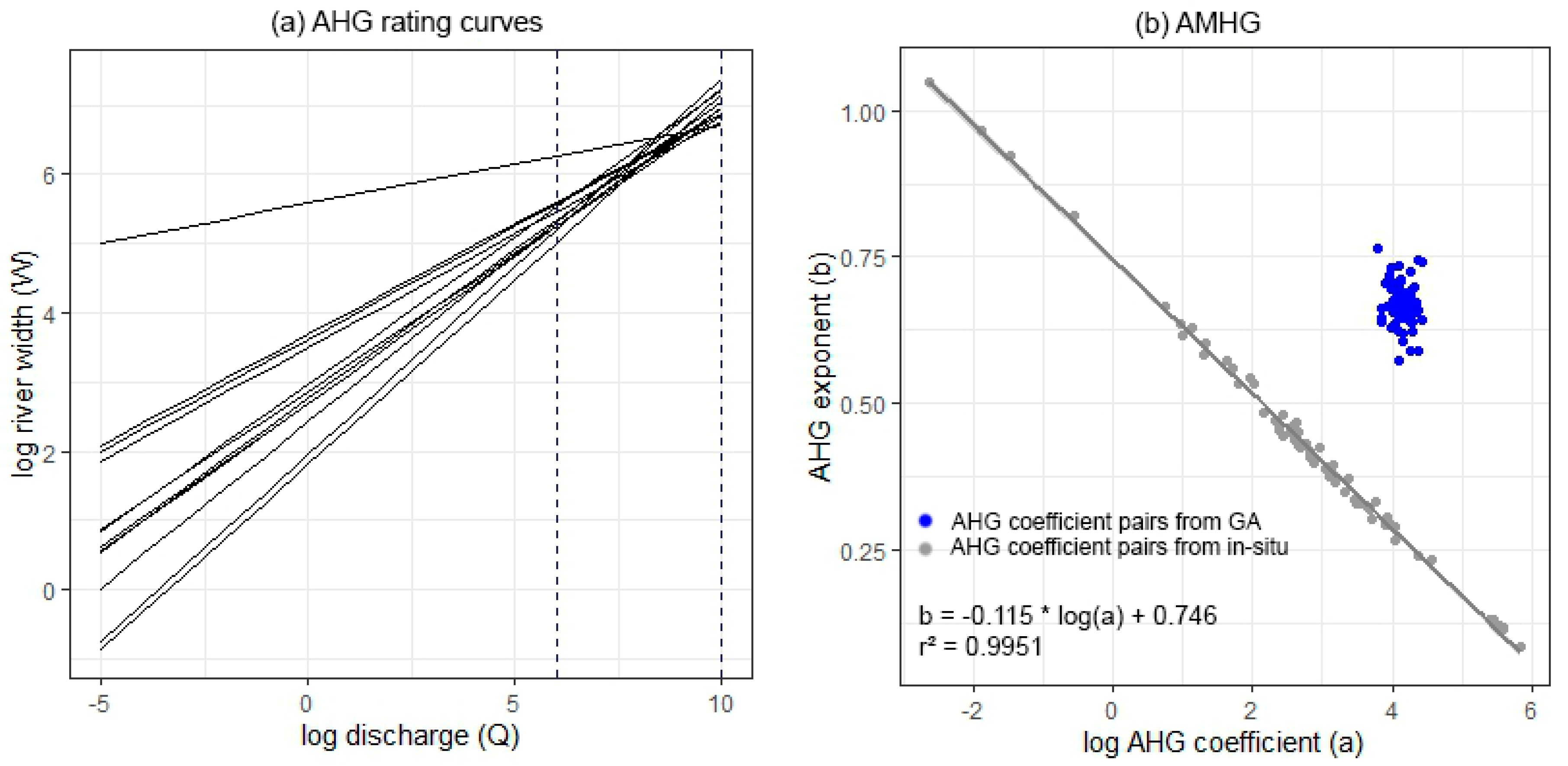
Based on the in situ discharge measurements, the river segments within the observed river reach exhibit distinct AMHG behavior. Correlating the in situ discharge data to the corresponding river width measurements, the AHG rating curves intersect around the same log(Q) – log(W) values (Figure 13a). As shown in Figure 13b, the AHG parameters (gray points) of the investigated river reach can therefore be described by a log-linear AMHG function (gray line) with b = −0.115 *log(a) + 0.746, which has an r² of 0.9951. The parameters log(a) and b are between −2.6 to 5.8 and between 0.08 to 1.05, respectively. In comparison, the AMHG parameters derived from the genetic algorithm (blue points) are between 3.7 to 4.4 for parameter log(a) and 0.57 to 0.76 for parameter b. With a root mean square error (RMSE) of 0.405, the parameter pairs are not in close proximity to the AMHG function. Furthermore, they do not tend to show an AMHG relationship by themselves, as they appear to be quite clustered. In this regard, the genetic algorithm using completely randomly drawn initial parameters from the parameter pool was not able to generate AHG parameters comparable to the ones observed from in situ data.
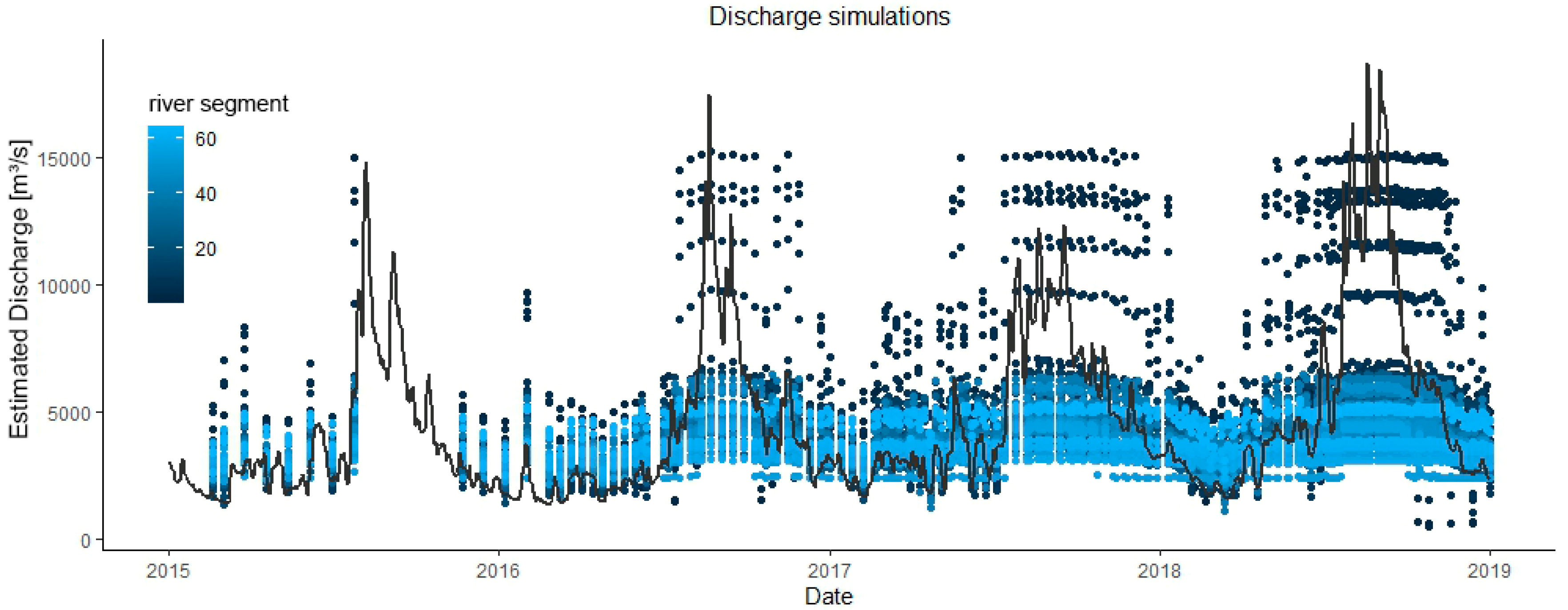
The discharge estimations derived from the AHG optimization show great variability for each day, even though the genetic algorithm decreases the difference in discharge between the river segments (Figure 14). They do not tend to draw a consistent discharge behavior of the river but rather form a daily discharge interval. With an average difference of 5000 m³/s between the highest and lowest simulation value, the simulations are closer together during the dry season than during the rainy season, with a difference of around 10,000 m³/s. The minimal discharge is 473 m³/s, whereas the maximal discharge is 15,237 m³/s; both underestimate the minimum and maximum in situ discharge. Nevertheless, a seasonal pattern can be observed in all simulations, with some simulations having a wider range between minimum and maximum discharge and a larger variance in their discharge values.
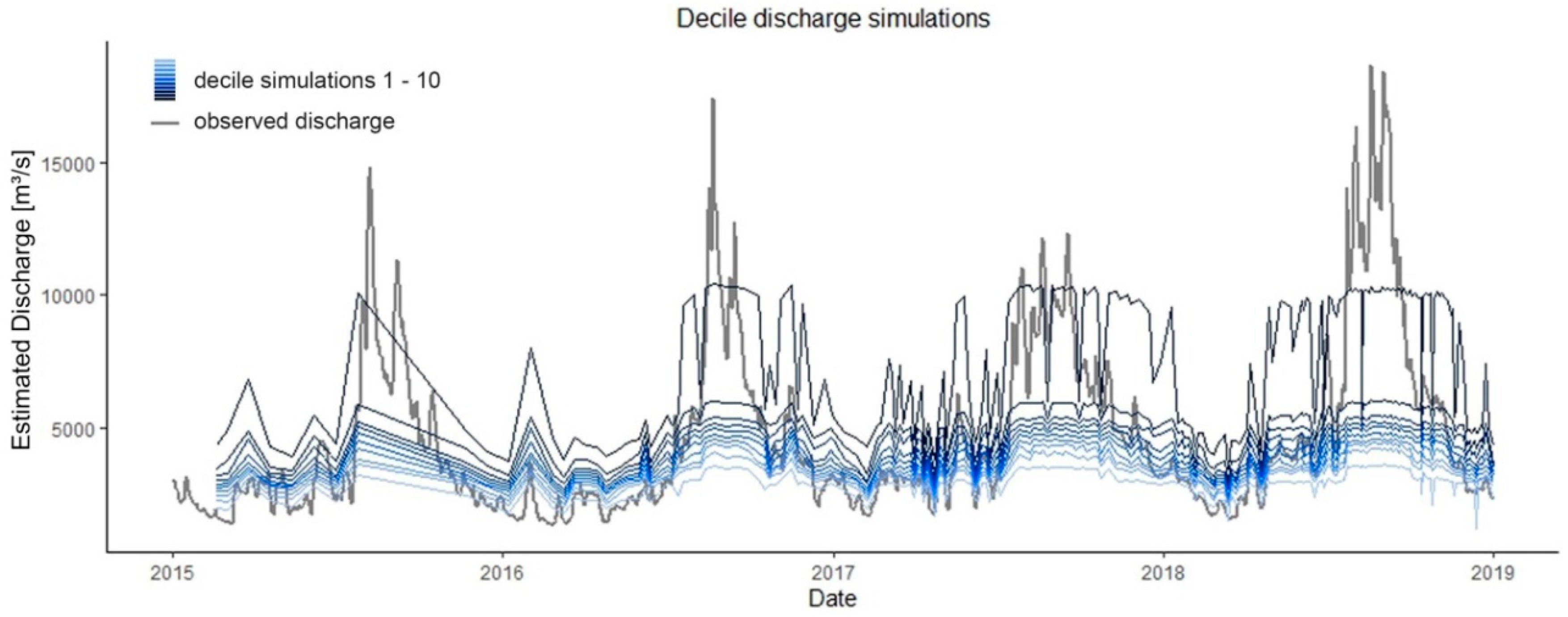
The calculation of the mean decile simulations results in ten simulations which have a certain discharge range, where the difference between estimated and observed discharge is smallest, compared to the other simulations within the same range (Figure 15). The simulations follow a similar pattern and are superimposed, with the lowest decile simulation having the lowest discharge values and the highest decile simulation having the highest values. The difference between the single simulations is not equal but tends to be larger for the lowest and the highest decile simulations, especially during the high discharge periods. The mean difference between the first and second simulation, as well as between the eighth and ninth simulation, is around 400 m³/s, whereas the difference between the second to eight simulation is around 170 m³/s to 300 m³/s. The greatest difference is between the ninth and tenth simulation with around 2200 m³/s and a maximum difference of 4450 m³/s.
By combining the decile discharge simulations into a single final simulation, the estimated discharge largely corresponds to the observed discharge values, significantly improving the estimation of low flow and peak flow compared to the optimized AMHG method (Figure 16). The minimum discharge is 1197 m³/s, the maximum discharge is 10,439 m³/s as well as the overall mean is 4485 m³/s. Comparing the simulation to the observed discharge, it is about 8236 m³/s below the maximum observed discharge value, 147 m³/s below the minimum observed discharge value and just 73 m³/s below the observed mean discharge. Regarding the optimized AMHG discharge estimation derived from the method of Gleason and Wang [24], it shows greater deviations to the validation data, underestimating the high flow discharges as well overestimating the low flow discharges to a far greater extent (Figure 16). Here, the minimum discharge is 2558 m³/s, the maximum discharge is 5488 m³/s and the mean discharge is 4260 m³/s, resulting in a respective deviation of 1213 m³/s, −13,188 m³/s and −298 m³/s to the minimum, maximum and mean of the validation data.
Comparing the discharge values of the simulations with the observed values on the respective day of recording, the decile thresholding method shows a root mean square error (RMSE) and relative root mean square error (RRMSE) almost half as large as the optimized AMHG method, with 1706 m³/s versus 3074 m³/s and 19.5 % versus 38.5%. The median error of the decile thresholding method is 152 m³/s, which is more than three times smaller than the median error of the optimized AMHG method with 538 m³/s. Looking more closely at the performance of the simulation grouped by months, for the dry season months, both simulations have much lower errors than during the wet season (Figure 17). For the months November to June, both methods show here in general smaller interquartile ranges, less extreme outliers, and smaller median errors, while the discharge is always overestimated. The best results from the decile thresholding method are obtained for the months of May and June with RRMSE of 10.9% and 10.8%. The optimized AMHG method achieves its best results in the months of June and November with a RRMSE of 21.9% and 17.0%.
Looking at the months of July to October, which are characterized by the occurrence of monsoon-related flood peaks, the differences between estimated and observed discharge are greatest in both discharge estimations. In these months, both methods have far greater interquartile ranges and more extreme outliers, while always underestimating the observed discharge. For August and September, the months with the greatest discrepancy between simulation and observed discharge values, the decile thresholding method has a RRMSE of 28.8% and 26.5%. The optimized AMHG method has a RRMSE of 53.7% and 50.0% in the same months, which is almost twice as high. A complete overview about the performance of both methods is displayed in Table 1.

5. Discussion

With an overall RRMSE of 19.5%, the decile thresholding method achieves a level of performance almost a twice as good at the study region as the optimized AMHG method, with an RRMSE of 38.5%. As both methods have comparable mean discharge values of 4485 m³/s and 4260 m³/s, and are therefore close to the observed mean of 4558 m³/s, their main difference can be found in the estimation in low and high discharge ranges. With minimum discharge of 2558 m³/s and a maximum discharge of 5488 m³/s, the optimized AMHG method is not able to represent the full range of observed discharge values, ranging between 1345 m³/s and 18,676 m³/s. In this way, it systematically overestimates both the low flow discharges and underestimates the flood discharges, which is clearly visible in Figure 16 and Figure 17. In comparison, the decile thresholding method is able to improve the estimation of both the low flow discharge as well as the peak discharge. With a minimum estimated discharge of 1197 m³/s and a maximum estimated discharge of 10,439 m³/s, it can cover the observed discharge range comparably better. For the distribution of discharge deviations, a decrease of around 70% can be seen regarding the mean error (152 m³/s to 538 m³/s) as well as the interquartile range is decreasing around 53% (−663 m³/s to 387 m³/s and −1354 m³/s to 891 m³/s).
Even though the methods are site specific, the results of the decile thresholding, using 272 observations, are comparable to the optimized AMHG discharge estimations in Gleason and Smith, with RRMSE of 20%, 23%, and 30% for respective river sites at Athabasca River, Mississippi River, and Yangtze River using up to 20 observations [18]. Using our novel proposed method, high numbers of observations do not lead to relatively inferior performances as described in Durand et al. [19], which tested the optimized AMHG method with up to 365 observations for 16 different river sites, achieving RRMSE ranging between 11% to 176.6% with a mean RRMSE of 80.9%. The weaker performance of the optimized AMHG method is caused by the increasing number of observations, which leads to several issues with the AMHG. On the one hand, the proposed AMHG proxy by Gleason and Wang [24] leads to an ineffective AHG optimization. On the other hand, as an increasing number of observations cover a yearly or greater period, the different AHG behavior of wet and dry season becomes a problem within the optimization process [19]. Both problems can be observed as well on the discharge estimation derived from optimized AMHG method in our study region. Using the AMHG proxy function with a slope of −0.3 and 1.91 as intercept, it significantly differs from the AMHG function with a slope of −0.115 and intercept of 0.746 derived from the in situ measurements. In this regard, the proxy AMHG function is not representative for the study site and therefore gives misleading discharge estimates. Furthermore, by taking the mean of all discharge estimations derived from each river segment, the different AHG behavior of wet and dry seasons cannot be coped, resulting in both an overestimation of the low flow discharge as well as an underestimation of peak flow discharge. Even though the later problem also applies to the decile thresholding method, as both use the same initial AHG parameters derived by the genetic algorithm optimization, the decile thresholding method can mitigate this problem. By grouping the discharge estimations into discharge ranges, dry and wet season discharge is represented by different river segments. The calculation of the decile simulations and their combination into a final discharge estimation uses therefore discharge estimations from river segments whose AHG parameters are more fitting for the related discharge range. By this, a decrease of 60% of RRMSE for the dry season months and 39% of RRMSE for the wet season months can be achieved using the decile thresholding method compared to the optimized AMHG method. In this regard, the method can further be incorporated into the upcoming SWOT satellite mission. As river width, stage, and slope measurements will be available, Hagemann et al. [51] proposed novel approach estimating river discharge by using both Manning equation and adding the AMHG method, if the river reach has a high percentage of intersecting AHG curves. Following the same idea, the decile thresholding method can be incorporated into a SWOT adapted method based on Manning equation, if the AMHG behavior is strong in a river reach.
Looking at the dry and wet seasons, there is a clear difference in performance of the discharge estimates, especially regarding the flood peaks. Considering only the months where no flood peak discharge is occurring (Oct–Jun), the accuracy of the decile threshold discharge estimation increases to a RRMSE of 16.0%, while the optimized AMHG method follows the same trend, with an increased accuracy with a RRMSE of 34.5%. This is in line with the trend observed in Gleason and Hamdan [26], reducing the RRMSE from 56% to 28% for an AMHG discharge estimate of the Ganges River considering only the dry season months.
While the decile thresholding method achieves good results in the low-flow range, the peak flows are almost always underestimated with both methods. Looking at the flood peak maxima, the estimated discharge values of the decile thresholding method do not exceed a certain level at around 10,000 m³/s. This is particularly evident in 2018, when the observed discharge exceeded this level in the months of July, August and September. While the observed values vary, the estimated values remain mostly constant around 10,000 m³/s. This characteristic also occurs in the optimized AMHG method, where it reaches its limit at ~5500 m³/s. Due to a lack of correlation between discharge and river width at this discharge level within the corresponding river segments, the estimated discharge is not increasing. The reason for this is found in the underlying shape of the riverbed. If there is no river width change, the method for estimating the river discharge reaches its physical limits. Another related issue is that AHG only describes inbank flow conditions, as overbank flow is driven by other physical parameters [27]. Therefore, the estimation of peak flood discharges causing overbank flow must be managed with other methods. Using floodplain hydraulic geometry, the extent of floodplains along a river course for specific peak discharges can be modeled based on a digital elevation model (DEM) and historic discharge records [27,52]. Reversing this method, measuring the width of floodplain segments can be used to estimate the related peak discharge. Here, future research combining both methods for estimating discharge could be a promising way coping with the underestimation of flood peak discharge.
While the overall accuracy can be increased due to the calculation and combination of decile simulations, in some cases this method does not give the best result possible. This limitation is evident in particular in July 2015, where the final discharge estimation shows a low value derived from the ninth decile simulation, although the discharge estimation from the tenth decile simulation is more consistent to the observed discharge (Figure 16). To avoid these errors, the thresholding should be more closely adapted to the individual hydrological pattern, e.g., for each hydrological year and not just based on data from the total discharge.
The AHG parameters derived from the genetic algorithm do not match the AHG parameters derived from in situ discharge observations. The estimates from the genetic algorithm are all in the range from 3.7 < log(a) < 4.4 and 0.57 < b < 0.76 while the range of the AHG parameters from the in situ measurements range from −2.6 < log(a) < 5.8 and 0.08 < b < 1.05 (Figure 13). In addition, the a and b parameter pairs do not show the linear correlation of the AMHG function. Thus, the genetic algorithm is not able to correctly calculate the respective AHG parameters of the segments, but rather provides adjusted, very similar parameters. As the genetic algorithm only reduces the difference in discharge between the river segments, the optimum does not necessarily result in AHG parameters comparable to the in situ measured ones. Furthermore, the genetic algorithm could have also fallen into a local optimum, even though this issue was addressed using the random mutation of AHG pairs. Using the bayesian inference method for AMHG-based discharge estimation as proposed in Hagemann et al. could improve the calculation of AHG parameters, as it tends to show lower maximum RRMSE values as well as fewer outliers [51]. Nevertheless, as this method also tends to have higher minimum RRMSE values, further research on both optimization methods should be performed, as it could improve the related discharge estimation. Nevertheless, the estimated AHG parameters for each river segment generally provide suitable results for a specific discharge range. As the AHG parameters differ for the wet and dry season, the approach of considering individual river segment simulations for different discharge ranges gives better results than using all river segment simulations for the entire range of discharge.

Strength and Limitations

This paper mainly deals with the evaluation of river discharge estimations from river width time series. Nevertheless, the measurement of the river width using remote sensing methods on Sentinel-1 SAR data has a significant influence on the results of the discharge estimation. Starting with the mapping of highly dynamic river regions, the segment length for calculating the seasonality percentage is highly affecting the identification of these regions. In this study, the river region was selected due to its high seasonality percentage for both 25 km and 5 km segments and its proximity to an in situ discharge station. Developing a systematic approach for identifying suitable river regions with an adaptive segment length for calculating the seasonality percentage would be necessary for applying the method on a global scale. In this regard, also the minimum seasonality percentage for which the discharge estimation method yields good results should be defined. The same is true for the length of the investigated river reach and the number of individual river segments used in the genetic algorithm. As shown in this paper, the use of 65 river segments, with a width of 100 m and within a 28 km long river reach is able to give reasonable results for the discharge estimation. As this number is based on the limitations of Sentinel-1 images and the output of the RivWidth_v04 software, it does not necessarily give optimal results. More detailed studies, on how the number of river segments and the chosen river reach affects discharge estimation could therefore further improve the discharge estimation. Regarding the remote sensing of river width using Sentinel-1 images, speckle has a major impact on the water classification. Especially if the boundary between water and river bank is not clear but is ambiguous due to bank vegetation, partial flooding or abandoned river channels, the speckle can lead to major misinterpretations of the actual river width. Using the focal median filter, the speckle could be efficiently reduced, still losing information by blurring the river boundaries (Figure 10). As different methods for speckle filtering are developed and applied in remote sensing, a detailed consideration of the most suitable filtering method for the purpose of river width measurements should be made. Furthermore, as our method is applied on a single river reach, further research is needed to apply the decile thresholding method on various river reaches worldwide and comparing it to existing spaceborne discharge estimation methods to verify our results.

6. Conclusions and Outlook

We present a novel framework for estimating river discharge using river width measurements, Sentinel-1 SAR time series data and a priori knowledge on minimum and maximum discharge. By using exclusively remotely sensed information about the river width, the discharge estimation method shown in this study requires the least amount of input data, compared to other methods which apply spaceborne earth observation data [38]. Using weather-independent Copernicus Sentinel-1 data with a revisit time of 6 days, which enables observations also during the highly-clouded rainy season, a continuous river width and discharge time series could be created over the whole observation period from 2015 to 2018.
With an RRMSE of 19.5% for the entire investigated period and a RRMSE of 16% for just the dry-season months, the decile thresholding discharge estimation performed well compared to the optimized AMHG method proposed by Gleason and Wang [24], with RRMSE of 38.5% and 34.5% respectively. As shown, our novel decile thresholding method can reduce the error both in the low flow as well as peak flow discharge range, resulting in a decrease of 60% in RRMSE for the dry season and a decrease of 39% in RRMSE for the wet season. Compared to global runoff products with a mean RRMSE of 40%, the decile thresholding method can lead to a significant improvement in discharge estimation, whereas the optimized AMHG method just gives a marginal improvement [38]. An increased error between observed and estimated discharge caused by a high number of observations, as described in Durand et al. [19], could be partly addressed using the decile thresholding method, whereas it can be observed in the optimized AMHG method. To validate our results, the decile thresholding method should be applied on a global scale at various river reaches and compared to existing methods in further research.
As our proposed method depends on a strong correlation between river width and river discharge, which becomes weaker at higher discharge and overbank flow rates [19], the capacity for improving on the discharge is rather limited with our method. Incorporating other remote sensed data (e.g., river level), can be therefore a promising way to extend the approach for flood peak discharge conditions. Here, also the incorporation of floodplain hydraulic geometry methods for estimating peak discharge from floodplain width measurements should be researched in more detail to overcome this issue.
To further improve the result of the presented method and its applicability on a global scale, a closer look on the individual processing steps should be taken. Developing a methodological approach for selecting appropriate, highly dynamic river regions as well as investigating the necessary amount of river segments for discharge estimation would help to further automate the method and apply it to other river systems. Requiring just river width measurements, the method can be easily applied to other spaceborne data, besides Copernicus Sentinel-1 SAR. By combining multiple spaceborne data sources, optical as well as radar, an almost daily observation interval can be achieved. Furthermore, with the upcoming earth observation satellites with increased spatial resolution, the method can be also applied on smaller rivers as well as it will further improve the detectable correlation between river width and river discharge.
As presented, the described framework has great potential for an automated estimation of discharge on an almost daily basis for river systems worldwide. Especially for large, ungauged basins in remote areas, this method can help provide valuable information for both scientific as well as operational use. Using only a short, highly dynamic river reach to estimate the discharge and runoff from the upstream catchment, this method could be applied on multiple locations along the river. By this, not only the total runoff can be estimated but also the runoff between two highly dynamic locations.
Author Contributions

Conceptualization, D.M., M.O, P.L., and L.R.; methodology, D.M. and M.O.; validation, D.M.; writing—original draft preparation, D.M.; writing—review and editing, D.M., M.O., P.L., and L.R.; visualization, D.M.; supervision, M.O. All authors have read and agreed to the published version of the manuscript.

Funding

This research was conducted as a master thesis at the German Remote Sensing Data Center (DFD) of the German Aerospace Center (DLR). It was carried out within the framework of the project CATCH-MEKONG (FKZ 02WM1338A) funded by the Federal Ministry of Education and Research (BMBF).

Acknowledgments

Special thanks go to European Copernicus Satellite Program for providing free access to Sentinel-1 SAR data; the JRC for the Global Surface Water dataset; the Mekong River Commission for providing in situ gauging station data. Furthermore, we would like to thank Google Earth Engine platform for generating and providing the satellite time series. Finally we would like to thank T. M. Pavelsky for distributing RivWidth software and G. Donchyts for the thresholding script available in GEE.

Conflicts of Interest

The authors declare no conflict of interest.

References

  1. Kummu, M.; de Moel, H.; Ward, P.J.; Varis, O. How close do we live to water? A global analysis of population distance to freshwater bodies. PLoS ONE 2011, 6, e20578. [Google Scholar] [CrossRef] [PubMed]
  2. Cosgrove, W.J.; Loucks, D.P. Water management: Current and future challenges and research directions. Water Resour. Res. 2015, 51, 4823–4839. [Google Scholar] [CrossRef] [Green Version]
  3. Peppard, C.Z. Troubling waters: The Jordan River between religious imagination and environmental degradation. J. Environ. Stud. Sci. 2013, 3, 109–119. [Google Scholar] [CrossRef]
  4. Uereyen, S.; Kuenzer, C. A Review of Earth Observation-Based Analyses for Major River Basins. Remote Sens. 2019, 11, 2951. [Google Scholar] [CrossRef] [Green Version]
  5. Razavi, T.; Coulibaly, P. Streamflow Prediction in Ungauged Basins: Review of Regionalization Methods. J. Hydrol. Eng. 2013, 18, 958–975. [Google Scholar] [CrossRef]
  6. Fekete, B.; Vörösmarty, C. The current status of global river discharge monitoring and potential new technologies complementing traditional discharge measurements. Proc. PUB Kick-off Meet. 2002, 309, 20–22. [Google Scholar]
  7. Arnell, N.W.; Gosling, S.N. The impacts of climate change on river flow regimes at the global scale. J. Hydrol. 2013, 486, 351–364. [Google Scholar] [CrossRef]
  8. Tauro, F.; Selker, J.; van de Giesen, N.; Abrate, T.; Uijlenhoet, R.; Porfiri, M.; Manfreda, S.; Caylor, K.; Moramarco, T.; Benveniste, J.; et al. Measurements and Observations in the XXI century (MOXXI): Innovation and multi-disciplinarity to sense the hydrological cycle. Hydrol. Sci. J. 2018, 63, 169–196. [Google Scholar] [CrossRef] [Green Version]
  9. Stisen, S.; Jensen, K.H.; Sandholt, I.; Grimes, D.I.F. A remote sensing driven distributed hydrological model of the Senegal River basin. J. Hydrol. 2008, 354, 131–148. [Google Scholar] [CrossRef]
  10. Laiolo, P.; Gabellani, S.; Campo, L.; Silvestro, F.; Delogu, F.; Rudari, R.; Pulvirenti, L.; Boni, G.; Fascetti, F.; Pierdicca, N.; et al. Impact of different satellite soil moisture products on the predictions of a continuous distributed hydrological model. Int. J. Appl. Earth Obs. Geoinf. 2016, 48, 131–145. [Google Scholar] [CrossRef]
  11. Hartanto, I.M.; van der Kwast, J.; Alexandridis, T.K.; Almeida, W.; Song, Y.; van Andel, S.J.; Solomatine, D.P. Data assimilation of satellite-based actual evapotranspiration in a distributed hydrological model of a controlled water system. Int. J. Appl. Earth Obs. Geoinf. 2017, 57, 123–135. [Google Scholar] [CrossRef]
  12. Chen, X.; Long, D.; Hong, Y.; Zeng, C.; Yan, D. Improved modeling of snow and glacier melting by a progressive two-stage calibration strategy with GRACE and multisource data: How snow and glacier meltwater contributes to the runoff of the Upper Brahmaputra River basin? Water Resour. Res. 2017, 53, 2431–2466. [Google Scholar] [CrossRef]
  13. Li, Y.; Grimaldi, S.; Pauwels, V.R.N.; Walker, J.P. Hydrologic model calibration using remotely sensed soil moisture and discharge measurements: The impact on predictions at gauged and ungauged locations. J. Hydrol. 2018, 557, 897–909. [Google Scholar] [CrossRef]
  14. Bjerklie, D.M.; Lawrence Dingman, S.; Vorosmarty, C.J.; Bolster, C.H.; Congalton, R.G. Evaluating the potential for measuring river discharge from space. J. Hydrol. 2003, 278, 17–38. [Google Scholar] [CrossRef]
  15. Bjerklie, D.M.; Dingman, S.L.; Bolster, C.H. Comparison of constitutive flow resistance equations based on the Manning and Chezy equations applied to natural rivers. Water Resour. Res. 2005, 41, 17. [Google Scholar] [CrossRef] [Green Version]
  16. Birkinshaw, S.J.; O’Donnell, G.M.; Moore, P.; Kilsby, C.G.; Fowler, H.J.; Berry, P.A.M. Using satellite altimetry data to augment flow estimation techniques on the Mekong River. Hydrol. Process. 2010, 24, 3811–3825. [Google Scholar] [CrossRef]
  17. Michailovsky, C.I.; McEnnis, S.; Berry, P.A.M.; Smith, R.; Bauer-Gottwein, P. River monitoring from satellite radar altimetry in the Zambezi River basin. Hydrol. Earth Syst. Sci. 2012, 16, 2181–2192. [Google Scholar] [CrossRef] [Green Version]
  18. Gleason, C.J.; Smith, L.C. Toward global mapping of river discharge using satellite images and at-many-stations hydraulic geometry. Proc. Natl. Acad. Sci. USA 2014, 111, 4788–4791. [Google Scholar] [CrossRef] [Green Version]
  19. Durand, M.; Gleason, C.J.; Garambois, P.A.; Bjerklie, D.; Smith, L.C.; Roux, H.; Rodriguez, E.; Bates, P.D.; Pavelsky, T.M.; Monnier, J.; et al. An intercomparison of remote sensing river discharge estimation algorithms from measurements of river height, width, and slope. Water Resour. Res. 2016, 52, 4527–4549. [Google Scholar] [CrossRef] [Green Version]
  20. Feng, D.; Gleason, C.J.; Yang, X.; Pavelsky, T.M. Comparing Discharge Estimates Made via the BAM Algorithm in High-Order Arctic Rivers Derived Solely from Optical CubeSat, Landsat, and Sentinel-2 Data. Water Resour. Res. 2019, 55, 7753–7771. [Google Scholar] [CrossRef]
  21. Kouraev, A.V.; Zakharova, E.A.; Samain, O.; Mognard, N.M.; Cazenave, A. Ob’ river discharge from TOPEX/Poseidon satellite altimetry (1992–2002). Remote Sensing of Environment. 2004, 93, 238–245. [Google Scholar] [CrossRef] [Green Version]
  22. Birkinshaw, S.J.; Moore, P.; Kilsby, C.G.; O’Donnell, G.M.; Hardy, A.J.; Berry, P.A.M. Daily discharge estimation at ungauged river sites using remote sensing. Hydrol. Process. 2014, 28, 1043–1054. [Google Scholar] [CrossRef]
  23. Leopold, L.B.; Maddock, T., Jr. The Hydraulic Geometry of Stream Channels and Some Physiographic Implications; Professional Paper No. 252; U.S. Government Printing Office: Washington, DC, USA, 1953. Available online: http://pubs.er.usgs.gov/publication/pp252 (accessed on 20 June 2019).
  24. Gleason, C.J.; Wang, J. Theoretical basis for at-many-stations hydraulic geometry. Geophys. Res. Lett. 2015, 42, 7107–7114. [Google Scholar] [CrossRef] [Green Version]
  25. Biancamaria, S.; Lettenmaier, D.P.; Pavelsky, T.M. The SWOT Mission and Its Capabilities for Land Hydrology. Surv. Geophys. 2016, 37, 307–337. [Google Scholar] [CrossRef] [Green Version]
  26. Gleason, C.J.; Hamdan, A.N. Crossing the (watershed) divide: Satellite data and the changing politics of international river basins. Geogr. J. 2015, 183, 2–15. [Google Scholar] [CrossRef]
  27. Dodov, B.; Foufoula-Georgiou, E. Fluvial processes and streamflow variability: Interplay in the scale-frequency continuum and implications for scaling. Water Resour. Res. 2005, 41, 311. [Google Scholar] [CrossRef] [Green Version]
  28. Google. Sentinel-1 Algorithms. Available online: https://developers.google.com/earth-engine/sentinel1 (accessed on 18 November 2019).
  29. Adamson, P.T.; Rutherfurd, I.D.; Peel, M.C.; Conlan, I.A. The Hydrology of the Mekong River. In The Mekong; Elsevier: Amsterdam, The Netherlands, 2009; pp. 53–76. ISBN 9780123740267. [Google Scholar]
  30. Hoang, L.P.; Lauri, H.; Kummu, M.; Koponen, J.; van Vliet, M.T.H.; Supit, I.; Leemans, R.; Kabat, P.; Ludwig, F. Mekong River flow and hydrological extremes under climate change. Hydrol. Earth Syst. Sci. 2016, 20, 3027–3041. [Google Scholar] [CrossRef] [Green Version]
  31. Lauri, H.; de Moel, H.; Ward, P.J.; Räsänen, T.A.; Keskinen, M.; Kummu, M. Future changes in Mekong River hydrology: Impact of climate change and reservoir operation on discharge. Hydrol. Earth Syst. Sci. 2012, 16, 4603–4619. [Google Scholar] [CrossRef]
  32. Hung, N.N.; Delgado, J.M.; Tri, V.K.; Le Hung, M.; Merz, B.; Bárdossy, A.; Apel, H. Floodplain hydrology of the Mekong Delta, Vietnam. Hydrol. Process. 2012, 26, 674–686. [Google Scholar] [CrossRef] [Green Version]
  33. Otsu, N. A Threshold Selection Method from Gray-Level Histograms. IEEE Trans. Syst. Man Cybern. 1979, 9, 62–66. [Google Scholar] [CrossRef] [Green Version]
  34. Pavelsky, T.M.; Smith, L.C. RivWidth: A Software Tool for the Calculation of River Widths from Remotely Sensed Imagery. IEEE Geosci. Remote Sens. Lett. 2008, 5, 70–73. [Google Scholar] [CrossRef]
  35. Pekel, J.-F.; Cottam, A.; Gorelick, N.; Belward, A.S. High-resolution mapping of global surface water and its long-term changes. Nature 2016, 540, 418–422. [Google Scholar] [CrossRef]
  36. Fletcher, K. ESA’s Radar Observatory Mission for GMES Operational Services; European Space Agency: Noordwijk, The Netherlands, 2012. [Google Scholar]
  37. Gorelick, N.; Hancher, M.; Dixon, M.; Ilyushchenko, S.; Thau, D.; Moore, R. Google Earth Engine: Planetary-scale geospatial analysis for everyone. Remote Sens. Environ. 2017, 202, 18–27. [Google Scholar] [CrossRef]
  38. ESA. The Sentinel Application Platform (SNAP), a Common Architecture for all Sentinel Toolboxes Being Jointly Developed by Brockmann Consult, Array Systems Computing and C-S. 2017. Available online: http://step.esa.int/main/download/ (accessed on 12 May 2019).
  39. Torres, R.; Snoeij, P.; Geudtner, D.; Bibby, D.; Davidson, M.; Attema, E.; Potin, P.; Rommen, B.; Floury, N.; Brown, M.; et al. GMES Sentinel-1 mission. Remote Sens. Environ. 2012, 120, 9–24. [Google Scholar] [CrossRef]
  40. Schubert, A.; Small, D.; Miranda, N.; Geudtner, D.; Meier, E. Sentinel-1A Product Geolocation Accuracy: Commissioning Phase Results. Remote Sens. 2015, 7, 9431–9449. [Google Scholar] [CrossRef] [Green Version]
  41. Sivapragasam, C.; Muttil, N. Discharge Rating Curve Extension–A New Approach. Water Resour. Manag. 2005, 19, 505–520. [Google Scholar] [CrossRef]
  42. Phillips, J.D. The instability of hydraulic geometry. Water Resour. Res. 1990, 26, 739–744. [Google Scholar] [CrossRef]
  43. Rees, W.G.; Satchell, M.J.F. The effect of median filtering on synthetic aperture radar images. Int. J. Remote Sens. 1997, 18, 2887–2893. [Google Scholar] [CrossRef]
  44. Ottinger, M.; Clauss, K.; Kuenzer, C. Large-Scale Assessment of Coastal Aquaculture Ponds with Sentinel-1 Time Series Data. Remote Sens. 2017, 9, 440. [Google Scholar] [CrossRef] [Green Version]
  45. Sankur, B. Survey over image thresholding techniques and quantitative performance evaluation. J. Electron. Imaging 2004, 13, 146. [Google Scholar] [CrossRef]
  46. Li, C.H.; Lee, C.K. Minimum cross entropy thresholding. Pattern Recognit. 1993, 26, 617–625. [Google Scholar] [CrossRef]
  47. Yen, J.C.; Chang, F.J.; Chang, S. A new criterion for automatic multilevel thresholding. IEEE Trans. Image Process. 1995, 4, 370–378. [Google Scholar] [CrossRef] [PubMed]
  48. Van der Walt, S.; Schönberger, J.L.; Nunez-Iglesias, J.; Boulogne, F.; Warner, J.D.; Yager, N.; Gouillart, E.; Yu, T. scikit-image: Image processing in Python. PeerJ 2014, 2, e453. [Google Scholar] [CrossRef] [PubMed]
  49. Pavelsky, T.M.; Smith, L.C. RivWidth: A Software Tool for the Calculation of River Width from Raster-based Imagery. Available online: http://uncglobalhydrology.org/wp-content/uploads/2017/11/RivWidth_Readme_v0.4.pdf (accessed on 18 November 2019).
  50. Marr, D.; Hildreth, E. Theory of edge detection. Proc. R. Soc. Lond. B Biol. Sci. 1980, 207, 187–217. [Google Scholar] [CrossRef] [PubMed]
  51. Hagemann, M.W.; Gleason, C.J.; Durand, M.T. BAM: Bayesian AMHG-Manning Inference of Discharge Using Remotely Sensed Stream Width, Slope, and Height. Water Resour. Res. 2017, 53, 9692–9707. [Google Scholar] [CrossRef]
  52. Nardi, F.; Vivoni, E.R.; Grimaldi, S. Investigating a floodplain scaling relation using a hydrogeomorphic delineation method. Water Resour. Res. 2006, 42, 1441. [Google Scholar] [CrossRef]
Figure 1. Location and overview of the Mekong River Basin (left) and the study area (right), with example river masks for each quarter. The tributary rivers are shown up to Strahler stream order 5.
Remotesensing 12 03236 g001
Figure 2. Temporal overview of the respective data sets.
Remotesensing 12 03236 g002
Figure 3. Number of Sentinel-1 images covering the study area for the period from January 2015 to December 2018.
Remotesensing 12 03236 g003
Figure 4. Braided river segment with intersections of different length (black lines).
Remotesensing 12 03236 g004
Figure 5. Percentage of seasonal water pixels within the river course for 25 km/5 km river segments. High seasonal percentages indicate river segments with a high water coverage variability during the year. Source: EC JRC/Google.
Remotesensing 12 03236 g005
Figure 6. Comparison between in situ measured discharge and estimated discharge derived from correlating river level measurements.
Remotesensing 12 03236 g006
Figure 7. Boxplots of the monthly cumulated discharge difference between correlated and in situ measured discharge for the period from 2002 to 2006.
Remotesensing 12 03236 g007
Figure 8. Estimated discharge derived from water level correlation, serving as validation data.
Remotesensing 12 03236 g008
Figure 9. Discharge estimation workflow. The individual Sentinel-1 images are preprocessed within the Google Earth Engine (GEE) and a binary water mask is calculated. Along with the corresponding parameter file, the river width is measured using the RivWidth_v04 software tool and assigned to the river segments. After filtering the output data, the discharge for each river segment is estimated using an iterative genetic algorithm written in RStudio. From the obtained discharge data, decile simulations are created and combined into the final discharge estimation using a thresholding method.
Remotesensing 12 03236 g009
Figure 10. Sentinel-1 image (a) before and (b) after spatial filtering.
Remotesensing 12 03236 g010
Figure 11. Two centerlines calculated from RivWidth tool based on the water mask. The assigned river width for a river segments with two centerlines is the sum of both.
Remotesensing 12 03236 g011
Figure 12. Schematic overview of the genetic algorithm. For a river segment pair, 10 AHG parameter pairs (genes) are randomly drawn from the gene pool. For each gene pair, the corresponding discharge time series are calculated and tested on their maximum and minimum value. If the maximum or minimum discharge criteria are not met, a new gene is drawn from the gene pool and tested. When all genes meet the criteria, the difference in discharge is calculated and ranked. The genes with the smallest difference are then assigned to the highest probability (10/55) to get drawn for the next generation of gene pairs, the ones with the greatest difference to the lowest probability (1/55). Furthermore, the best gene pair is automatically passed to the next generation. In addition, with a probability of 1%, a gene is randomly selected and “mutated” by applying a random factor. This process is repeated 20 times for every possible pair of river segments.
Remotesensing 12 03236 g012
Figure 13. (a) Individual AHG rating curves (black lines) derived from cross sectional width measurements of the study region intersect around the same log(Q) – log(W) values within the observed discharge range (dashed line). (b) This behavior leads to the mathematical rise of AMHG, where AHG coefficient pairs (gray points) can be described by a log-linear function (gray line). AHG coefficient pairs derived from the genetic algorithm are colored in blue.
Remotesensing 12 03236 g013
Figure 14. Discharge simulations visualized as individual values, derived from each river segment.
Remotesensing 12 03236 g014
Figure 15. Decile simulations derived from all discharge simulations.
Remotesensing 12 03236 g015
Figure 16. Final discharge estimation by decile thresholding method compared to optimized AMHG method.
Remotesensing 12 03236 g016
Figure 17. Violin plot for monthly cumulated error between optimized AMHG discharge estimation, decile thresholding method and observed discharge.
Remotesensing 12 03236 g017
Table 1. Overview of monthly root mean square error (RMSE), relative root mean square error (RRMSE), normalized root mean square error (NRMSE), and Nash–Sutcliffe efficiency (NSE) for the decile thresholding method and optimized AMHG method.
JanFebMarAprMayJunJulAugSepOctNovDec
Decile thresholding methodRMSE [m³/s]3384044464013703191579390031831452528478
RRMSE [%]11.820.624.214.710.910.817.528.826.523.010.817.9
NRMSE [%]56.359.762.953.540.636.651.0117.5102.0151.445.972.6
NSE0.650.610.580.700.820.860.73−0.45−0.10−1.400.780.45
Optimized AMHG methodRMSE [m³/s]85610921100859741579297472785.7151328790919
RRMSE [%]33.158.657.839.728.421.929.353.750.020.417.033.9
NRMSE [%]142.6161.7155.2114.880.966.496.0219.2183.2138.568.6139.4
NSE−1.26−1.83−1.56−0.400.300.540.03−4.06−2.54−1.010.50−1.05