Qualifications of Rice Growth Indicators Optimized at Different Growth Stages Using Unmanned Aerial Vehicle Digital Imagery

Abstract

The accurate estimation of the key growth indicators of rice is conducive to rice production, and the rapid monitoring of these indicators can be achieved through remote sensing using the commercial RGB cameras of unmanned aerial vehicles (UAVs). However, the method of using UAV RGB images lacks an optimized model to achieve accurate qualifications of rice growth indicators. In this study, we established a correlation between the multi-stage vegetation indices (VIs) extracted from UAV imagery and the leaf dry biomass, leaf area index, and leaf total nitrogen for each growth stage of rice. Then, we used the optimal VI (OVI) method and object-oriented segmentation (OS) method to remove the noncanopy area of the image to improve the estimation accuracy. We selected the OVI and the models with the best correlation for each growth stage to establish a simple estimation model database. The results showed that the OVI and OS methods to remove the noncanopy area can improve the correlation between the key growth indicators and VI of rice. At the tillering stage and early jointing stage, the correlations between leaf dry biomass (LDB) and the Green Leaf Index (GLI) and Red Green Ratio Index (RGRI) were 0.829 and 0.881, respectively; at the early jointing stage and late jointing stage, the coefficient of determination (R²) between the Leaf Area Index (LAI) and Modified Green Red Vegetation Index (MGRVI) was 0.803 and 0.875, respectively; at the early stage and the filling stage, the correlations between the leaf total nitrogen (LTN) and UAV vegetation index and the Excess Red Vegetation Index (ExR) were 0.861 and 0.931, respectively. By using the simple estimation model database established using the UAV-based VI and the measured indicators at different growth stages, the rice growth indicators can be estimated for each stage. The proposed estimation model database for monitoring rice at the different growth stages is helpful for improving the estimation accuracy of the key rice growth indicators and accurately managing rice production.

1. Introduction

Rice is an important food crop for many countries and crucial for food security [1]. The accurate monitoring of rice growth status can contribute toward the guiding of precise management in the field and predicting rice yield in a timely manner [2]. The leaf dry biomass (LDB), leaf area index (LAI), and leaf total nitrogen (LTN) are key indicators of vegetation development and health for monitoring crop growth status and yield estimation [3]. The conventional methods to obtain timely information of these indicators include destructive sampling and chemical analysis, and these are labor-intensive, costly, and time-consuming. Remote sensing (RS) technology, which is a noninvasive technology, uses the response mechanism of the electromagnetic spectrum to monitor the physical and chemical properties of crops [4]. This method is fast, nondestructive, and provides real-time data [5].

In the past decades, RS technologies, such as satellite imagery, have been widely used to monitor crop growth. Vegetation indices (VIs) derived from the canopy spectral reflectance are commonly used to estimate crop biomass, LAI, nitrogen content, and yield [6,7,8,9]. Among the many VIs, the normalized difference VI (NDVI), which is calculated from combinations of the red and near-infrared bands, is the most frequently used index and has been shown to have a strong correlation with crop growth indicators. Therefore, several researchers have used NDVI to estimate dry biomass and crop leaf/plant N concentration. To improve the estimation accuracy, NDVI seasonal time series were used to estimate the aboveground biomass (AGB) [10]. With the joint development of crop growth models and RS, subject integration has become a trend. Several studies combined models with RS data, and this method could realize not only the simulation of crop growth but also large-scale monitoring. For example, Battude et al. combined the model based on a simple algorithm for yield estimates with high spatial and temporal resolution RS data to develop a robust and generic methodology to provide accurate estimates of maize biomass and yield over large areas [11]. Although the use of satellite imagery could help monitor large-scale crop-growth indicators rapidly and accurately, the resolution of the satellite images rarely meets the requirements for field-scale crop monitoring [12]. Therefore, satellite images were used for monitoring the crop-growth indicators on a large scale, the accuracy of monitoring decreased, and the time resolution was difficult to guarantee.

Owing to the advancements and developments in technologies, the UAV industry has shown continuous improvements. RS based on the UAV technology has great potential for monitoring rice LDF, LAI, and leaf nitrogen accumulation [13]. Some studies have used UAVs equipped with multispectral cameras to assess the crop growth status and estimate yield, indicating that the application of UAVs to crop monitoring had the advantages of timeliness, high resolution [14,15,16], and multiband index combination [17]; however, high resolution RS is very expensive for the small scale farmers, and only big farmers, which represent only a small percent of the farmers worldwide, get benefits from its use [18]. Therefore, using low-cost UAVs to obtain RGB images to monitor crop-growth indicators and exploring the feasibility of this application in agriculture is an important research direction [2,19]. Yang et al. used the vegetation index extracted from UAV RGB images combined with wavelet features (WFs) to evaluate the aboveground nitrogen content of winter wheat, proving that consumer UAV showed good accuracy and application potential in predicting the nitrogen content of winter wheat ground [2]. Some studies have demonstrated that both vegetation indices (VIs) and canopy height metrics derived from UAV images were critical variables for estimating crop biomass [20,21,22].

Although many researchers have used UAVs to monitor growth indicators, in which most monitored a single growth indicator in a certain growth stage [23,24,25], few studies have been reported on multiple growth indicators for each key growth stage during the entire growing season [13,19,26]. Therefore, building estimation models for monitoring multiple growth indicators of rice at each key growth stages throughout the growing season is important for evaluating rice growth conditions and guiding field management. Furthermore, many factors, such as soil background and water reflection, could affect the accuracy of monitoring when using UAVs. To improve the monitoring accuracy, many researchers proposed estimation algorithms using low-altitude UAV images. Zheng et al. compared different machine learning methods (such as random forest (RF), neural network, partial least-squares regression, and regression trees) for estimating N content in winter wheat leaf using UAV multispectral images, and found that the fast processing RF algorithm performed the best among the tested methods [16]. Zha et al. evaluated five approaches (single VI, stepwise multiple linear regression, RF, support vector machine, and artificial neural networks) for estimating the rice plant N uptake and N nutrition index in Northeast China, and they concluded that RF machine-learning regression can significantly improve the estimation of rice N status through UAV RS [27]. However, these studies used algorithms to improve the estimation accuracy without considering the image itself.

The crop canopy does not cover all the soil and water, and many pixels in the image are noncanopy pixels, which affects the accuracy of the estimation. Thus, the noncanopy pixels need to be removed, to reduce their impact on the estimation accuracy of the crop-growth indicators. A VI extracted from UAV-RGB images has been calculated by combining the R, G, and B bands [20,28,29], and the color indices from the RGB images could distinguish crops from background soil and other interferences [30]. Many studies have shown that the VIs based on UAV-RGB images presented similar results with VIs that were based on multispectral cameras in terms of obtaining crop canopy information [31,32]. According to the difference in VI values between the canopy and noncanopy in the same field, the UAV image could be divided into canopy and noncanopy units by selecting an appropriate threshold for discrimination. Image segmentation is a commonly applied technique in the fields of machine vision and pattern recognition [33,34], and it is gaining popularity in the RS field [35]. The field of image segmentation is experiencing a paradigm shift from pixel-based to object-oriented image-analysis techniques [36,37]. The object-oriented segmentation (OS) method could be used to segment the canopy and noncanopy pixels according to different cell units [38,39]. Therefore, the internal spectrum and texture of each cell were similar but different between different cells, and the noncanopy pixels could then be removed.

Therefore, the objectives of this study are (1) to select the optimal VI (OVI) of each growth indicator in different stages through the correlation established by using the actual growth indicators (LAI, LDB, and LTN) with the UAV-VIs at different stages; (2) to process the UAV images through removing the noncanopy pixels using the OVI and OS methods for improving the accuracy of the index estimation; and (3) to create an estimation model database of rice to estimate the important growth indicators of rice.

2. Materials and Methods

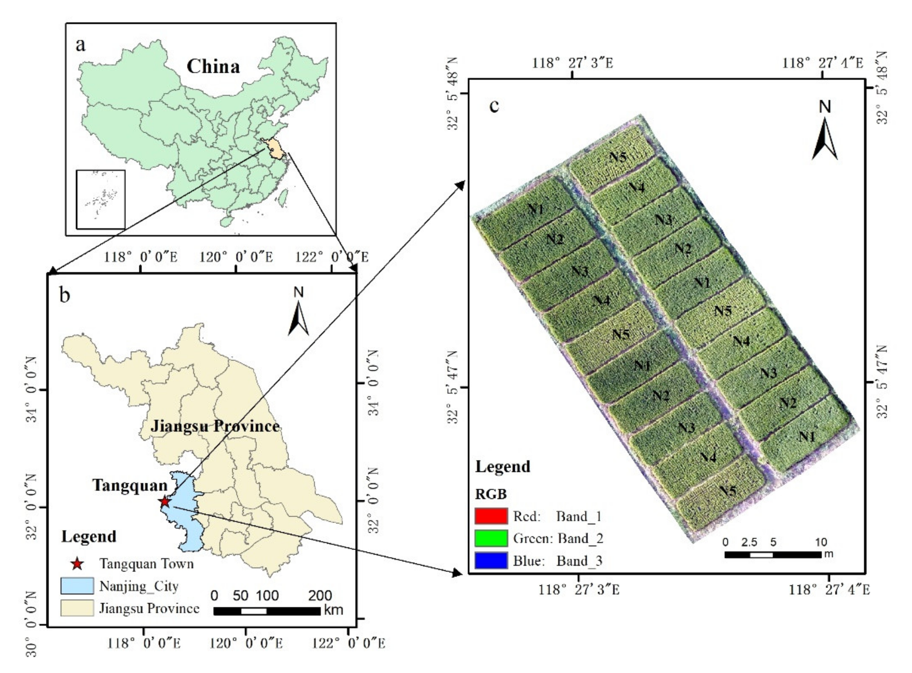
2.1. Study Area

Figure 1 shows the research area that is located in Tangquan Town, Liuhe District, Nanjing City, Jiangsu Province, China (118°27′ E, 32°05′ N, average altitude of about 36 m a.s.l.). The study area has a subtropical humid climate with four distinct seasons, and precipitation mostly occurs in summer and autumn. The average annual rainfall is 1106 mm, the annual average temperature is 15.4 °C, and the annual extreme temperature is 39.7 °C maximum and −13.1 °C minimum. The soil type in the area is paddy soil with a soil organic matter content of 22.26 g·kg⁻¹, total N of 1.31 g·kg⁻¹, Olsen-P of 15.41 mg·kg⁻¹, and NH₄OAc-K of 146.4 mg·kg⁻¹. A japonica rice cultivar with strong resistance to diseases called Nanjing 5055 in the research area was transplanted in June 12 and harvested on November 12, 2019. To increase the difference in rice growth status, five different fertilization treatments were conducted in 20 experimental plots. Each plot had an area of 40 m², and each treatment was repeated four times. The specific treatments are shown in

Table 1. Fertilization treatments in the field experiment of rice.

Fertilization Treatments	Compound Fertilizer (kg)	Urea (kg)	Controlled Release Urea (kg)	Proportion of Controlled Release N
N1	0	0	0	0
N2	3	0.4	0	0
N3	3	0.42	0.68	30%
N4	3	0.21	0.9	40%
N5	3	0	1.12	50%

and Figure 1. The planting density was 25 holes m^-2, the row spacing was 30 cm, and the planting depth was 5 cm. Other field activities were performed at normal levels.

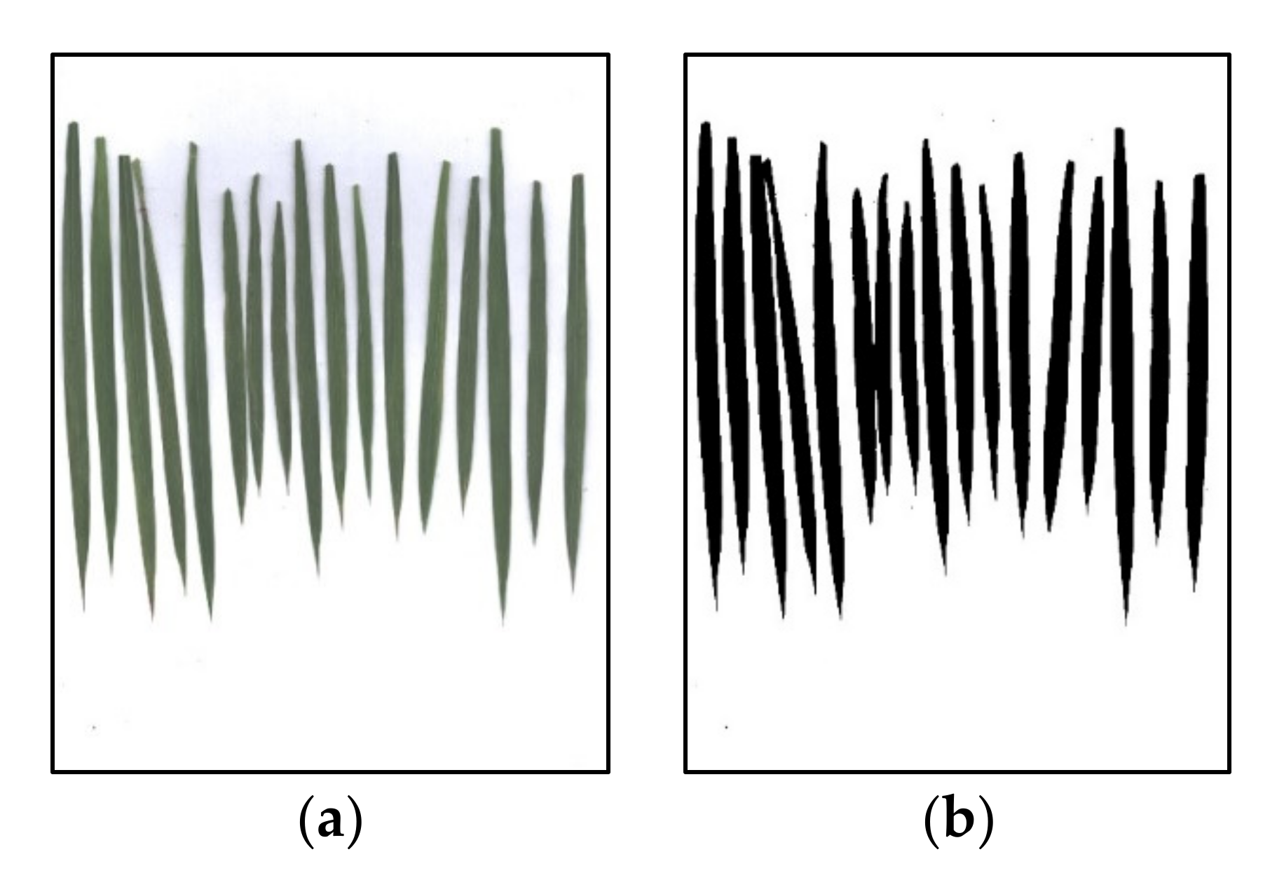
2.2. Field Data Collection

In the experiment, the key growth stage of rice was selected to collect the plant samples, as shown in

Table 2. Descriptive statistics of the growth indicators (LAI, LDB, and LTN) at different stage of rice growth.

	Date	Mean	Median	Standard Deviation	Variance	Kurtosis	Skewness	Min	Max
LAI	14 July 19	4.38	4.20	1.78	3.18	−0.32	0.31	1.33	8.10
	26 July 19	5.07	5.25	2.16	4.68	−0.70	−0.22	1.56	9.12
	12 August 19	8.68	8.99	3.51	12.29	−0.50	−0.47	2.34	14.15
	27 August 19	8.70	9.27	3.72	13.86	−1.19	−0.24	3.06	14.77
	08 September 19	7.36	7.24	2.28	5.18	−0.85	−0.23	3.37	10.76
	27 September 19	7.53	7.31	3.36	11.28	−0.76	0.19	2.33	14.09
LDB g hole−1	14 July 19	8.62	8.75	3.22	10.37	−0.23	−0.09	3.40	15.40
	26 July 19	9.72	10.00	3.52	12.42	−1.04	−0.37	3.80	14.30
	12 August 19	16.41	16.55	5.25	27.57	−0.76	−0.51	6.90	23.80
	27 August 19	17.67	17.25	6.30	39.73	−0.92	−0.05	7.60	28.90
	08 September 19	16.47	16.65	4.16	17.35	−0.42	−0.16	8.90	24.10
	27 September 19	15.10	15.75	5.11	26.14	−0.77	−0.09	6.50	23.70
LTN g kg−1	14 July 19	31.40	31.53	6.11	37.37	−0.61	−0.03	21.07	42.44
	26 July 19	29.28	30.93	6.17	38.06	−1.08	−0.23	18.77	38.93
	12 August 19	25.24	27.27	5.56	30.94	−1.42	−0.33	16.83	33.50
	27 August 19	23.26	25.47	5.08	25.81	−1.31	−0.48	14.39	29.62
	08 September 19	20.96	21.17	3.28	10.78	−0.37	−0.59	14.25	25.80
	27 September 19	17.86	19.83	5.19	26.96	−1.31	−0.36	9.34	25.01

. From each experimental plot, a representative rice plant was selected as the sample and placed in a plastic sealed bag for laboratory processing. We separated the stems and leaves of the rice plants of all samples and scanned the leaves obtained from each plot by using the BenQ M209 Pro flatbed scanner (BenQ, Inc., Taipei, Taiwan) in the laboratory. After obtaining the RGB scanned images, three LAIs of rice were calculated by binarizing the images (Figure 2). The separated leaves and stems were heated at 105 °C for 30 min and then dried at a constant temperature of 80 °C to a constant weight. The dry weights of the leaves were weighed as the leaf dry biomass (LDB) for each sample, and the total N content of the leaves was determined using the Kjeldahl method. Table 2 presents the descriptive statistics of the sampled data of the rice measurement parameters.

2.3. UAV Data Acquisition

The Phantom 4 Professional UAV (SZ DJI Technology Co., Shenzhen, China) was used to acquire the high spatial resolution images at each sampling period. The UAV was equipped with a 20-million-pixel visible light (RGB) installed in the camera. Aerial photographs of the study site were captured using the UAV flying at a height of 100 m from the ground at a speed of 8 m s^-1 (

Table 3. Data of the UAV flights and sampling dates in the corresponding rice growth stages.

Data of UAV Flights and Sampling	Growth Stage
14 July 2019	Tillering stage
26 July 2019	Early jointing stage
12 August 2019	Late jointing stage
27 August 2019	Heading stage
8 September 2019	Flowering stage
27 September 2019	Filling stage

). The side and forward overlap properties of the image were set to 60%–80%. Every flight was carried out in clear, cloudless, and windless weather. The images were captured in the joint photographic experts group (JPEG) and double-negative group (DNG) formats between 11:00 and 13:00 by a camera using auto-focus, auto-exposure time, and auto-white balance. The Pix4Dmapper (https://www.pix4d.com/) was used to generate the orthophoto images from the acquired original images. This process mainly includes importing UAV images, aligning them, constructing dense point clouds, constructing grids, generating orthophotos, generating TIFF format images with geographic coordinate systems, and performing grid division using a default parameter analysis.

2.4. UAV Image Processing and Index Extraction

We used the ENVI5.3 software (Harris Geospatial Solutions, Inc., Broomfield, CO, USA) to extract the average digital number (DN) values of the canopy red, green, and blue channels of the UAV images in each plot, denoted by R, G, and B, respectively. We then normalized the three bands (Equations (2)–(4)) through band calculation to reduce the effects of the different illumination levels.

$$r=\frac{R+G+B}{R}$$

(1)

$$\mathrm{g}=\frac{\mathrm{R}+\mathrm{G}+\mathrm{B}}{\mathrm{G}}$$

(2)

$$\mathrm{b}=\frac{\mathrm{R}+\mathrm{G}+\mathrm{B}}{\mathrm{B}}$$

(3)

where R, G, and B are the DN values of the red, green, and blue bands, respectively. Then, we used the band math tool, ENVI5.3, to perform the band operation and calculated the corresponding VI, as shown in

Table 4. List of vegetation indices (VIs) used in this study.

Name	Index	Formulation	References
Green Leaf Index	GLI	GLI = (2 × g − r + b)/(2 × g + r + b)	[40]
Green Red Vegetation Index	GRVI	GRVI = (g − r)/(g + r)	[41]
Modified Green Red Vegetation Index	MGRVI	MGRVI = (g2 − r2)/(g2 + r2)	[42]
Excess Green minus Excess Red	ExGR	ExGR = (2 × g − r − b) − (1.4 × r − g)	[21]
Excess Red Vegetation Index	ExR	ExR = 1.4 × r − g	[43]
Red Green Ratio Index	RGRI	RGRI = r/g	[44]

Note: r, g, and b represent the digital image variables of the normalized DN of R, G, and B, respectively; the same below.

. ArcGIS10.3 was used to draw the region of interest (ROI) in the center of each plot and extract the average value of various VIs at different stage in each ROI as the VI of each plot.

2.5. Image Processing

2.5.1. Optimal Index Method

Through the correlation analysis of the VIs with respect to LDB, LAI, and LTN in each growth stage, we selected the VI with the largest coefficient of determination (R²) value for each growth stage. ArcGIS10.3 was used to divide the optimal index into five levels according to the natural fault zone method. The minimum and maximum levels were removed by default, and the three middle levels were retained as the vegetation coverage area. The extracted canopy area was used to mask the original UAV images. Then, the average VI value of every ROI after masking was extracted as the VI of this plot.

2.5.2. OS Method

The OS method is based on the spectrum and texture characteristics of the UAV images [45]. First, the pixel of the rice canopy is searched as the growth point in the segmented UAV images, and then other objects in the neighborhood of the pixel are merged into the area. The newly merged area is searched and merged again until the heterogeneity of the spectrum and texture in the image is less than the preset threshold [46]. This study attempted to perform OS to extract rice canopy and noncanopy information based on rice UAV images of the key growing stage in the study area.

We used eCognition8.7, developed by Definiens (http://www.definiens.com). In eCognition, the “Scale” parameter defines the maximum standard deviation of the uniformity criteria for segmented objects. The “Shape” parameter combines objects with a characteristic shape and association with other cut blocks; it defines texture consistency. The “Compactness” parameter separates objects with relatively different shapes and uses the shape criterion and considers the total compactness to optimize the segmentation results [47]. After determining the appropriate shape, weight, and compactness, the different division scales are adjusted to ensure that the reflectivity and texture in the partitions are the same, but clear differences exist between the partitions. In this way, the canopy areas can be separated from the noncanopy areas.

2.5.3. Model Optimization

Linear, exponential, polynomial, multiple linear regression, power index, and logarithmic analyses were used to establish correlations between LDB, LAI, and LTN with UAV-Vis in the corresponding stage. We selected a correlation analysis with the largest coefficient of determination (R²) value for each rice growth indicator and each VI as the best correlation between an indicator and the index. Through comparative analysis, the VI with the largest coefficient of determination (R²) value, corresponding to different growth indicators in each growth stage, was selected as the OVI that can reflect this growth indicator during this stage. By selecting the OVI and corresponding model for the rice-monitoring indicator in each growth stage, an estimation model database was established for estimating the growth indicator throughout the growing season using UAVs.

2.5.4. Method Verification

The coefficient of determination (R²), root mean square error (RMSE), and mean absolute error (MAE) were determined to verify the reliability of the model. R² represents the fitting effect of the simulated value of the model and measured value; the closer the value is to 1, the higher is the accuracy of the model fitting. RMSE reflects the degree of dispersion between the simulated and measured values. MAE reflects the actual situation of the predicted value error. These values are calculated as follows:

$$R^2=\frac{{{\displaystyle \sum }}_{i=0}^n{\left(X_i-\overline{X}\right)}^2{\left(Y_i-Y\right)}^2}{n{{\displaystyle \sum }}_{i=0}^n{\left(X_i-X\right)}^2{{\displaystyle \sum }}_{i=0}^n{\left(Y_i-Y\right)}^2}$$

(4)

$$\mathrm{RMSE}=\sqrt{\frac{1}{\mathrm{m}}{\displaystyle \sum }_{\mathrm{i}=1}^{\mathrm{m}}{\left({\mathrm{Y}}_{\mathrm{i}}-{\mathrm{X}}_{\mathrm{i}}\right)}^2}$$

(5)

$$\mathrm{MAE}=\frac{1}{\mathrm{m}}{\displaystyle \sum }_{\mathrm{i}=1}^{\mathrm{m}}|{\mathrm{Y}}_{\mathrm{i}}-{\mathrm{X}}_{\mathrm{i}}|$$

(6)

3. Results

3.1. Correlation between Rice Growth Indicators and UAV-Based Vis at Different Growth Stages

To explore the correlation between the VI and LDB, LAI, and LTN of rice in different growth stages, the data of six key growth stages were combined to perform the correlation analysis (

Table 5. Optimized model between the key growth indicators and UAV-VI at different growth stages of rice.

Indicators	Date	Optimal VI	Optimal Model	R2
LDB	Tillering stage	GLI	y = 20.38x0.6508	0.795
	Early jointing stage	RGRI	y = 2.95x−2.4	0.853
	Late jointing stage	MGRVI	y = 39.30x1.0989	0.673
	Heading stage	MGRVI	y = 77.27x1.9317	0.871
	Flowering stage	MGRVI	y = −672.5x2 + 308.3x − 16.9	0.475
	Filling stage	ExR	y = 70.90 × 10−12.63x	0.680
LAI	Tillering stage	GLI	y = 10.24x0.6278	0.631
	Early jointing stage	MGRVI	y = 11.17x0.9598	0.752
	Late jointing stage	MGRVI	y = 28.73x1.6529	0.852
	Heading stage	GRVI	y = −1444.7x2 + 544.7x − 40.5	0.602
	Flowering stage	MGRVI	y = 22.53x0.7219	0.366
	Filling stage	ExR	y = 66.33 × 10−17.94x	0.757
LTN	Tillering stage	RGRI	y = 21.32x−0.75	0.677
	Early jointing stage	ExR	y = 0.42x−1.917	0.848
	Late jointing stage	GRVI	y = 12.11 × 102.6839x	0.719
	Heading stage	MGRVI	y = 66.94x0.9714	0.746
	Flowering stage	GRVI	y = −1468.5x2 + 384.5x − 2.3	0.668
	Filling stage	ExR	y = 314.1x2 − 282.8x + 48.6	0.915

). In most stages, except the flowering stage, the VI showed a strong correlation with the LDB, LAI, and LTN of rice. The coefficients of determination of the OVI and LDB in the key growth stages were between 0.673 and 0.871, those of the OVI and LAI were between 0.602 and 0.852, and those of the OVI and LTN were between 0.677 and 0.915. During the flowering stage, the correlation between the UAV-VI and rice growth indicators was poor.

During this stage, the rice crops showed vigorous growth; most of the VIs reached a saturated state, and the difference in rice growth indicators was small. Hence, the difference in VI performance was not clear. By establishing a simple database for estimating rice growth indicators, a reasonable estimation model could be developed for using UAV-VI to estimate the LDB, LAI, and LTN of rice at different stages.

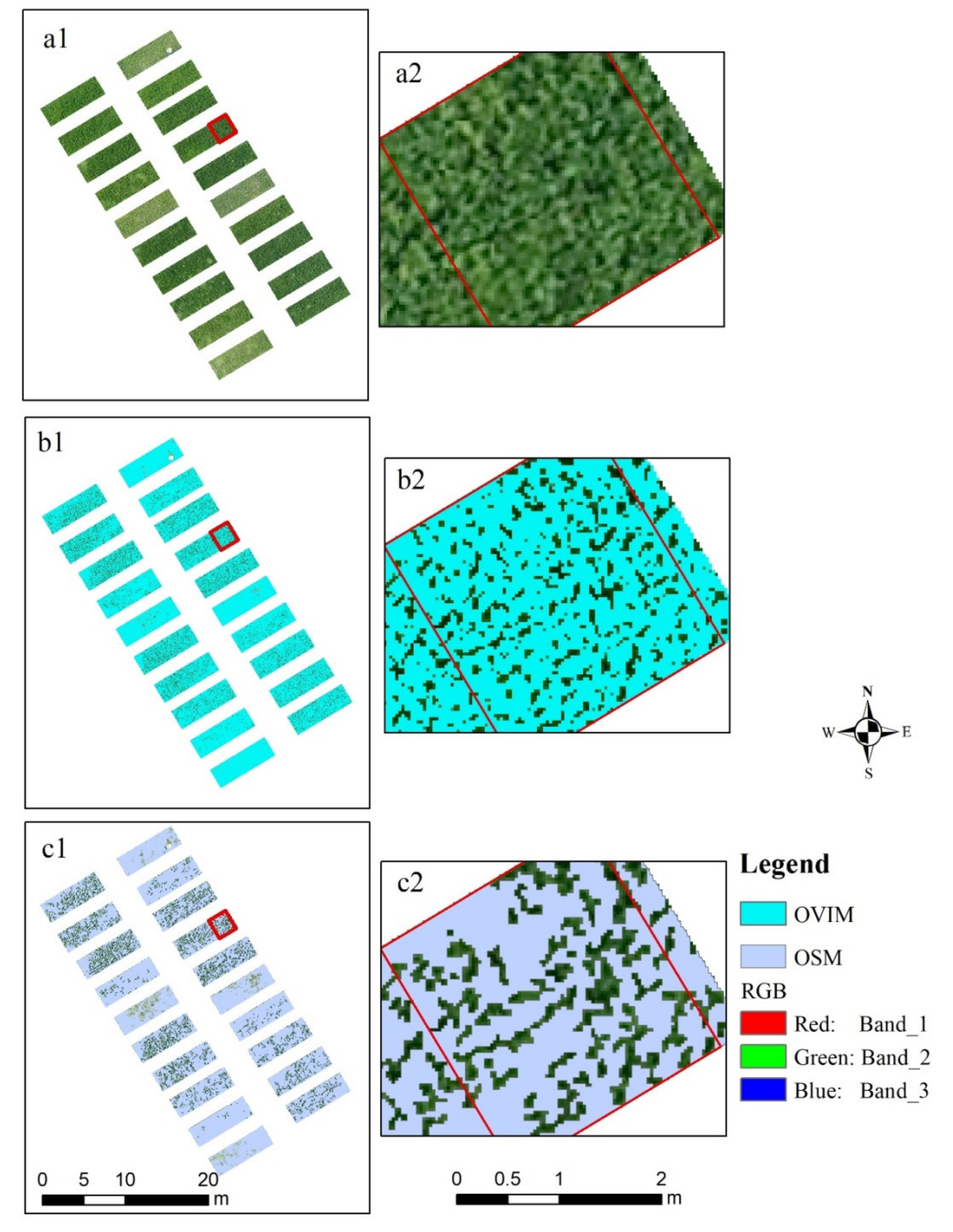
3.2. Image Noncanopy Pixel Removal

Owing to the different growth conditions of rice, the canopy coverage was different. This resulted in the appearance of noncanopy areas or the mixing of noncanopy and canopy pixels in several areas of the UAV images. To reduce the interference of noncanopy areas and mixed pixels on the UAV images, OVI and OS methods were used to process the UAV images, as shown in Figure 3; it was found that the original UAV image indicated many noncanopy pixels. The OVI method removed most of the noncanopy interference of the image (Figure 3b1,b2), and Figure 3c1,c2 showed the results using the OS method; when the black background color was removed, some mixed and canopy pixels were also removed.

3.3. Estimation Model of Key Growth Indicators and OVI Using Different Methods

During the rice growth stage, we used the OVI and OS methods to remove noncanopy pixel interference from the UAV images of each key growth stage and then re-established the relationship between the UAV-VI and the monitoring indicators. The results of the models and coefficient of determination are shown in Table 5.

Table 6. Estimation model and accuracy comparison of key growth indicators and the optimal index under different methods.

			No Processing		Optimal Index Method		Object-Oriented Segmentation Method
	Date	UAV-VI	Model 1	R2	Model 2	R2	Model 3	R2
	Tillering stage	GLI	y = 20.38x0.6508	0.795	y = 31.37x0.9823	0.818	y = 24.40x0.7844	0.829
	Early jointing stage	RGRI	y = 2.95x−2.4	0.853	y = 2.55x−2.842	0.881	y = 2.83x−2.494	0.876
	Late jointing stage	MGRVI	y = 39.30x1.0989	0.673	y = 49.13x1.279	0.687	y = 51.73x1.357	0.702
LDB	Heading stage	RGRI	y = − 1482.3x2 + 2081.2x − 709.0	0.588	y = − 2412.5x2 + 3497.7x − 1246.6	0.648	y = − 2186.1x2 + 3150.6x − 1114.3	0.626
	Flowering stage	MGRVI	y = − 672.55x2 + 308.3x − 16.9	0.475	y = − 913.2x2 + 386.2x − 22.8	0.510	y = − 1138.1x2 + 486.8x − 33.6	0.552
	Filling stage	ExR	y = 70.90 × 10−12.63x	0.680	y = 90.667 × 10−14.45x	0.747	y = 101.20 × 10−15.16x	0.755
	Tillering stage	GLI	y = 10.24x0.6278	0.631	y = 15.10x0.9435	0.688	y = 11.67x0.7425	0.677
	Early jointing stage	MGRVI	y = 11.17x0.9598	0.752	y = 13.33x1.1497	0.803	y = 11.54x1.0217	0.790
	Late jointing stage	MGRVI	y = 28.73x1.6529	0.852	y = 40.55x1.9319	0.868	y = 43.35x2.0367	0.875
LAI	Heading stage	GRVI	y = − 1444.7x2 + 544.7x − 40.5	0.602	y = − 2056.8x2 + 709.4x − 51.0	0.688	y = − 1762.3x2 + 626.8x − 45.6	0.697
	Flowering stage	MGRVI	y = 22.53x0.7219	0.366	y = 30.83x0.8767	0.433	y = 29.65x0.8765	0.422
	Filling stage	ExR	y = 66.33 × 10−17.94x	0.757	y = 95.01 × 10−20.59x	0.818	y = 100.3 × 10−20.93x	0.777
	Tillering stage	RGRI	y = 21.319x−0.75	0.677	y = 20.051x−0.865	0.704	y = 20.80x−0.795	0.704
	Early jointing stage	ExR	y = 0.42x−1.917	0.848	y = 0.27x−2.135	0.857	y = 0.44x−1.9	0.861
	Late jointing stage	GRVI	y = 12.11 × 102.6839x	0.719	y = 10.59 × 103.618x	0.737	y = 10.32 × 103.6643x	0.735
LTN	Heading stage	MGRVI	y = 66.94x0.9714	0.746	y = 214.8x1.2114	0.800	y = 204.1x1.1947	0.799
	Flowering stage	GRVI	y = − 1468.5x2 + 384.5x − 2.3	0.668	y = − 1570.0x2 + 400.3x − 2.60	0.717	y = − 2480.6x2 + 584.8x − 11.6	0.720
	Filling stage	ExR	y = 314.05x2 − 282.8x + 48.6	0.915	y = 464.6x2 − 341.1x + 53.8	0.930	y = 904.9x2 − 470.6x + 63.2	0.931

shows that the coefficient of determination between the monitoring indicators and the VI was improved to various degrees after processing the noncanopy pixels of the UAV images using the two methods. When the correlation coefficient between the VI and monitoring indicators was small, the increase in the coefficient of determination was large after processing in the case of both the methods. In contrast, when the coefficient of determination was small, the increase in the coefficient of determination was small after processing in the case of both the methods.

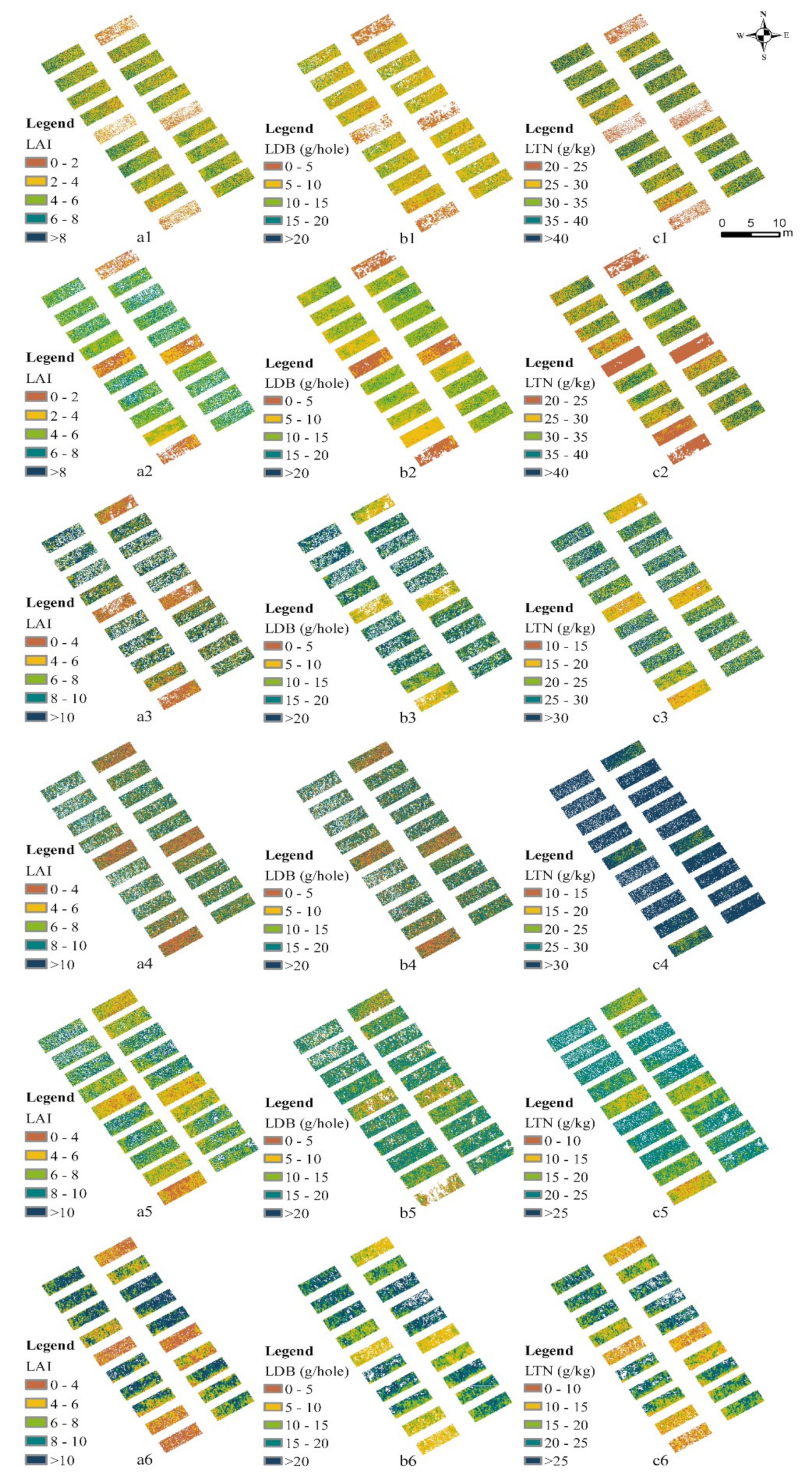
3.4. Estimation Results of Rice Growth Indicators Using a Simple Model Database

By using the OVI and OS methods to remove the noncanopy pixels, the estimation accuracy was improved to a certain extent. We selected the model with the best correlation of each rice growth indicator in each growth stage to establish a simple estimation model database (Table 6), which could be used as a guide to monitor the rice growth status through UAVs. The model database showed that, except for the flowering stage at which the coefficients of determination of LDB and LAI were 0.552 and 0.433, respectively, the coefficients of all models in all other stages were greater than 0.60, indicating that the model in this database could be used to estimate the key growth indicators of rice at different stages. Meanwhile, we estimated the LAI, LDB, and LTN in the six growing stages of rice by using the model in the database (Figure 4), and different monitoring indicators of rice differed for different fertilization treatments. In the nonfertilized plots, the values of the monitoring indicators were smaller. In the plots with N fertilization, the key monitoring indicators of rice were larger than those for plots without fertilization. In the plots without N-controlled fertilizations, the important monitoring indicators of rice were worse than the application of N-containing controlled-release fertilizer, which showed that the N-containing controlled-release fertilizers had a greater effect on rice growth.

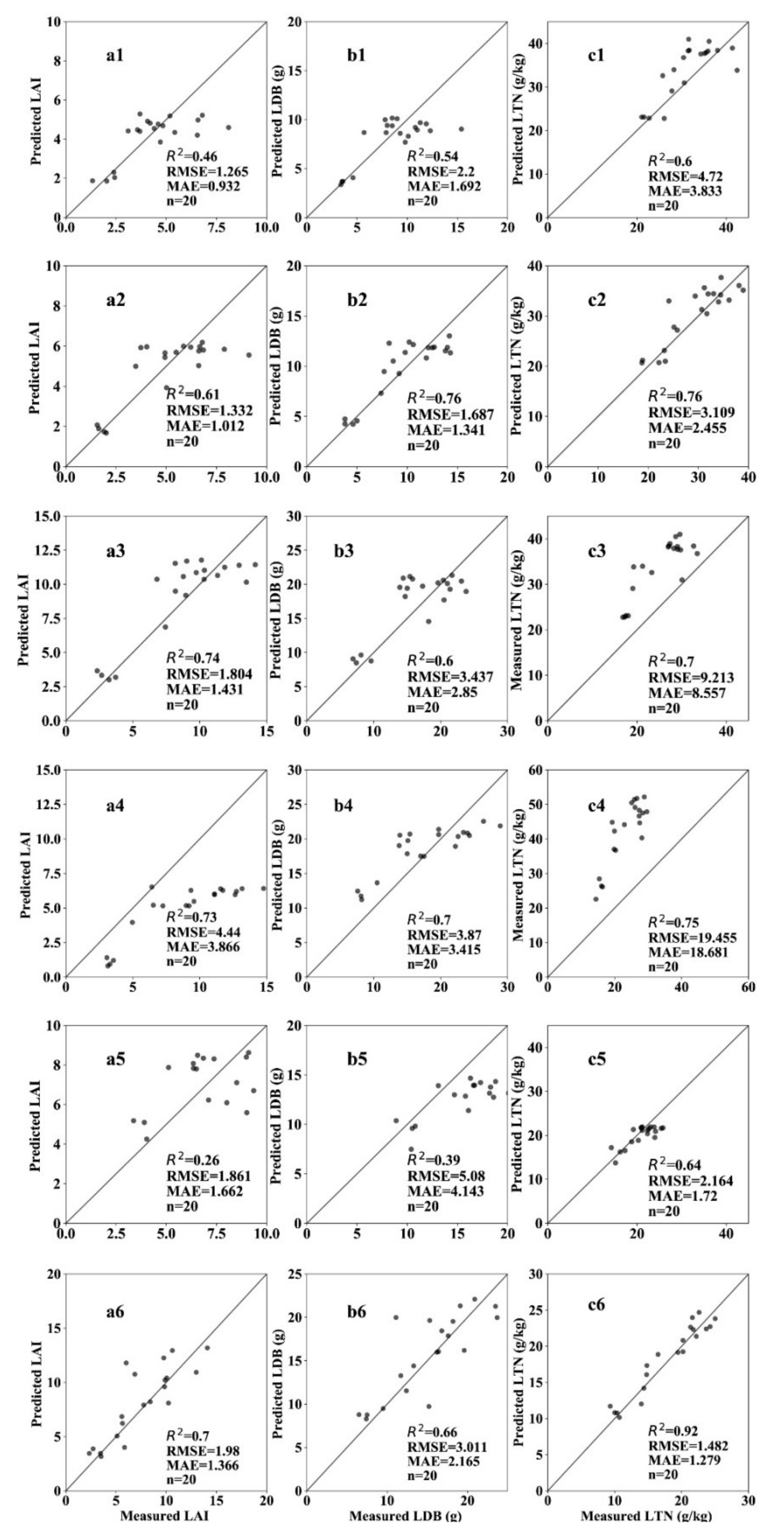
3.5. Validation of Estimation Results of Key Growth Indicators in Different Growth Stages

Figure 5 shows the verification of the estimation results of the key growth indicators at different growth stages using this simple database. At the tillering stage, the verification accuracy of the LAI, LDB, and LTN were 0.46, 0.54, and 0.60, respectively, and the RMSE values were 1.265, 2.2, and 4.72, respectively. At the jointing stage, the verification accuracy of the three indicators ranged from 0.6 to 0.8. This indicated that the estimation result in the jointing stage was better than that in the tillering stage. At the booting stage, the estimated verification accuracies of the three key growth indicators were between 0.7 and 0.8, and their corresponding RMSE values were 4.44, 3.87, and 19.455, respectively, and the MAE values were 3.866, 3.415, and 18.68, respectively. Although the verification accuracy of the booting stage was higher than that of the jointing stage, the RMSE and MAE were all too large, which implied that the error between the estimation results and actual observations at the booting stage was greater than that at the jointing stage. At the flowering stage, the verification accuracies of the estimation of LAI and LDB were 0.26 and 0.39, respectively. This might be because the rice grew vigorously during this stage, and the difference in the UAV imagery was not evident. The verification accuracy of the LTN estimation was 0.64, indicating a better estimation accuracy of this indicator than those of the LAI and LDB at this growth stage. At the filling stage, the verification accuracy of the LAI, LDB, and LTN estimation increased, with an RMSE of 1.980, 3.011, and 1.482 and MAE of 1.366, 2.165, and 1.279, respectively. The verification accuracy of the LTN estimation was as high as 0.92, indicating that the UAV-VI was used to estimate the LTN with the highest accuracy during the filling stage. In general, it was feasible to use a simple model with the model database to estimate the key growth indicators of rice, and some differences were observed in the estimation accuracy at the different stages.

4. Discussion

4.1. Simple Model Database for Estimating Rice Growth Indicators

Many studies have used UAVs to monitor crop growth indicators, focusing on monitoring a single indicator at a certain stage [22,38,44]. By analyzing the correlation between the UAV-VI and rice growth indicators at each growth stage, a simple model database was established for estimating the rice growth indicators. A reasonable estimation model was established for using UAV-VI to estimate the rice LDB, LAI, and LTN at the different stages. This study used the red, green, and blue bands included in the digital camera of Phantom 4 Professional. The VIs extracted from the UAV images are GLI, GRVI, MGRVI, ExGR, ExR, and RGRI [2,44], which have been widely used in crop monitoring. Many indicators reflect the growth status of crops. In this study, the canopy indicators, LDB, LAI, and LTN, were considered, which were easily monitored by UAV and showed good correlation with crop yields. Therefore, the use of UAVs to rapidly monitor rice growth status and diagnose nutritional indicators was crucial for precise management of crop monitoring. The simple estimation model database established in this study provided guidance and suggestions for monitoring the growth status of rice using UAVs. In different growth stages, farmers can use the model in the database to estimate the crop growth index. In this study, a simple estimation model database was developed based on the Tangquan experimental field; the rice variety was japonica rice, a cultivar called Nanjing 5055, and the result could be applied around Nanjing using similar rice varieties. In the actual monitoring process, the monitoring results may differ due to the different rice varieties and monitoring scales. Therefore, in future research, for improving the estimation accuracy of the rice varieties, the monitoring scales should be extended in the model database.

4.2. Feasibility of Monitoring Rice Growth Indicators Using Uavs

To monitor the crop growth indicators, several researchers have used UAVs equipped with hyperspectral cameras, multispectral cameras, and lidars [14,45,46,47]. Although such monitoring reflected the growth status of the vegetation, it was not easy to popularize and apply due to its high cost. By using the images in different growing seasons of rice captured from the DJI RGB camera, the corresponding VIs could be used to estimate the rice growth indicators; this method is not only easy to analyze and apply to the field of rice growth, but also it can reduce costs and display the growth of rice rapidly and accurately, hence providing guidance and suggestions for field management.

UAV was used in this study to monitor multiple growth indicators of rice at different stages, but it only met the monitoring of rice indicators at a small scale due to the limitation of flight time. Although the monitoring area by UAVs is small at a time, it has the advantages of high spatial resolution, strong timeliness, and less influence of weather, which is enough to ensure accurate guidance for agricultural management. If it needs to be applied to large areas, satellite remote sensing images need to be used for monitoring. However, satellite images have the disadvantages of a lower spatial resolution than that of UAV images and are easily influenced by weather changes, and it is often difficult to meet precision agricultural guidance at the plot level.

4.3. Different Methods to Remove Noncanopy Pixels

The use of the OVI method could remove areas with particularly critical effects of noncanopy areas on the VI [48], and areas with less impact were not completely removed. The OS method used the texture and spectral features of the UAV image for segmentation so that the heterogeneity of the spectrum and texture in the same segmentation area was small, while that in the different segmentation areas was large [49,50]. However, although the two methods of removing noncanopy pixels could improve the estimation accuracy, both methods showed certain flaws. The OVI method demonstrated different indexes in different plots, and therefore the precise index threshold was difficult to determine, and the method could remove most of the noncanopy area, while a small amount of noncanopy area was difficult to remove. In the case of the OS method, owing to the homogeneity and heterogeneity of the segmentation process [51], part of the vegetation canopy was also removed, thus reducing the stability of the method.

5. Conclusions

In this study, consumer UAVs were used to establish estimation models for the key growth indicators of rice at different growth stages based on seven VIs obtained through UAVs. We also used the OVI and OS methods to remove the noncanopy pixels from the image. The use of the OVI and OS methods can remove part of the noncanopy area, which can improve the correlation between each growth indicator and the VIs. Furthermore, a sample estimation model database was created and was used to estimate the LAI, LDB, and LTN indicators of rice at different growth stages, and the model in this database can be used to estimate the key growth indicators of rice at different stages. The application of this model database offered a new idea for the better use of UAVs for monitoring rice growth conditions and guiding precision rice management. Future work should focus on the estimating accuracy regarding the different rice varieties and monitoring scales in the model database.

References

1. Li, P.; Zhang, X.; Wang, W.; Zheng, H.; Yao, X.; Tian, Y.; Zhu, Y.; Cao, W.; Chen, Q.; Cheng, T. Estimating aboveground and organ biomass of plant canopies across the entire season of rice growth with terrestrial laser scanning. Int. J. Appl. Earth Obs. Geoinf. 2020, 91, 102–132. [Google Scholar] [CrossRef]
2. Yang, B.; Wang, M.; Sha, Z.; Wang, B.; Chen, J.; Yao, X.; Cheng, T.; Cao, W.; Zhu, Y. Evaluation of aboveground nitrogen content of winter wheat using digital imagery of unmanned aerial vehicles. Sensors 2019, 19, 4416. [Google Scholar] [CrossRef] [PubMed] [Green Version]
3. Zhang, N.; Wang, M.; Wang, N. Precision agriculture—A worldwide overview. Comput. Electron. Agric. 2002, 36, 113–132. [Google Scholar] [CrossRef]
4. Qiu, Z.; Liu, H.; Zhang, X.; Meng, L.; Xu, M.; Pan, Y.; Bao, Y.; Yu, S. Analysis of spatiotemporal variation of site-specific management zones in a topographic relief area over a period of six years using image segmentation and satellite data. Can. J. Remote Sens. 2019, 45, 746–758. [Google Scholar] [CrossRef]
5. Xu, X.; Teng, C.; Zhao, Y.; Du, Y.; Zhao, C.; Yang, G.; Jin, X.; Song, X.; Gu, X.; Casa, R.; et al. Prediction of wheat grain protein by coupling multisource remote sensing imagery and ECMWF data. Remote Sens. 2020, 12, 1349. [Google Scholar] [CrossRef]
6. Canisius, F.; Fernandes, R. ALOS PALSAR L-band polarimetric SAR data and in situ measurements for leaf area index assessment. Remote Sens. Lett. 2012, 3, 221–229. [Google Scholar] [CrossRef]
7. Gahrouei, O.R.; McNairn, H.; Hosseini, M.; Homayouni, S. Estimation of crop biomass and leaf area index from multitemporal and multispectral imagery using machine learning approaches. Can. J. Remote Sens. 2020, 46, 1712–7971. [Google Scholar] [CrossRef]
8. Li, W.; Niu, Z.; Wang, C.; Huang, W.; Chen, H.; Gao, S.; Li, D.; Muhammad, S. Combined use of airborne LiDAR and satellite gf-1 data to estimate leaf area index, height, and aboveground biomass of maize during peak growing season. IEEE J. Sel. Top. Appl. Earth Obs. Remote Sens. 2015, 8, 4489–4501. [Google Scholar] [CrossRef]
9. Tsui, O.W.; Coops, N.C.; Wulder, M.A.; Marshall, P.L.; McCardle, A. Using multi-frequency radar and discrete-return LiDAR measurements to estimate above-ground biomass and biomass components in a coastal temperate forest. ISPRS J. Photogramm. Remote Sens. 2012, 69, 121–133. [Google Scholar] [CrossRef]
10. Zhu, X.; Liu, D. Improving forest aboveground biomass estimation using seasonal Landsat NDVI time-series. ISPRS J. Photogramm. Remote Sens. 2015, 102, 222–231. [Google Scholar] [CrossRef]
11. Battude, M.; Al Bitar, A.; Morin, D.; Cros, J.; Huc, M.; Marais Sicre, C.; Le Dantec, V.; Demarez, V. Estimating maize biomass and yield over large areas using high spatial and temporal resolution Sentinel-2 like remote sensing data. Remote Sens. Environ. 2016, 184, 668–681. [Google Scholar] [CrossRef]
12. Duan, T.; Chapman, S.C.; Guo, Y.; Zheng, B. Dynamic monitoring of NDVI in wheat agronomy and breeding trials using an unmanned aerial vehicle. Field Crop. Res. 2017, 210, 71–80. [Google Scholar] [CrossRef]
13. Li, S.; Ding, X.; Kuang, Q.; Ata-Ui-Karim, S.T.; Cheng, T.; Liu, X.; Tian, Y.; Zhu, Y.; Cao, W.; Cao, Q. Potential of UAV-based active sensing for monitoring rice leaf nitrogen status. Front Plant Sci. 2018, 9, 1834. [Google Scholar] [CrossRef] [PubMed] [Green Version]
14. Lu, N.; Wang, W.; Zhang, Q.; Li, D.; Yao, X.; Tian, Y.; Zhu, Y.; Cao, W.; Baret, F.; Liu, S.; et al. Estimation of nitrogen nutrition status in winter wheat from unmanned aerial vehicle based multi-angular multispectral imagery. Front Plant Sci. 2019, 10, 1601. [Google Scholar] [CrossRef] [Green Version]
15. Zheng, H.; Cheng, T.; Li, D.; Yao, X.; Tian, Y.; Cao, W.; Zhu, Y. Combining unmanned aerial vehicle (UAV)-based multispectral imagery and ground-based hyperspectral data for plant nitrogen concentration estimation in rice. Front Plant Sci. 2018, 9, 936. [Google Scholar] [CrossRef]
16. Zheng, H.; Li, W.; Jiang, J.; Liu, Y.; Cheng, T.; Tian, Y.; Zhu, Y.; Cao, W.; Zhang, Y.; Yao, X. A comparative assessment of different modeling algorithms for estimating leaf nitrogen content in winter wheat using multispectral images from an unmanned aerial vehicle. Remote Sens. 2018, 10, 2026. [Google Scholar] [CrossRef] [Green Version]
17. Herrmann, I.; Bdolach, E.; Montekyo, Y.; Rachmilevitch, S.; Townsend, P.A.; Karnieli, A. Assessment of maize yield and phenology by drone-mounted superspectral camera. Precis. Agric. 2020, 21, 51–76. [Google Scholar] [CrossRef]
18. Zhou, X.; Zheng, H.B.; Xu, X.Q.; He, J.Y.; Ge, X.K.; Yao, X.; Cheng, T.; Zhu, Y.; Cao, W.X.; Tian, Y.C. Predicting grain yield in rice using multi-temporal vegetation indices from UAV-based multispectral and digital imagery. ISPRS J. Photogramm. Remote Sens. 2017, 130, 246–255. [Google Scholar] [CrossRef]
19. Zheng, H.; Cheng, T.; Zhou, M.; Li, D.; Yao, X.; Tian, Y.; Cao, W.; Zhu, Y. Improved estimation of rice aboveground biomass combining textural and spectral analysis of UAV imagery. Precis. Agric. 2018, 20, 611–629. [Google Scholar] [CrossRef]
20. Lu, N.; Zhou, J.; Han, Z.; Li, D.; Cao, Q.; Yao, X.; Tian, Y.; Zhu, Y.; Cao, W.; Cheng, T. Improved estimation of aboveground biomass in wheat from RGB imagery and point cloud data acquired with a low-cost unmanned aerial vehicle system. Plant Methods 2019, 15, 17. [Google Scholar] [CrossRef] [Green Version]
21. Tilly, N.; Aasen, H.; Bareth, G. Fusion of plant height and vegeta-tion indices for the estimation of barley biomass. Remote Sens. 2015, 7, 11449–11480. [Google Scholar] [CrossRef] [Green Version]
22. Li, W.; Niu, Z.; Chen, H.; Li, D.; Wu, M.; Zhao, W. Remote estimation of canopy height and aboveground biomass of maize using high-resolution stereo images from a low-cost unmanned aerial vehicle system. Ecol. Indic. 2016, 67, 637–648. [Google Scholar] [CrossRef]
23. Han, L.; Yang, G.; Dai, H.; Yang, H.; Xu, B.; Feng, H.; Li, Z.H.; Yang, X. Fuzzy clustering of maize plant-height patterns using time series of UAV remote-sensing images and variety traits. Front. Plant Sci. 2019, 10, 926. [Google Scholar] [CrossRef] [PubMed] [Green Version]
24. Han, L.; Yang, G.; Dai, H.; Xu, B.; Yang, H.; Feng, H.; Li, Z.H.; Yang, X.D. Modeling maize above-ground biomass based on machine learning approaches using UAV remote-sensing data. Plant Methods 2019, 15, 10. [Google Scholar] [CrossRef] [PubMed] [Green Version]
25. Liang, W.; Cen, H.; Zhu, J.; Zhang, J.; Zhu, Y.; Sun, D.; Du, X.; Zhai, L.; Weng, H.; Li, Y.; et al. Grain yield prediction of rice using multi-temporal UAV-based RGB and multispectral images and model transfer a case study of small farmlands in the south of China. Agric. For. Meteorol. 2020, 291, 108096. [Google Scholar]
26. Wang, W.; Yao, X.; Yao, X.F.; Tian, Y.C.; Liu, X.J.; Ni, J.; Cao, W.X.; Zhu, Y. Estimating leaf nitrogen concentration with three-band vegetation indices in rice and wheat. Field Crop. Res. 2012, 129, 90–98. [Google Scholar] [CrossRef]
27. Zha, H.; Miao, Y.; Wang, T.; Li, Y.; Zhang, J.; Sun, W.; Feng, Z.; Kusnierek, K. Improving unmanned aerial vehicle remote sensing-based rice nitrogen nutrition index prediction with machine learning. Remote Sens. 2020, 12, 215. [Google Scholar] [CrossRef] [Green Version]
28. Li, B.; Xu, X.; Zhang, L.; Han, J.; Bian, C.; Li, G.; Liu, J.; Jin, L. Above-ground biomass estimation and yield prediction in potato by using UAV-based RGB and hyperspectral imaging. ISPRS J. Photogramm. Remote Sens. 2020, 162, 161–172. [Google Scholar] [CrossRef]
29. Zheng, H.; Cheng, T.; Li, D.; Zhou, X.; Yao, X.; Tian, Y.; Cao, W.; Zhu, Y. Evaluation of RGB, color-infrared and multispectral images acquired from unmanned aerial systems for the estimation of nitrogen accumulation in rice. Remote Sens. 2018, 10, 824. [Google Scholar] [CrossRef] [Green Version]
30. Wang, Y.; Wang, D.; Zhang, G.; Wang, J. Estimating nitrogen status of rice using the image segmentation of G-R thresholding method. Field Crop. Res. 2013, 149, 33–39. [Google Scholar] [CrossRef]
31. Mohan, M.; Silva, C.; Klauberg, C.; Jat, P.; Catts, G.; Cardil, A.; Hudak, A.; Dia, M. Individual tree detection from unmanned aerial vehicle (UAV) derived canopy height model in an open canopy mixed conifer forest. Forests 2017, 8, 340. [Google Scholar] [CrossRef] [Green Version]
32. Zhou, C.; Ye, H.; Xu, Z.; Hu, J.; Shi, X.; Hua, S.; Yue, J.; Yang, G. Estimating maize-leaf coverage in field conditions by applying a machine learning algorithm to UAV remote sensing images. Appl. Sci. 2019, 9, 2389. [Google Scholar] [CrossRef] [Green Version]
33. Pekkarinen, A. A method for the segmentation of very high spatial resolution images of forested landscapes. Int. J. Remote Sens. 2002, 23, 2817–2836. [Google Scholar] [CrossRef]
34. Schiewe, J. Integration of multi-sensor data for landscape modeling using a region-based approach. ISPRS J. Photogramm. Remote Sens. 2003, 57, 371–379. [Google Scholar] [CrossRef]
35. Stow, D.; Lopez, A.; Lippitt, C.; Hinton, S.; Weeks, J. Object-based classification of residential land use within Accra, Ghana based on QuickBird satellite data. Int. J. Remote Sens. 2007, 28, 5167–5173. [Google Scholar] [CrossRef] [PubMed]
36. Gamanya, R.; De Maeyer, P.; De Dapper, M. Object-oriented change detection for the city of Harare, Zimbabwe. Expert Syst. Appl. 2009, 36, 571–588. [Google Scholar] [CrossRef]
37. Liu, H.J.; Whiting, M.L.; Ustin, S.L.; Zarco-Tejada, P.J.; Huffman, T.; Zhang, X.L. Maximizing the relationship of yield to site-specific management zones with object-oriented segmentation of hyperspectral images. Precis. Agric. 2018, 19, 348–364. [Google Scholar] [CrossRef] [Green Version]
38. Martha, T.R.; Kerle, N.; Jetten, V.; van Westen, C.J.; Kumar, K.V. Characterizing spectral, spatial and morphometric properties of landslides for semi-automatic detection using object-oriented methods. Geomorphology 2010, 116, 24–36. [Google Scholar] [CrossRef]
39. Tong, Q.; Shan, J.; Zhu, B.; Ge, X.; Sun, X.; Liu, Z. Object-oriented coastline classification and extraction from remote sensing imagery. In Remote Sensing of the Environment: 18th National Symposium on Remote Sensing of China, Wuhan, China, 20–23 October 2012; International Society for Optics and Photonics: Bellingham, WA, USA, 2014. [Google Scholar]
40. Louhaichi, M.; Borman, M.M.; Johnson, D.E. Spatially located platform and aerial photography for documentation of grazing impacts on wheat. Geocarto Int. 2008, 16, 65–70. [Google Scholar] [CrossRef]
41. Tucker, C.J. Red and photographic infrared linear combinations for monitoring vegetation. Remote Sens. Environ. 1979, 8, 127–150. [Google Scholar] [CrossRef] [Green Version]
42. Bendig, J.; Yu, K.; Aasen, H.; Bolten, A.; Bennertz, S.; Broscheit, J.; Gnyp, M.L.; Bareth, G. Combining UAV-based plant height from crop surface models, visible, and near infrared vegetation indices for biomass monitoring in barley. Int. J. Appl. Earth Obs. Geoinf. 2015, 39, 79–87. [Google Scholar] [CrossRef]
43. Meyer, G.E.; Neto, J.C. Verification of color vegetation indices for automated crop imaging applications. Comput. Electron. Agric. 2008, 63, 282–293. [Google Scholar] [CrossRef]
44. Verrelst, J.; Schaepman, M.E.; Koetz, B.; Kneubühler, M. Angular sensitivity analysis of vegetation indices derived from CHRIS/PROBA data. Remote Sens. Environ. 2008, 112, 2341–2353. [Google Scholar] [CrossRef]
45. Bo, L.; Jian, C. Segmentation algorithm of high resolution remote sensing images based on LBP and statistical region merging. In Proceedings of the 2012 International Conference on Audio, Language, and Image Processing, Shanghai, China, 16–18 July 2012; Institute of Electrical and Electronics Engineers: Piscataway, NJ, USA, 2012. [Google Scholar]
46. Benz, U.C.; Hofmann, P.; Willhauck, G.; Lingenfelder, I.; Heynen, M. Multi-resolution, object-oriented fuzzy analysis of remote sensing data for GIS-ready information. ISPRS J. Photogramm. Remote Sens. 2004, 58, 239–258. [Google Scholar] [CrossRef]
47. Frohn, R.C.; Autrey, B.C.; Lane, C.R.; Reif, M. Segmentation and object-oriented classification of wetlands in a karst Florida landscape using multi-season Landsat-7 ETM+ imagery. Int. J. Remote Sens. 2011, 32, 1471–1489. [Google Scholar] [CrossRef]
48. Woebbecke, D.M.; Meyer, G.E.; Bargen, K.V.; Mortensen, D.A. Color indices for weed identification under various soil, residue, and lighting conditions. Trans. ASAE 1995, 38, 259–269. [Google Scholar] [CrossRef]
49. Gamanya, R.; Maeyer, P.D.; Dapper, M.D. An automated satellite image classification design using object-oriented segmentation algorithms: A move towards standardization. Expert Syst. Appl. 2007, 32, 616–624. [Google Scholar] [CrossRef]
50. Dhawan, A.P. Image segmentation and feature extraction. In Principles and Advanced Methods in Medical Imaging and Image Analysis; World Scientific Publishing Company: Singapore, 2015. [Google Scholar]
51. Wang, Y.; Qi, Q.; Jiang, L.; Liu, Y. Hybrid remote sensing image segmentation considering intersegment homogeneity and intersegment heterogeneity. IEEE Geosci. Remote Sens. Lett. 2019, 17, 1–5. [Google Scholar] [CrossRef]
Figure 1. Geographic location of the research area and a UAV image of the experimental plots with 5 fertilization treatments ((a), the location of Jiangsu Province in China; (b), the location of Nanjing City in Jiangsu Province and the location of Tangquan Town in Nanjing City; (c), a UAV image of the experimental plots).
Remotesensing 12 03228 g001
Figure 2. (a) Scanned image of the leaves; and (b) the binarized image results of the scanned image.
Remotesensing 12 03228 g002
Figure 3. The results of noncanopy pixel removal of UAV images. (a1,a2: original UAV images; b1,b2: the process of OVI method; and c1,c2: the process of OS method; a2,b2,c2 are the magnified results of a certain area in a1,b1,c1, respectively).
Remotesensing 12 03228 g003
Figure 4. Estimated maps of the key monitoring indicators at different growth stage. LAI, LDB, and LTN at the tillering stage (a1,b1,c1), early jointing stage (a2,b2,c2), late jointing stage (a3,b3,c3), heading stage (a4,b4,c4), flowering stage (a5,b5,c5), and filling stage (a6,b6,c6).
Remotesensing 12 03228 g004
Figure 5. Verification of the estimation results of the key growth indicators at different growth stages. LAI, LDB, and LTN at the tillering stage (a1,b1,c1), early jointing stage (a2,b2,c2), late jointing stage (a3,b3,c3), heading stage (a4,b4,c4), flowering stage (a5,b5,c5), and filling stage (a6,b6,c6).
Remotesensing 12 03228 g005