Article

Evaluating Forest Cover and Fragmentation in Costa Rica with a Corrected Global Tree Cover Map

Department of Geography and Environmental Systems, University of Maryland, Baltimore County, Baltimore, MD 21250, USA
*
Author to whom correspondence should be addressed.
Remote Sens. 2020, 12(19), 3226; https://doi.org/10.3390/rs12193226
Submission received: 26 June 2020 / Revised: 12 September 2020 / Accepted: 27 September 2020 / Published: 3 October 2020
(This article belongs to the Special Issue Global Biospheric Monitoring with Remote Sensing)

Abstract

:
Global tree cover products face challenges in accurately predicting tree cover across biophysical gradients, such as precipitation or agricultural cover. To generate a natural forest cover map for Costa Rica, biases in tree cover estimation in the most widely used tree cover product (the Global Forest Change product (GFC) were quantified and corrected, and the impact of map biases on estimates of forest cover and fragmentation was examined. First, a forest reference dataset was developed to examine how the difference between reference and GFC-predicted tree cover estimates varied along gradients of precipitation and elevation, and nonlinear statistical models were fit to predict the bias. Next, an agricultural land cover map was generated by classifying Landsat and ALOS PalSAR imagery (overall accuracy of 97%) to allow removing six common agricultural crops from estimates of tree cover. Finally, the GFC product was corrected through an integrated process using the nonlinear predictions of precipitation and elevation biases and the agricultural crop map as inputs. The accuracy of tree cover prediction increased by ≈29% over the original global forest change product (the R2 rose from 0.416 to 0.538). Using an optimized 89% tree cover threshold to create a forest/nonforest map, we found that fragmentation declined and core forest area and connectivity increased in the corrected forest cover map, especially in dry tropical forests, protected areas, and designated habitat corridors. By contrast, the core forest area decreased locally where agricultural fields were removed from estimates of natural tree cover. This research demonstrates a simple, transferable methodology to correct for observed biases in the Global Forest Change product. The use of uncorrected tree cover products may markedly over- or underestimate forest cover and fragmentation, especially in tropical regions with low precipitation, significant topography, and/or perennial agricultural production.

1. Introduction

Recent deforestation across the tropics has resulted in extensive habitat loss, carbon emissions, and species extinctions [1,2,3,4]. Although these trends are projected to intensify in the near term [1,5,6], quantifying pantropical deforestation rates remains challenging [7]. National deforestation estimates are often debated [8,9,10], especially when estimates informed by field plots differ from those derived from remote sensing imagery [11]. Global maps of forest cover derived from remote sensing can assist with estimates of loss across the tropics, but challenges remain in generating consistent forest cover estimates [7,12]. These challenges include high wet season cloud cover, broad phenological differences across tropical forests, persistent confusion between forests and perennial crops, and a diversity of national definitions of “forest”, which varies in its structure and cover across ecosystems and cultures [13,14,15]. Maps of tropical forests must encompass variability along numerous abiotic and biotic gradients. Forest structure and reflectance across tropical regions vary in response to topography [16], cloud cover [17,18], precipitation [19], phenological variability [20], and the presence of perennial erect crops (“tree crops”) that resemble forest cover [21,22,23].
Accurate forest mapping and monitoring is needed to inform policymakers and land managers about conservation progress. Several studies have shown that regional or national forest products have higher accuracy than global forest products [24,25,26,27]. However, creating regional maps that are capable of distinguishing tropical forest cover takes a significant investment of time and money, and being able to use global forest products directly for regional analyses would benefit countries by lowering the costs of REDD+ and Forest Resources Assessment (FRA) reporting [26]. The use of global forest maps would also benefit governments and researchers by allowing direct comparisons of tree cover change across countries and forest definitions [14].
Due to its high overall quality, the Hansen et al. [28] Global Forest Change (GFC) product has become one of the most widely used products (5000+ citations) for analyses of pantropical forest cover [28], deforestation [12,29,30], fragmentation [31,32], forest management techniques [33], and conservation programs [34,35], among others. The GFC is a Landsat-based percent tree cover product, which allows some adjustment for different forest definitions, and it uses an advanced image compositing methodology to mitigate cloud contamination of the input imagery [28]. This product includes both forest cover for the year 2000 and forest changes from 2000 onward (forest regrowth from 2000 to 2012 and forest loss from 2000 to 2019).
However, although the GFC is a high-quality product, especially with respect to cloud compositing, it has known accuracy issues along gradients of elevation, agricultural cover, and precipitation [15]. Due to a combination of intense cloudiness and topographic shadowing, forest mapping in mountainous regions is a well-known challenge in remote sensing [36], and GFC accuracy is lower there [15]. In areas with perennial agriculture, Tropek et al. [21] found that the GFC product is unable to differentiate between natural forest cover and various agricultural crops. In regions with sparse and variable tree cover, such as dryland biomes, the GFC and other global forest products have lower accuracy [19,37,38], which is potentially due to strong background signals or seasonal variability in phenology or cloud cover [39,40]. Similarly, the GFC product has been shown to have a lower accuracy in detecting tree cover recovery in sparse, low-productivity boreal forests [27]. Plot-based assessments across drylands have shown that global forest cover is underestimated by 9% by the GFC product [19]. GFC underestimates increase as rainfall declines across arid biomes [40], and they can be predictable along a gradient of rainfall [15].
One alternative to replacing biased global forest products with higher-quality regional products is to assess if there are patterns in the error of global forest products (i.e., predictable bias) that can be corrected systematically. Taken generally, the GFC and other global forest products (e.g., MODIS VCF; [41]) represent global predictive models that suffer from problems of poor fit in certain regions. Model bias assessment and correction is widely practiced in the field of climate modeling, where developing entirely new Earth system model forecasts is undesirable or impossible (e.g., [42]). It is also common in the field of hydrology, where local information is used to calibrate global models (e.g., [43]). Even in the field of remote sensing, field plot data are commonly used to statistically constrain remote sensing-based estimates of forest biomass (e.g., [44,45]). In the case of global tree cover models, if tree cover is systematically underestimated along an environmental gradient (e.g., precipitation), then the bias could potentially be corrected using a statistical adjustment.
In our previous work [15], we showed that the GFC product has predictable, directional biases in tree cover estimation across large gradients in precipitation (70–410 mm/year), agricultural cover (0–100%), and elevation (0–4000 m) in a diverse tropical country, Costa Rica. Any biases in tree cover estimates with respect to precipitation, elevation, and agricultural cover could have an impact on Costa Rica’s ability to assess their conservation strategies, as well as affect estimates of forest loss and gain, fragmentation, and connectivity. Costa Rica has made tropical forest conservation a primary focus, supporting protected areas [46], biological corridors [47], and Payments for Ecosystem Services (PES) programs [48,49]. Costa Rica has 166 protected areas covering 1,354,488 ha, approximately 27% of the country [50], and it has banned forest clearing country-wide [51]. In 1997, Costa Rica founded a National Biological Corridor Program to provide ecological connectivity between protected areas by targeting PES investments. Currently, Costa Rica has 44 biological corridors that cover 15,997 km2, which is about 33% of the country [50].
In this study, we tested a methodology to improve the GFC product by correcting observed biases in tree cover estimates across Costa Rica. To assess the predictability of potential biases, we integrated reference data, statistical models, and an agricultural land cover map. We asked two related questions. (1) How much improvement in forest cover estimates can be achieved by correcting existing biases in global forest cover products along biophysical gradients? (2) How have spatial biases in forest cover products affected estimates of forest configuration and fragmentation across landscapes? We expect that correcting potential forest cover biases in the GFC forest map will dramatically improve forest cover estimates and alter assessments of forest change and fragmentation across this highly protected country.

2. Materials and Methods

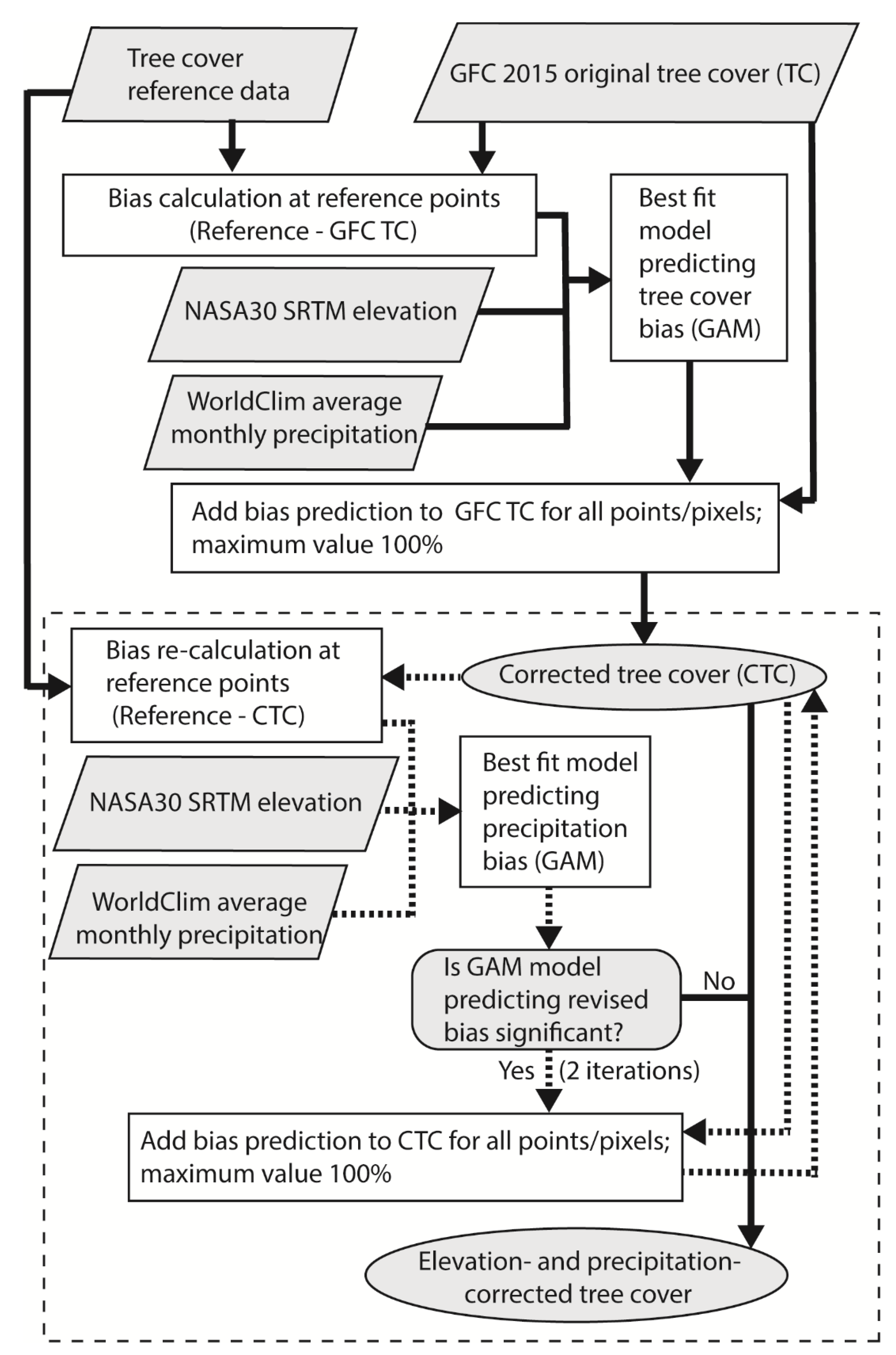
2.1. Reference Tree Cover and Bias Estimation

To assess potential biases in tree cover estimation, we compared GFC tree cover predictions to a reference dataset collected by two trained image interpreters [15]. The reference dataset consisted of randomly selected GFC pixels across Costa Rica (n = 1300); only pixels with valid high-resolution imagery (n = 1154) were assessed (Figure A1). The interpreters used freely available high-resolution data (Google Earth, ArcGIS basemap) to quantify tree cover (0–100%) and identify land use at each 30 × 30 m pixel. In each pixel, a 5 × 6 grid was used to aid estimation of tree cover percentage, and the average tree cover between the two interpreters was used as the reference tree cover estimate. Interpreters used a reference year of 2015; if cloud-free 2015 imagery was not available, the closest available year was used. The majority of samples (87%) were taken within two years of 2015; when samples were collected prior to 2015, Landsat time series were used to confirm that changes in tree cover did not occur through 2015. If changes did occur, ArcGIS basemap imagery was used to update to a more recent year (e.g., 2017). Tree crops within intensively cultivated crop fields were not quantified as tree cover (e.g., oil palm), but hedgerows and shade trees (e.g., trees in coffee fields) were considered tree cover. Any points that resulted in disagreement between interpreters (either in land cover or a >50% difference in tree cover estimates) were re-evaluated to arrive at a consensus reference estimate. Differences in land cover or tree cover > 50% occurred in four instances, and in all cases, they were resolved after discussion (i.e., they arose from individual user error, not disagreements).
At all pixels (n = 1154), GFC-estimated tree cover in the year 2000 was updated to 2015 by setting forest loss pixels to 0% (n = 42) and forest gain pixels to 100% (n = 7). Where both loss and gain occurred in a given pixel (n = 2), cover was set to 100% if the loss occurred prior to 2012. Then, biases in continuous tree cover estimates were quantified by examining pixels that exceeded a high reference tree cover threshold (≥89%) that will hereafter be referred to as “forest cover”. This threshold optimizes forest/nonforest accuracy for the GFC product in Costa Rica (see [15] for percent threshold derivation). Across this subset of “forest” pixels (n = 556), biases in GFC estimates (0–100%) were calculated by subtracting the GFC estimated tree cover from the reference tree cover (forest cover bias = Reference − GFC). Pixels with forest cover biases of ≥ 89% were then omitted (n = 27), as they all represented misclassifications at forest edges, not continuous differences in estimates along gradients. This final pixel subset (n = 529) was used for further bias correction analysis; it contained no pixels corrected for forest loss or gain.

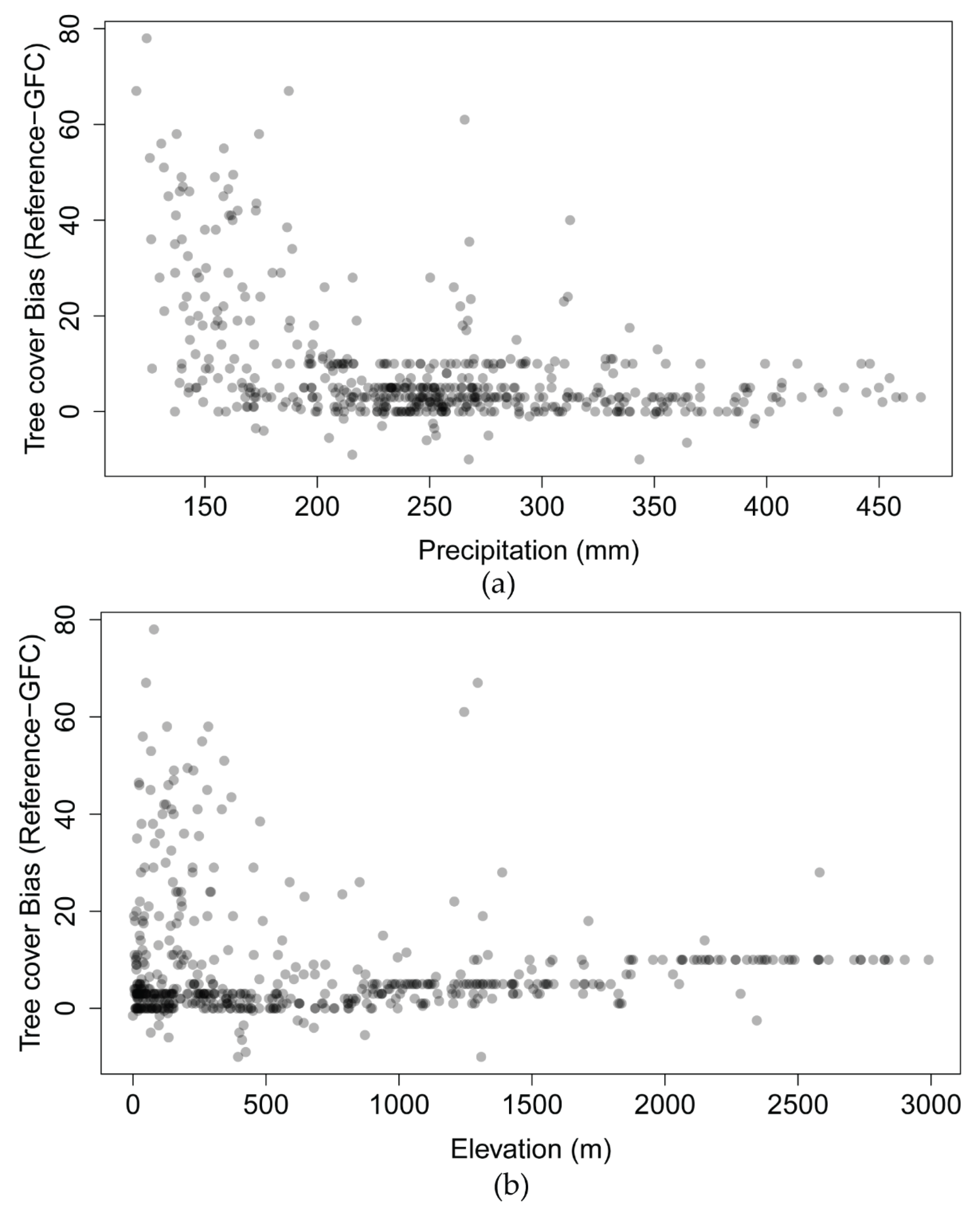
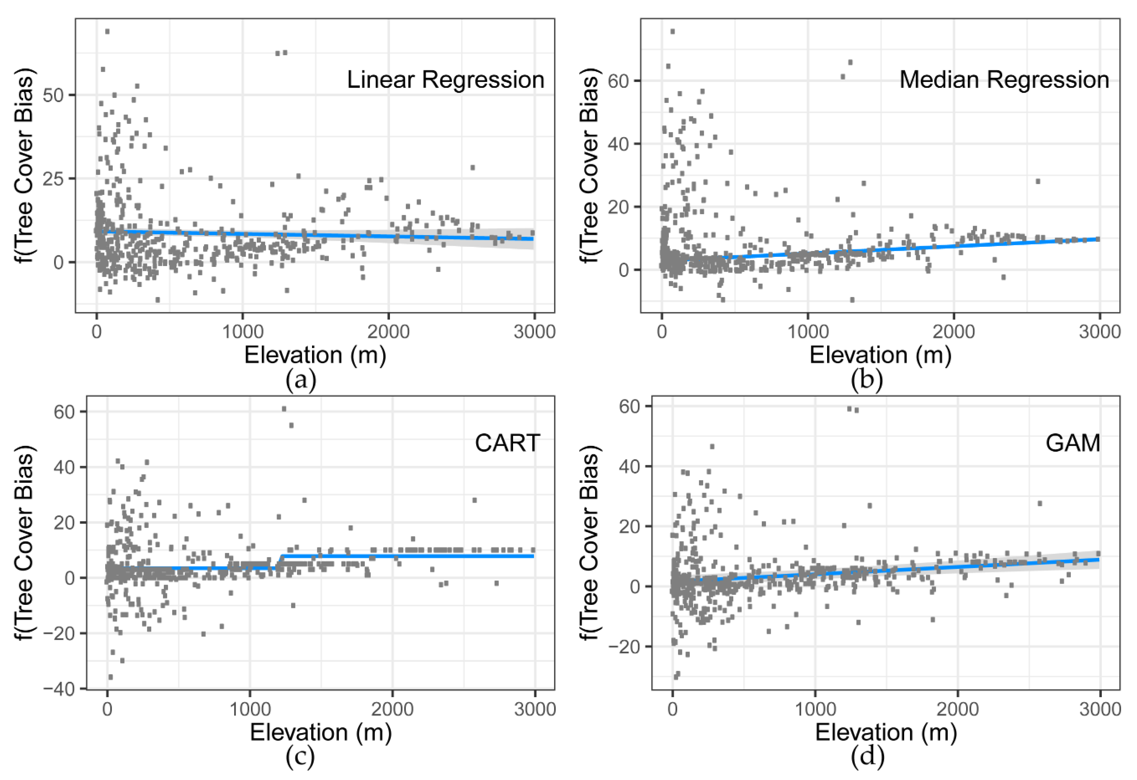
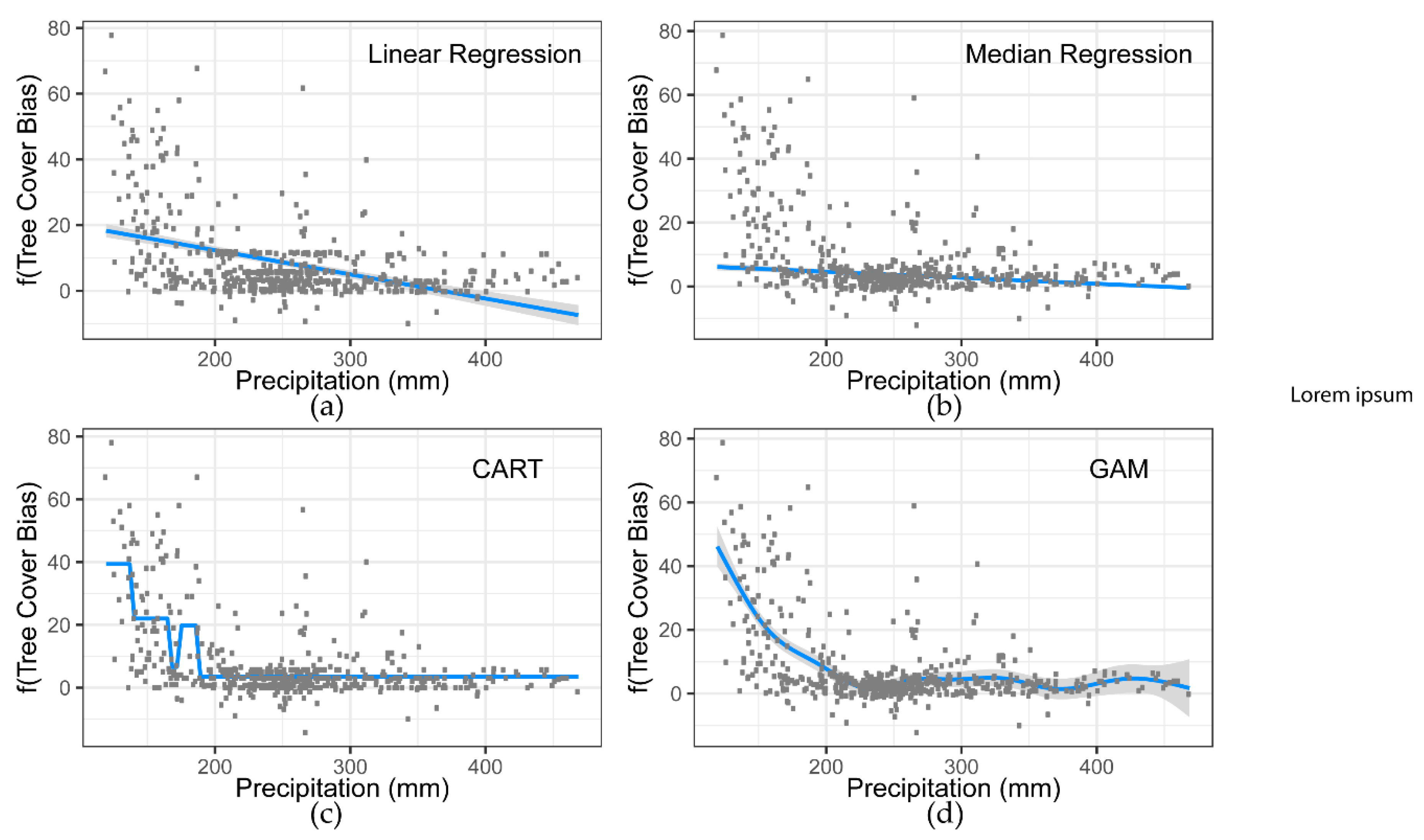
2.2. Modeling Bias along Biophysical Gradients

Biases in tree cover prediction along biophysical gradients were examined, specifically as a function of (a) average monthly precipitation (mm) and (b) elevation (m) (Figure A1 and Figure A2). Precipitation data were resampled from 30 arcsecond WorldClim data (version 1.4; [52]) to 30 m pixels, and elevation data were derived from 30 m SRTM data (version 3.0). Despite observed nonlinearities in biases along both gradients, a previous analysis [15] indicated that significant directional trends in bias existed at high elevation and at low precipitation. Precipitation and elevation were not correlated (r = 0.05; p = 0.30). However, given that regions with low average monthly precipitation were located only at low elevations (Figure A3), it was difficult to distinguish bias arising from elevation from that arising from precipitation. Thus, we chose to examine bias in our statistical models as a function of both elevation and precipitation, but we did not include their interaction term in the models.
To estimate continuous, nonlinear biases across gradients of elevation and precipitation, we tested four different statistical models: linear regression, quantile regression, generalized additive models (GAM), and a classification and regression tree (CART) [53]. The linear regression was a standard OLS regression with a log-transformed response variance, and the quantile regression predicted log-transformed median values; both of these models were selected as basic linear benchmarks. The GAM applied a “ti” smoothing function to the bias data and used a thin plate regression spline with 10 knots. The CART decision tree was implemented in the rpart package in R 3.5.1 with no pruning criteria and default hyperparameters. The performance of each model was evaluated by calculating the root mean-square deviation (RSMD) between model predictions and reference bias values, as well as a visual assessment of model fit.
The resulting best-fit model was used to predict bias as a function of elevation and precipitation. To correct underestimates of tree cover along elevation and precipitation gradients, the model bias prediction was added to all GFC tree cover values, with a maximum possible corrected tree cover value of 100%. Then, using the reference data and this corrected GFC tree cover, bias was re-calculated. To assess whether additional correction was necessary, the same type of best-fit model was fit to the corrected bias values. If any term in the model was significant, indicating that residual bias remained along biophysical gradients, we iterated through the model prediction and bias correction process once again; this methodology is illustrated in Figure 1. This process continued until the best model fit to the corrected values was nonsignificant (p > 0.05). Three successive model fits were required to correct bias in estimates of tree cover; these corrections made the GFC tree cover values more closely resemble values from the validation dataset. In the end, for all pixels, the percent bias estimates from the three model fits were added together, and then added to the GFC tree cover value, with summed tree cover values never allowed to exceed 100%.

2.3. Agricultural Cover Classification

To correct potential biases in GFC tree cover mapping in agricultural systems, we created an agricultural land cover map that classified six major tropical crops: coffee, rice, pineapple, sugarcane, banana, and oil palm. These crops represent six of the seven top species grown in Costa Rica by harvest area (Table A1). To maximize the accuracy of the resulting land cover classification, each crop species was mapped separately and then combined into a six-species agricultural land cover map. However, two of the crops, banana and oil palm, were processed together in one classification model due to sharply increased accuracy; no other combinations improved accuracy (data not shown).
To classify crops, we developed a training dataset that consisted of crop and background points. For each of the six crops, we manually selected 50 data points from a nationwide agriculture dataset. This dataset consisted of field GPS locations collected by the Ministrio de Agricultura y Ganaderia de Costa Rica (MAG) to assess crop pest outbreaks. Then, we added to this data by creating 1050 randomly generated “background” points, omitting and replacing any points within a crop field of one of the six focal species. At each point, we used high-resolution imagery to determine its 2015 land cover and crop type. Then, each of the resulting 1350 points were given a 60-m radius circular buffer polygon. If a buffer polygon overlapped multiple land cover types, it was moved to the nearest location with only a single land cover type. Then, we intersected the buffer polygons with various raster layers (Table 1) to extract training pixel data for each land cover class. The extracted training pixel data were processed and filtered to remove pixels not fully covered by the buffer polygon (<25% of the pixel covered) and entries with recorded forest cover loss.
Then, with the processed pixel data, we used the Random Forest algorithm in R (randomforest package, default hyperparameters; [54]) to individually classify rice, pineapple, sugarcane, banana, coffee, and oil palm in Costa Rica. For each of the five crop species models, all crops not being classified were reclassified as background data. Then, a 1:5 ratio (crop/background) was used to sample the training data (without replacement) to prevent the model from overpredicting crop abundance [55]. Finally, although we attempted to classify coffee individually, our highest coffee class omission accuracy was <60% overall and is not further reported here. Instead, we converted an existing Costa Rica Coffee polygon layer [56] to raster to delimit coffee with Costa Rica, and we report that accuracy below.
For each crop (excluding coffee), we created three different Random Forest classification models. The first set of models (texture) was created using all the raster input data. The second set of models (no-texture) used all the raster input data except for the texture data. We found that models that excluded texture variables (no-texture) were best at predicting agricultural cover within agricultural fields. Since texture was calculated using a moving window, models that included texture tended to map edges of agricultural fields quite poorly and under-predict agricultural cover there. However, models that included texture were better at differentiating agricultural and background cover outside agricultural fields. The third set of models (spectral-only) used only the input spectral data (omitting the ALOS PALSAR and texture data). Visual inspection of maps predicted from ALOS PALSAR data revealed missing data in montane areas, necessitating the spectral-only model to replace missing values. These layers predicted by the models were composited to reflect our observations, as follows.
First, we grouped the crop pixels into distinct patches (queen connectivity) for the no-texture land cover predictions. Second, we eliminated all crop pixel patches from the no-texture land cover map that did not have at least one overlapping crop pixel in the texture land cover map. The resulting revised no-texture crop maps had fewer spurious misclassifications outside agriculture fields, while retaining agricultural field patches. As a final step, we filled in all missing data values with the spectral-only model predictions to replace SAR-related missing data in montane areas.
To increase the accuracy of the classifications, we completed two additional post-processing steps. A sieve filter of 40 pixels (4 ha) was applied to the maps to remove noise from small misclassified areas. Finally, using Guidos Toolbox [57], perforations smaller than 200 pixels within the classified agricultural fields were identified and filled with agricultural cover. Then, we mosaicked the combined, post-processed model output for each crop species. Crops were mosaicked in the following order to create an all-species agricultural classification: sugarcane, rice, pineapple, oil palm, banana, and coffee. The selected mosaicking order was determined visually, based on apparent accuracy, and the resulting map delineated the 2015 agricultural cover of Costa Rica.
The accuracy of the 2015 agricultural cover map was assessed following a stratified random sampling methodology. Independent testing data were randomly generated for each land cover class (stratum). The number of testing points per stratum was determined following the guidelines of Olofsson et al. [58], using stratified accuracy assessment equations (Table A2). At each testing point, we determined the land cover and crop type in 2015 using freely available high-resolution imagery, following the methodology described in Section 2.1. Then, a confusion matrix was used to assess map accuracy, comparing the reference land cover with predicted map cover at each testing point, with the resulting estimates weighted by map area [59].

2.4. Revising GFC Forest Cover

To correct the GFC forest product, we integrated it with our bias corrections for precipitation and elevation, and agricultural land cover map. As a first step, we generated an estimate of 2015 forest cover by combining the GFC tree cover layer (for the year 2000) with the GFC forest loss (2000–2015) and gain layers (2000–2012). By assigning each gain pixel a tree cover value of 100%, we added the gain layers to the original GFC product. Then, we subtracted the GFC loss pixels by assigning them a value of 0% tree cover. If gain and loss pixels overlapped and the loss year was 2012 or greater, then the pixels were assigned 0% tree cover.
Then, we corrected this 2015 forest cover estimate with bias adjustments for precipitation and elevation. First, we used the best-fit model for the elevation and precipitation bias to predict the bias correction for a given DEM elevation and precipitation amount at each pixel, summing the total bias correction across the three best-fit model iterations. Then, we added this bias correction to the tree cover estimate, only increasing tree cover where the original tree cover estimate was ≥30%. Setting a 30% tree cover threshold for increasing tree cover followed international tree cover definitions [14] and limited false-positive increases in tree cover in open habitats, such as pastures and urban areas. After this additive bias correction, the maximum tree cover was capped at 100%, with all higher values recoded to 100%.
Finally, as a last step, biases in agricultural tree cover estimates were corrected using the agricultural cover map. With the exception of coffee, all areas with agricultural cover were given a tree cover value of 0%. Coffee fields contained non-agricultural tree cover, but GFC estimates of tree cover in coffee fields were poorly correlated with actual tree cover, with a distinct distribution of values (linear regression, p = 0.63, Figure A4). Given the large differences in mean and median values between reference tree cover (mean: 40.4%; median: 20%) and GFC estimates (mean 64.1%; median 79.5%), maximum tree cover in coffee fields was set to the mean reference value (40%).
The methodology described above created a revised GFC map product for 2015 that estimated natural tree cover. The accuracies of the original and revised GFC tree cover products were assessed using a second, independent test dataset consisting of randomly located points (n = 732). This second test dataset was created using freely available high-resolution imagery, following the methodology described in Section 2.1.

2.5. Forest Fragmentation Analysis Comparison

To understand how biases in the original GFC product may affect forest analyses using this product, we first used a threshold to convert the original and corrected maps of continuous tree cover into forest/nonforest maps. We used a threshold for the maps that optimized overall map accuracy in a previous study (89%) [15] and set all pixels below the threshold to nonforest. Then, we used the resulting forest/nonforest maps to calculate metrics of forest cover, fragmentation (the area of forest within one pixel of the edge), and connectivity (defined as the area of disconnected forest fragments). We examined forest metrics within (a) protected areas, (b) both protected areas and designated biological corridors [60], and (c) outside protected areas and corridors. Then, we compared the original GFC-derived forest cover and fragmentation metrics with metrics derived from the bias-corrected revised GFC products.
We examined forest cover and fragmentation using the GuidosToolbox Morphological Spatial Pattern Analysis (MSPA) classification [57,61], which processes binary landscape classifications (foreground/background). MSPA classification uses segmentation to categorize the foreground (in this analysis, forest) based on size, shape, connectivity, and spatial arrangement [57,61,62]. The foreground of the binary image is divided up into seven main categories: Core (interior patches excluding the perimeter), Islet (disconnected and too small to have a core), Loop (a linear feature connected to the same core patch), Bridge (a linear feature connected to a different core patch), perforation (internal edge of a core patch), Edge (the perimeter of a core patch), and branch (a linear feature that is connected to an edge, perforation, bridge, or loop [57]). Then, the MSPA classification of forest cover was used to detect and quantity core forest, edge forest, and fragmented forest area (defined below).
Prior to using the thresholded forest/nonforest maps for MSPA classification, we set a minimum mapping unit of two pixels to remove single pixel noise, which had inflated edge and fragmentation results in preliminary analysis. This had the effect of making our assessments of fragmentation less sensitive to small changes in tree cover arising from correction of the GFC tree cover map. For the MSPA analysis, we set the foreground connectivity to eight pixels, the transition setting was turned on, and the intext setting was turned off. Since we simply wished to assess fragmentation and not explore different edge effect distances [63], we used the default edge width setting of one pixel (30 × 30 m).
The output of each foreground classification had 12 different classes, given the occurrence of pixels in intersecting classes [61]. For each of the areas of analysis (protected areas, protected areas and corridors together, and background areas), we calculated the total core forest area, total forest edge area, and total forest fragment area. Using this data, we also calculated the total core area index (CAI) [64], which is the area of core forest divided by the total forest area. The total core forest area was calculated using the “core” MSPA class, and fragmented forest was calculated using the “islet” MSPA class (i.e., edge forests not connected to the core forest area). Edge forest was calculated by combining all other classes, and it consisted of edge forest pixels that were connected to the core forest area (i.e., along the margin of core forest).
Then, we summed each area metric across the three protection classes (protected area, protected area and corridor, or background area) and standardized by dividing by the total area in each class. Similarly, mean CAI across all features was calculated for each protection class. These calculations were done for the GFC product and each of the revised GFC products (precipitation and bias corrected cover, agriculture corrected cover, and the combined, final revised GFC cover). Additionally, for each feature (e.g., an individual protected area), the percent change in area metrics was calculated by subtracting the original GFC pixel totals from the revised GFC product pixel totals and then dividing the difference by the total number of pixels in that feature.

3. Results

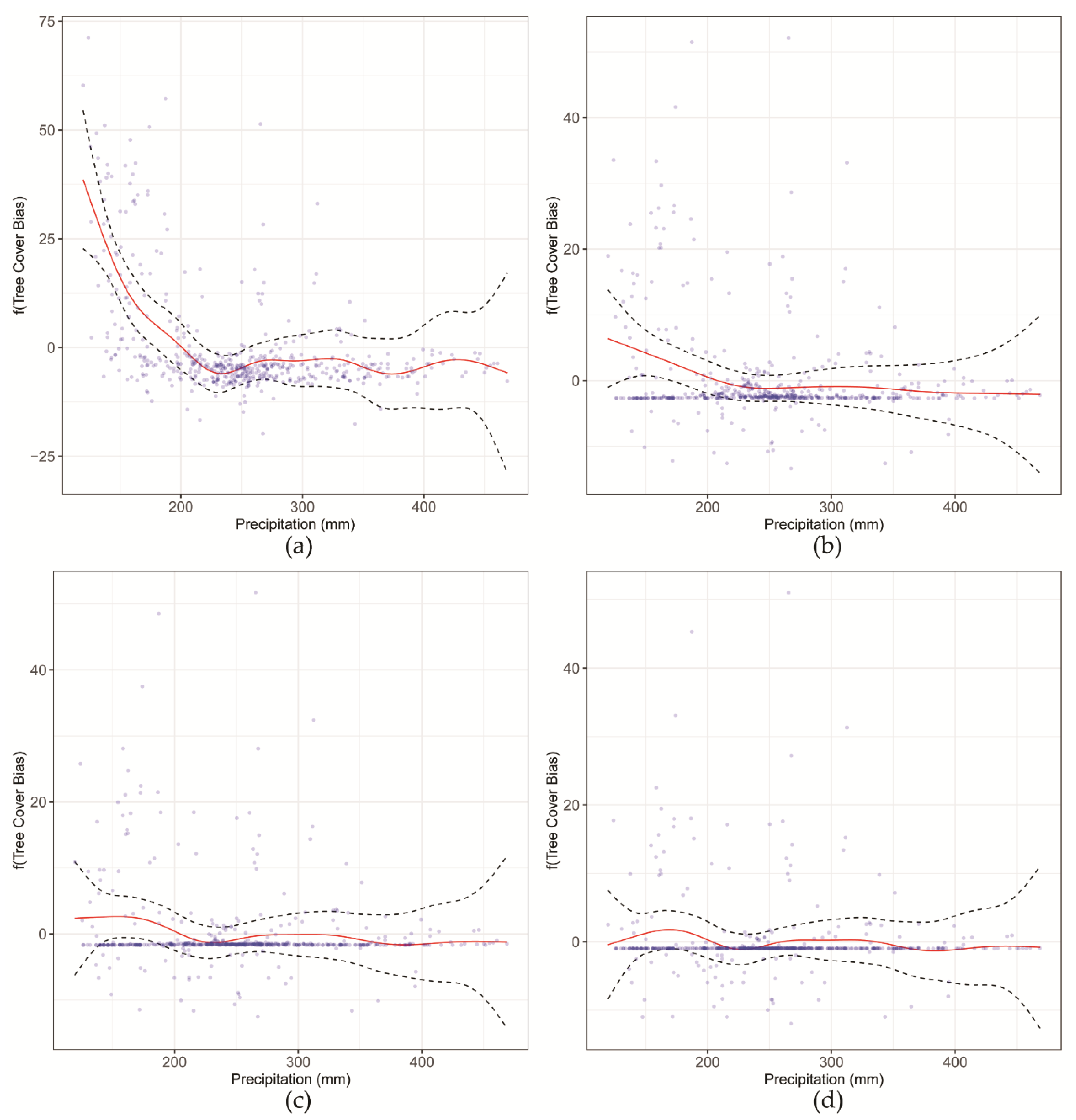
3.1. Elevation and Precipitation Bias Assessment and Correction

Prior to correction, GFC tree cover estimate bias (i.e., the difference between GFC-predicted and reference tree cover values) ranged from −10% to 78%. A previous study [15] found that at elevations above 370.5 m, GFC bias significantly increased to a maximum of 10% (Figure 2). Much higher levels of observed GFC bias were observed at low elevations, where they significantly increased as precipitation declined, rising to a maximum of 78% (<189 mm; Figure 3 and Figure A3) [15]. Of the four statistical models fit to correct the elevation bias, the CART model had the lowest RSMD (Table 2), and its flat prediction trajectory at higher, unsampled elevations (>3000 m) matched the flat trend in the bias above 2000 m. However, no model was able to exactly reproduce the stepwise trend in bias values with increasing elevation (Figure 2 and Figure 3), and two of the statistical models had low RSMD—the CART and the GAM models (Table 2). Furthermore, the trend in the sample at low levels of precipitation was clearly upwards, as is reflected in the GAM prediction trend, while the decision tree prediction trend was flat with decreasing precipitation (Figure 4). To better fit out-of-sample observations at lower levels of precipitation, the GAM model was selected as the final model (Figure 3d, Figure 4d and Figure A5a; general additive model, p < 0.0001).
However, after correcting the tree cover data with the GAM model (see Section 2.2 and Figure 1 for methodology), a second GAM fit to the corrected residuals indicated that bias with respect to precipitation remained in the dataset (GAM; p < 0.0001; Figure A5b). Thus, the dataset was corrected a second time by using this second GAM model. However, after a second correction, a third GAM of the corrected residuals indicated that bias with respect to precipitation persisted (GAM; p < 0.0016; Figure A5c). This third GAM prediction was applied to correct the residual dataset. Finally, a fourth GAM on the corrected residuals indicated that no bias with respect to precipitation remained (GAM, p = 0.086, Figure A5d). This iterative correction method created a final residual dataset with no significant trend with respect to precipitation or elevation.
The three iterations of GAM model corrections for estimate bias increased tree cover linearly with elevation, by 0–10% (Figure 3d). Visual inspection indicated that there was no apparent ecological pattern to the corrected elevation errors, except that they were more common at higher elevations. By contrast, the GAM model corrections for precipitation bias (Figure A5) increased tree cover estimates nonlinearly along a gradient of precipitation, by as much as 70% in low precipitation areas (<189 mm). Visual inspection indicated that tropical dry forests saw the largest tree cover increases (Figure A6, Figure A7, Figure A8 and Figure A9).

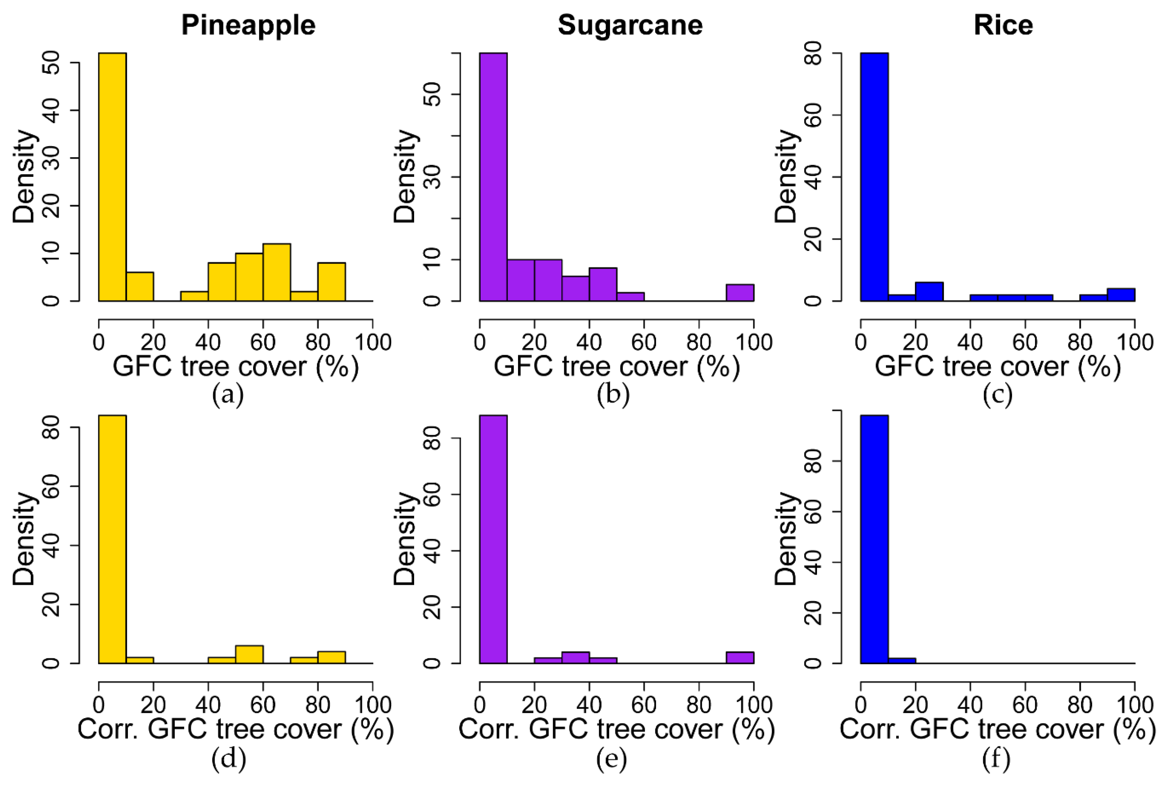
3.2. Agricultural Cover Bias Assessment and Correction

The accuracy assessment performed on the 2015 agriculture land cover map (Table 3 and Table A3) had an overall accuracy of 97.0% and a kappa value of 0.78. The producer’s accuracies ranged from 37% to 100%, while the user’s accuracies ranged from 67% to 99%. Sugarcane (37%) and oil palm (66%) had the lowest producer’s accuracy (low accuracy of omission) of all the crop species. Although only a few reference data points were omitted in each class (Table A3), the large area of non-agricultural background biased the omission errors downward, leading to a large shift in estimated omission error after area correction [65]. The sugarcane classification was conservative in under-predicting sugarcane extent, omitting small sugarcane fields. By contrast, the oil palm classification omitted the very edges of fields, but it mainly did not classify young oil palm fields (<3 years in age) well; this particular error likely had a minimal effect on correction of the 2015 tree cover map, which did not track forest gain <3 years in age (i.e., after 2012).
Although user’s accuracies were higher, rice (67%) and sugarcane (72%) had the lowest user’s accuracies. Visual inspection and Food and Agriculture Organization (FAO) crop statistics (Table A1) indicated that rice was the most overpredicted, followed by sugarcane. However, the overprediction of these two crops did not appear to affect the revised forest cover estimates because overprediction mainly occurred in wet pastures and swamps with <30% tree cover.
After the agricultural cover mask was applied to the GFC cover product, the number of agricultural training points with tree cover > 0% was reduced from 64% to 23% (Table 4), with the sharpest drops for banana, oil palm, and sugarcane. The GFC product had widespread bias in tree cover estimates in agricultural land cover (Figure 5 and Figure 6). Tree cover in perennial erect crops (banana, oil palm, and coffee) was particularly overpredicted. Of the 300 agricultural training points examined, 54% of the points had GFC tree cover > 30% (Figure 5 and Figure 6), across all crop species.

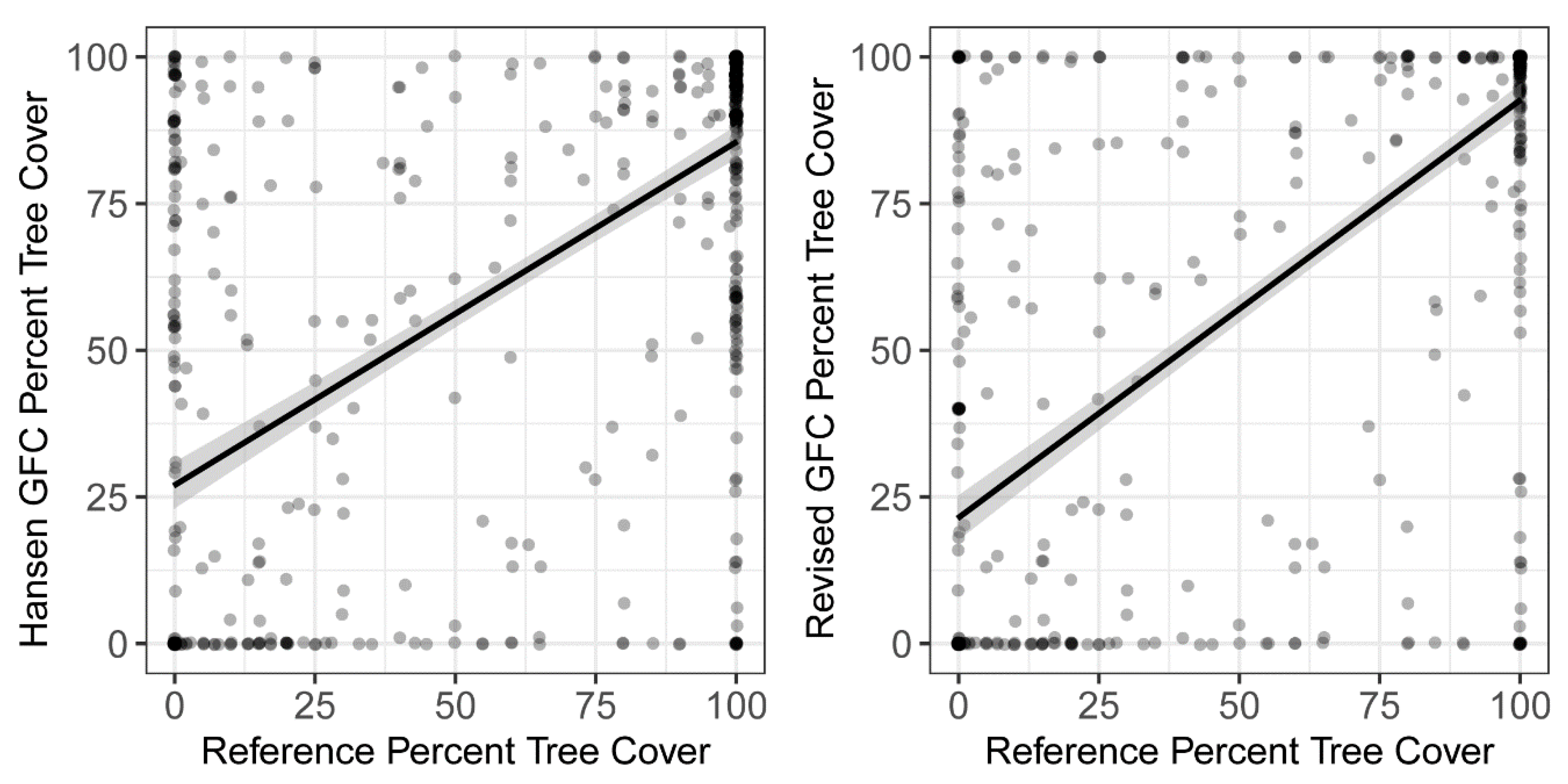
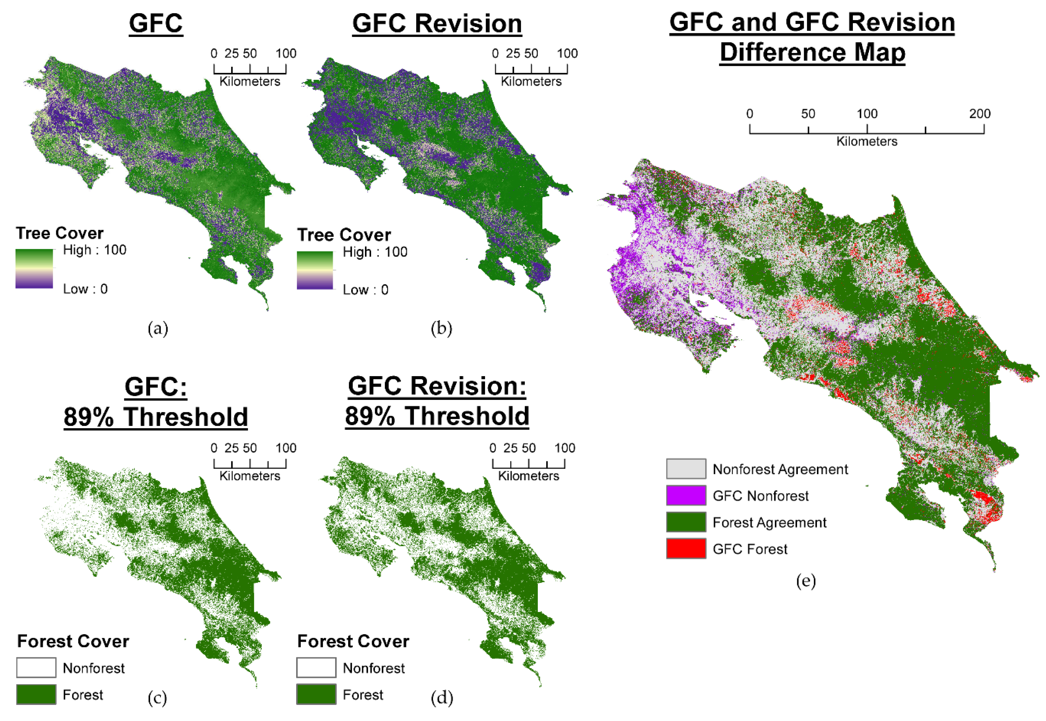
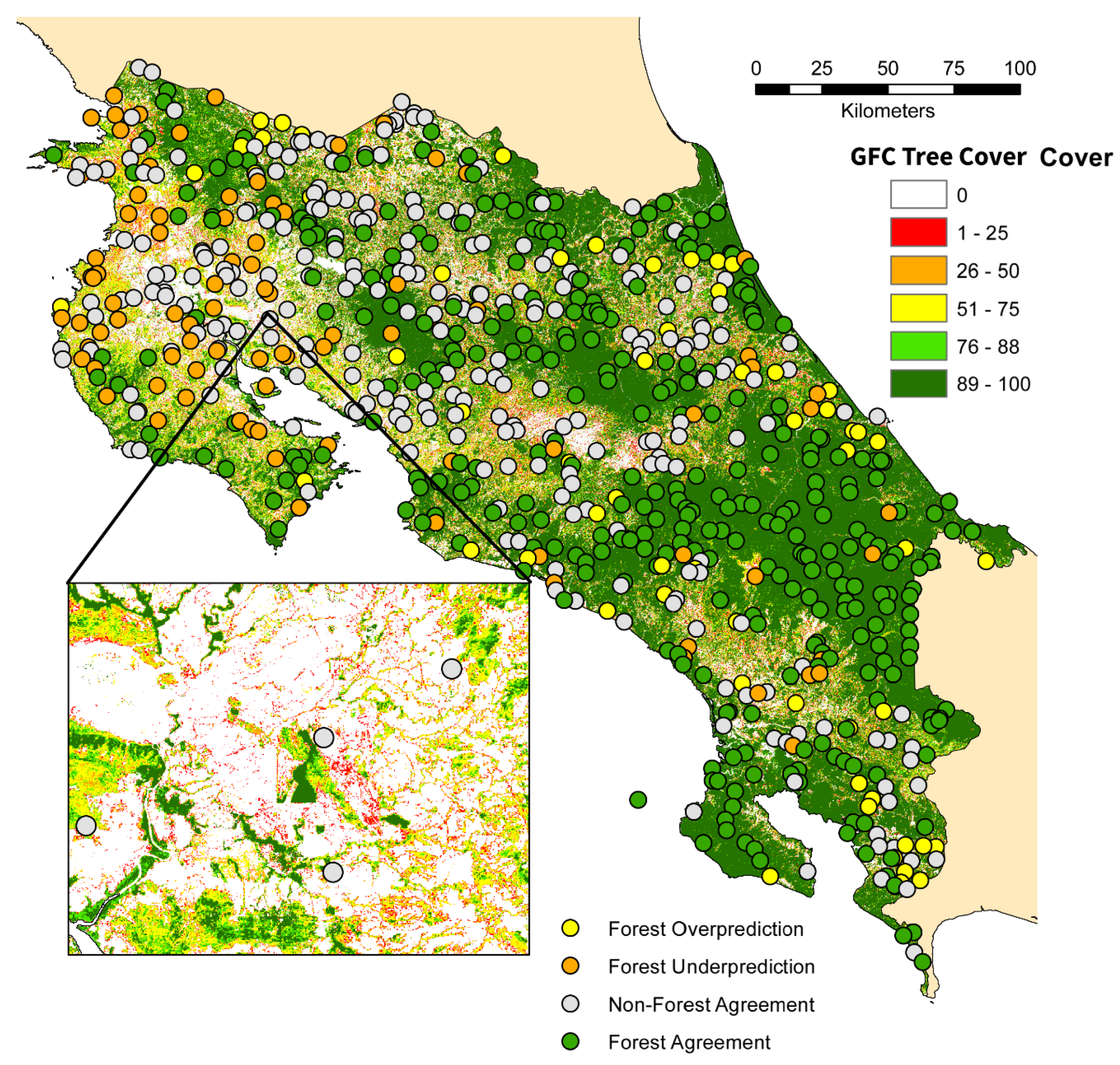
3.3. Corrected Forest Cover Comparison

The original GFC 2015 tree cover product predicted some of the variation in the reference percent tree cover (p < 0.0001, R2 = 0.416), but the revised GFC tree cover product had ≈1.3x better overall accuracy (p < 0.0001, R2 = 0.538; Figure 7). Comparison of the original and revised GFC 2015 maps showed that the bias corrections, taken together, increased the mean percent tree cover from 64.3% to 67.0% (Figure 8a,b and Figure A6, Figure A7, Figure A8 and Figure A9). Total forest cover (tree cover ≥ 89%) increased from 51.3% to 57.4%, with most of the increase occurring in the northwest region of Costa Rica (Figure 8c–e), where tropical dry forest is common. Correcting for elevation and precipitation biases increased forest cover by 8%, while correcting for agricultural errors decreased forest cover by 2%, largely in the central coffee-growing regions and the Atlantic and Pacific coastal plains.
The original GFC forest/nonforest map had an overall accuracy of 79.7%, while the revised GFC forest/nonforest map had an overall accuracy of 85.0% (Table 5 and Table A4). Correcting only the precipitation and elevation errors increased the overall accuracy (83%) and forest class accuracy, but it did not improve the nonforest omission error (i.e., agricultural fields were classified as forest; Table A4). Correcting only the agricultural errors also raised the overall accuracy (81.7%), but it only improved the nonforest omission error and forest commission error (decreasing misclassification of agriculture as forest). The final revised GFC forest/nonforest map had balanced, high accuracy for each class (Table 5 and Table A4), and corrected area estimates closely matched map area estimates [59]. The original GFC forest map had a clear spatial pattern in omission and commission errors, with the omission error for the forest class higher in the northwest tropical dry forest (Figure 9), but the revised forest map had no apparent pattern in errors (Figure 10).
When comparing the GFC and revised product’s forest cover estimates for 2015, the core forest area largely mirrored the total forest area, with larger increases in biological corridors and protected areas than background areas (Figure 11). At an edge depth of one pixel (30 m), core forest increased from 66.7% to 77.1% in protected areas, but it only increased from 25.1% to 28.1% in unprotected background areas. The largest increase in core forest occurred on the Nicoya peninsula where the landscape is dominated by dry tropical forests (Figure 12). In the case of Palo Verde National Park, correcting forest cover estimates increased the core forest area by 725% (Figure 13). By contrast, the core forest cover decreased in areas dominated by agriculture, with the largest decreases occurring in the coastal humid lowlands, where oil palm and banana are grown. Core forest also decreased somewhat in highland regions where coffee production is dominant (Figure 12).
The edge forest area declined in protected areas, but it increased slightly when including biological corridors and in background areas (≈2% of the area of Costa Rica; Figure 11). The largest increases in edge forest area occurred in northwestern dry forests, as the total forest area increased (Figure 12). The edge forest area also increased in several biological corridors adjacent to agricultural regions, and it declined somewhat in the eastern half of the country. On balance, increases in both core area and edge area led to less fragmentation overall (core area index increased; Figure 11). However, the core area index declined in agricultural regions, where “core forest” was removed by the correction (Figure 11). For example, this correction altered estimated fragmentation and connectivity outside Manual Antonio National Park, in the Aguirre Biological Corridor (Figure 13). Due to the relatively shallow edge depth selected, isolated edge-dominated forest fragments (islets) were rare overall, and in general, they decreased by a fraction of a percent across protected areas, corridors, and background areas (Figure 11). The forest fragment area decreased uniformly across most of Costa Rica, except for on the western coast (Figure 12).

4. Discussion

Dry forest cover has been particularly underestimated in global tree cover maps based on optical satellite data [19]. Our correction approach is promising for semiarid tropical regions, as we were able to revise the dry tropical forest cover estimates by as much as 70% while leaving wet tropical forest estimates unaffected. The presence of biases in the GFC and other forest products along a precipitation gradient has been previously documented [15,19,40]. This underestimate is possibly due to the difficulties of distinguishing sparse forests against their understory background, and/or in detecting closed canopy forests in the dry season with low leaf cover [40]. Other remote sensing solutions have been applied at local to regional scales to map dry/deciduous forest cover, including resolving tree canopies in high-resolution imagery [19,66], using cloud-composited wet season optical imagery [67,68], quantifying and classifying inter- and intra-annual variation in phenology [69,70,71], and using SAR data to map wet-season tree cover [72]. However, currently, there are no accurate predictions of dry forest tree cover at a global scale. The methodology demonstrated here could potentially permit global maps of dry forest cover, building on existing global forest maps and imagery composites. Additional research is needed to understand whether statistical precipitation corrections are viable in other tropical countries with distinct precipitation gradients and dry forest spatial distributions.
Elevation biases in land cover estimates have also been well researched [73], although efforts have been largely focused on correcting optical imagery for topographic effects on reflectance (e.g., shadowing) using a variety of methods [74,75,76]. The generalized additive model approach tested here is distinct from previous topographical correction methods, but the source of the bias was unclear, and given that it increased in a discrete manner with elevation, it was unlikely to be caused by shadowed topography. The GAM correction was selected based on the structure of the bias and corrected distinct steps in the dataset that may have arisen from the decision tree classification used to create the GFC tree cover map [28,77,78]. We have observed similar errors in the GFC with elevation in other geophysical regions, including the Andes and Himalayas (unpublished data). Although elevational bias errors were relatively small (≤10%) in this study, they may be affecting hydrological [43], landslide [79], and carbon models [12] built using the GFC data.
Even though it only covered six economically important crops, the agricultural land cover map was able to accurately mask many agricultural fields misclassified as forest in the GFC product. This re-classification of agricultural cover was necessary to manually correct the GFC product’s tendency to consistently classify agricultural crops as forest cover [15,21]. For one agricultural species (oil palm), the GFC’s general definition of forest as tree cover >5 m in height [21] caused observed errors. However, many of the corrected errors arose in fields of row crops or in erect crops <5 m in height (pineapple, rice, sugarcane, and banana). Furthermore, there was no observed correlation between coffee cover and estimated GFC tree cover, although GFC tree cover estimates were generally biased upwards in coffee fields. This indicates that shade tree cover in coffee agricultural systems was not accurately mapped by the GFC, and our correction of tree cover in these agricultural systems was only approximate.
Although distinguishing agricultural cover is challenging at regional to global scales [80], it is critical for tracking agricultural expansion and correcting agricultural misclassification. Accurate regional maps have been made for crops such as sugarcane [81], oil palm [82], rubber [83], eucalyptus [84], and banana [85]. Furthermore, it may be possible to use a Landsat-SAR fusion approach similar to the one in this study to assist the mapping of global crop types [86,87] and improve the utility of the GFC product in agricultural regions. However, certain agricultural systems remain quite challenging to distinguish with remote sensing: for example, in this study, we failed to accurately map coffee cover. This is consistent with other efforts to map agroforestry systems such as coffee [88], which are often confused with natural forest cover due to the presence of perennial shrubs and shade trees [89].
The final revised GFC forest cover estimate in this study used a combination of precipitation, elevation, and agricultural bias corrections. Overall, the corrected forest cover product increased the R2 of the predicted tree cover by ≈1.3x and increased the overall map accuracy of the thresholded forest/nonforest product by ≈5%. The correction of the precipitation and elevation biases had a larger impact on map accuracy than the agricultural cover corrections. The agricultural corrections decreased tree cover, while the precipitation and elevation corrections increased it. Other biophysical gradients could also have been important for correcting and improving the GFC tree cover map, including intrannual variability in precipitation, slope, or soil type. Further study is needed to understand global bias patterns in predicting tree cover across many different biophysical gradients. Although the GFC is one of the most widely used tree cover maps, the biases examined here extend to other tree cover products as well [40].
The corrections undertaken in this study led to marked changes in tree cover and fragmentation estimates across Costa Rica. When the GFC and revised products were compared, estimated tree cover, core forest area, and edge forest area increased, and isolated forest fragment area and core area fragmentation decreased. Dry tropical forests within corridors and protected areas experienced the largest estimated increases of overall tree cover and core forest; Palo Verde National Park had more than seven times as much core forest after correction (Figure 13). Agricultural areas saw the sharpest decline in estimated forest cover. The increase in estimated edge forest is likely in part due to the removal of agricultural fields and patches, which created new forest edges. In addition to the increase in core forest, the area of forest islets (thin, disconnected fragments) decreased when comparing the revised product to the GFC. Since patch isolation can be used as a proxy for connectivity [90], the forest connectivity in Costa Rica is generally higher than what could have been previously estimated with the GFC product. However, agricultural corrections led to local declines in connectivity in key regions; for example, after removing oil palm fields from forest cover estimates, the Aguirre Biological Corridor had lower connectivity between montane forests and the lowland Manuel Antonio National Park (Figure 13; [91]). These results indicate that estimates of forest cover, fragmentation, and connectivity using the global GFC product should proceed with caution, particularly in tropical dry forest areas and where tropical agricultural cover is high. The GFC has been widely used for assessing forest function and conservation [34,92], often uncritically.
It is likely that the methodology used here could be successfully adapted to correct the GFC product in other tropical countries and perhaps globally. Despite the cost in time and effort taken in this study to produce a reference data set of tree cover and map agricultural cover, there are three approaches that could lower the burden of this investment. First, many countries already possess detailed information on agriculture and other land cover types (e.g., pastures, mangroves, and swamps) that can be used for improving global forest cover maps (e.g., [93]). Existing geospatial data could directly correct the GFC product—for example, consider the coffee vector data incorporated into our agricultural cover map. Even where land cover data is unavailable, the reference data required to correct the GFC map in this study (n = 1154) is a fraction of the data recently required to map the entire country (n = 31,395, [68]). Second, global data on fractional canopy cover is available from the IceSAT-1, IceSAT-2, and GEDI spaceborne lidar missions [94]. These large, pantropical samples of tree cover could be used to detect and correct biases in wall-to-wall tree cover estimates across national borders and biomes. Our methods depended on an accurate reference dataset, and a broader sample derived from global lidar data might have improved the correction. Third and finally, correcting high-quality global maps can result in higher accuracy than local country-level maps [15], and they can be corrected at a much lower cost. For example, Sannier et al. [26,95] used semi-automated classification and regression models to estimate forest cover using the GFC in regions of Gabon.
Although this study has focused on the GFC, it is one global map among many, and it was used as an example of how we can detect and correct biases in land cover products, revising existing data to better support current conservation efforts while improved maps are under development. Recent advances in both global and regional forest cover maps have been rapid, driven by interest in REDD+, freely available data from NASA and ESA, and free computing resources such as Google Earth Engine [96]. However, despite a burgeoning number of published global maps, efforts to map tropical forests should consider leveraging prior work to maximize efficiency and accuracy. For example, McRoberts et al. [97] improved forest cover in Santa Catarina, Brazil, by using estimators to combine local and global forest cover maps together. Both McRoberts et al. [97] and this study demonstrate complementary strategies on how to revise tree cover estimates in tropical counties by integrating local and global information.

5. Conclusions

Tree cover biases are present in the most widely used global forest cover product, but in this demonstration study, the biases were predictable and correctable across a diverse set of tropical ecosystems. By correcting the tree cover biases, we were able to determine that GFC underestimated forest cover and overestimated fragmentation for 2015 in Costa Rica, especially in tropical dry forests. Potential future avenues of research include evaluating the impact of correcting the GFC data on estimates of connectivity and carbon storage. Although the GFC correction methodology was not evaluated outside Costa Rica, we believe that this methodology is transferable to other tropical countries with similar gradients in precipitation, elevation, and agricultural cover.

Author Contributions

These authors contributed to the following: conceptualization, methodology, software, formal analysis, investigation, writing—original draft preparation, writing—review and editing, and visualization, D.C.; M.E.F.; validation and data curation, D.C.; P.C.; supervision, resources, project administration, and funding acquisition, M.E.F. All authors have read and agreed to the published version of the manuscript.

Funding

This research received no external funding.

Acknowledgments

We would like to thank Matthew Baker for technical and statistical guidance. We would also like to thank Maggie Holland for her feedback on earlier drafts of this manuscript.

Conflicts of Interest

The authors declare no conflict of interest.

Appendix A

Figure A1. Elevation across Costa Rica with locations of the bias correction reference data shown. Note the central mountain range running northwest–southeast.
Remotesensing 12 03226 g0a1
Figure A2. Precipitation across Costa Rica with locations of bias correction reference data shown. Note differences in rainfall between the east and west of the country.
Remotesensing 12 03226 g0a2
Figure A3. Scatterplot of precipitation and elevation values at reference data locations across Costa Rica. Darker colors indicate higher densities of points, and the blue vertical line indicates precipitation of 2000 mm annually (≈167 mm on average per month), which is the Holdridge threshold for the low-elevation dry forest biome.
Remotesensing 12 03226 g0a3
Figure A4. Plot of reference coffee tree cover (agricultural training data, n = 50) against GFC estimated tree cover in 2015. The histograms of each variable are shown on the x and y axes, with median and mean values labeled.
Remotesensing 12 03226 g0a4
Figure A5. The fit of the three iterations of GAM models to the calculated bias in tree cover estimates is shown, with the partial term for precipitation displayed. Panel (a) shows the fit from the first iteration, panel (b) shows the fit from the second iteration, and panel (c) shows the fit from the third iteration (Figure 1). Panel (d) shows a fourth iteration of precipitation against the bias remaining in the final revised GFC tree cover data; this fourth GAM is nonsignificant (p = 0.48).
Remotesensing 12 03226 g0a5
Figure A6. Original GFC estimated tree cover across Costa Rica (2015) displayed to emphasize bias patterns. Note differences in estimated tree cover between the east and west of the country; similar trends do not exist in the reference tree cover data.
Remotesensing 12 03226 g0a6
Figure A7. Partly corrected GFC estimated tree cover across Costa Rica (2015) displayed to emphasize bias patterns. This map has been corrected for precipitation and elevation errors but not agriculture. Note the lack of differences in estimated tree cover between the east and west of the country.
Remotesensing 12 03226 g0a7
Figure A8. Partly corrected GFC estimated tree cover across Costa Rica (2015) displayed to emphasize bias patterns. This map has been corrected for agricultural errors but not precipitation and elevation. Note the absence of tree cover in the coastal and central agricultural regions as well as remaining differences in estimated tree cover between the east and west of the country.
Remotesensing 12 03226 g0a8
Figure A9. Fully revised GFC estimated tree cover across Costa Rica (2015) displayed to emphasize bias patterns. This map has been corrected for precipitation, elevation, and agricultural errors.
Remotesensing 12 03226 g0a9
Table A1. FAO statistics of agricultural harvest in Costa Rica by area.
Top Costa Rican Crops by Area Harvested, 2015
CropArea Harvested (km2)FAOstat Description
Coffee, green841.33Official data
Oil palm fruit694.26Official data
Sugarcane646.76Official data
Fruit, fresh *510.62FAO data based on imputation
methodology
Rice, paddy489.01Official data
Banana430.24Official data
Pineapple400.00Official data
* “Fruit, fresh” was not included in the land cover classification because it is not one species or land cover type.
Table A2. For a stratified random assessment of the agricultural land cover map, the number of testing points per stratum was determined following the guidelines of Olofsson et al. (2014). The allocation of points in each stratum was determined through iterative conjecture [58].
Strata(i)Mapped Proportion (Wi)Conjectured Values of Accuracy (Ui)Standard Deviation of Strata (Si)Final Allocation
Background0.9220.850.357675
Rice0.0270.850.357100
Sugarcane0.0030.850.357100
Pineapple0.0090.850.357100
Banana0.0100.850.357100
Palm0.0090.850.357100
Coffee0.0190.850.357100
Total Units (n) 1275
Table A3. Accuracy assessment for the 2015 agricultural land cover map, showing the original reference data. Agricultural testing points (n = 1274) were located through a stratified random sampling design. See Table 3 for the area-corrected accuracy estimate.
Agricultural Land Cover Map Accuracy
Reference
ClassifiedBgRiScPaBaOpCoTotalUsers
Background (Bg)66403 13367499%
Rice (Ri)3267 1 10067%
Sugarcane (Sc)28 72 10072%
Pineapple (Pa)81191 10091%
Banana (Ba)7 1 92 10092%
Oil palm (Op)11 188 10088%
Coffee (Co)19 8110081%
Total7696877919492841274
Producers86%99%94%100%98%96%96%
Overall Accuracy 89.2%
Table A4. Area-corrected user’s, producer’s, and overall accuracy of different forest/non-forest maps at the 89% forest cover threshold. Overall accuracy and corrected area estimates are shown (mean ± 95% confidence interval), with original confusion matrix point counts in italic parentheses.
Reference Data Thresholded at 89%
GFC, Original (2015)Reference Data
PredictedNonforestForestTotalUser Acc.Original Map Area (km2)
Nonforest0.3623 (259)0.1245 (89)0.48774.429,571
Forest0.0788 (59)0.4343 (325)0.51384.631,167
Total0.44120.55881OverallCorrected Area (km2)
Prod. Acc.82.177.7 79.7
±2.9
NF: 26,797 ± 1763
For: 33,941 ± 1763
Precip/Elev Corr.Reference Data
PredictedNonforestForestTotalUser Acc.Original Map Area (km2)
Nonforest0.3365 (244)0.0703 (51)0.40782.724,709
Forest0.1004 (74)0.4927 (363)0.59383.136,030
Total0.43690.56311OverallCorrected Area (km2)
Prod. Acc.77.087.5 82.9
±2.7
NF: 26,538 ± 1658
For: 34,200 ± 1658
Ag Corr. OnlyReference Data
PredictedNonforestForestTotalUser Acc.Original Map Area (km2)
Nonforest0.3823 (274)0.1242 (89)0.50675.530,763
Forest0.0588 (44)0.4347 (325)0.49488.129,975
Total0.44120.55881OverallCorrected Area (km2)
Prod. Acc.86.777.8 81.7
±2.8
NF: 26,795 ± 1686
For: 33,943 ± 1686
Revised GFCReference Data
PredictedNonforestForestTotalUser Acc.Original Map Area (km2)
Nonforest0.3563 (259)0.0702 (51)0.42683.525,901
Forest0.0802 (59)0.4934 (363)0.57486.034,838
Total0.43650.56351OverallCorrected Area (km2)
Prod. Acc.81.687.6 85.0
±2.6
NF: 26,510 ± 1574
For: 34,228 ± 1574

References

  1. Lewis, S.L.; Edwards, D.P.; Galbraith, D. Increasing human dominanceof tropical forests. Science (80-) 2015, 349, 827–832. [Google Scholar] [CrossRef] [PubMed]
  2. Gibson, L.; Ming Lee, T.; Koh, L.P.; Brook, B.W.; Gardner, T.A.; Barlow, J.; Peres, C.A.; Bradshaw, C.J.A.; Laurance, W.F.; Lovejoy, T.E.; et al. Primary forests are irreplaceable for sustainingtropical biodiversity. Nature 2011, 478, 378–381. [Google Scholar] [CrossRef] [PubMed]
  3. Venter, O.; Laurance, W.F.; Iwamura, T.; Wilson, K.A.; Fuller, R.A.; Possingham, H.P. Harnessing Carbon Payments to Protect Biodiversity. Science 2009, 326, 1368. [Google Scholar] [CrossRef] [PubMed]
  4. Kindermann, G.; Obersteiner, M.; Sohngen, B.; Sathaye, J.; Andrasko, K.; Rametsteiner, E.; Schlamadinger, B.; Wunder, S.; Beach, R. Global cost estimates of reducing carbon emissions through avoided deforestation. Proc. Natl. Acad. Sci. USA 2008, 105, 10302–10307. [Google Scholar] [CrossRef] [PubMed] [Green Version]
  5. Vijay, V.; Pimm, S.L.; Jenkins, C.N.; Smith, S.J. The Impacts of Oil Palm on Recent Deforestation and Biodiversity Loss. PLoS ONE 2016, 11, e0159668. [Google Scholar] [CrossRef]
  6. Gibbs, H.K.; Ruesch, A.S.; Achard, F.; Clayton, M.K.; Holmgren, P.; Ramankutty, N.; Foley, J.A. Tropical forests were the primary sources of new agricultural land in the 1980s and 1990s. Proc. Natl. Acad. Sci. USA 2010, 107, 16732–16737. [Google Scholar] [CrossRef] [PubMed] [Green Version]
  7. Grainger, A. Uncertainty in the construction of global knowledge of tropical forests. Prog. Phys. Geogr. 2010, 34, 811–844. [Google Scholar] [CrossRef] [Green Version]
  8. Kaiser, J. Satellites Spy More Forest Than Expected. Science 2002, 297, 9–10. [Google Scholar] [CrossRef]
  9. Kleinn, C.; Corrales, L.; Morales, D. Forest area in costa rica: A comparative study of tropical forest cover estimates over time. Environ. Monit. Assess. 2002, 73, 17–40. [Google Scholar] [CrossRef]
  10. Grainger, A. Difficulties in tracking the long-term global trend in tropical forest area. Proc. Natl. Acad. Sci. USA 2008, 105, 818–823. [Google Scholar] [CrossRef] [PubMed] [Green Version]
  11. Grinand, C.; Rakotomalala, F.; Gond, V.; Vaudry, R.; Bernoux, M.; Vieilledent, G. Estimating deforestation in tropical humid and dry forests in Madagascar from 2000 to 2010 using multi-date Landsat satellite images and the random forests classifier. Remote Sens. Environ. 2013, 139, 68–80. [Google Scholar] [CrossRef]
  12. Achard, F.; Beuchle, R.; Mayaux, P.; Stibig, H.; Bodart, C.; Brink, A.; Carboni, S.; Desclee, B.; Donnay, F.; Eva, H.D.; et al. Determination of tropical deforestation rates and related carbon losses from 1990 to 2010. Glob. Chang. Biol. 2014, 20, 2540–2554. [Google Scholar] [CrossRef] [PubMed]
  13. Chazdon, R.L.; Brancalion, P.H.S.; Laestadius, L.; Bennett-Curry, A.; Buckingham, K.; Kumar, C.; Moll-Rocek, J.; Vieira, I.C.G.; Wilson, S.J. When is a forest a forest? Forest concepts and definitions in the era of forest and landscape restoration. Ambio 2016, 45, 538–550. [Google Scholar] [CrossRef] [PubMed]
  14. Sexton, J.O.; Noojipady, P.; Song, X.-P.P.; Feng, M.; Song, D.-X.X.; Kim, D.-H.H.; Anand, A.; Huang, C.; Channan, S.; Pimm, S.L.L.; et al. Conservation policy and the measurement of forests. Nat. Clim. Chang. 2016, 6, 192–196. [Google Scholar] [CrossRef]
  15. Cunningham, D.; Cunningham, P.; Fagan, M.E.M.E. Identifying biases in global tree cover products: A case study in Costa Rica. Forests 2019, 10, 853. [Google Scholar] [CrossRef] [Green Version]
  16. Young, N.E.; Anderson, R.S.; Chignell, S.M.; Vorster, A.G.; Lawrence, R.; Evangelista, P.H. A survival guide to Landsat preprocessing. Ecology 2017, 98, 920–932. [Google Scholar] [CrossRef] [Green Version]
  17. Wilson, A.M.; Jetz, W. Remotely Sensed High-Resolution Global Cloud Dynamics for Predicting Ecosystem and Biodiversity Distributions. PLoS Biol. 2016, 14, e1002415. [Google Scholar] [CrossRef] [PubMed]
  18. Asner, G.P. Cloud cover in Landsat observations of the Brazilian Amazon. Int. J. Remote Sens. 2001, 22, 3855–3862. [Google Scholar] [CrossRef]
  19. Bastin, J.F.; Berrahmouni, N.; Grainger, A.; Maniatis, D.; Mollicone, D.; Moore, R.; Patriarca, C.; Picard, N.; Sparrow, B.; Abraham, E.M.; et al. The extent of forest in dryland biomes. Science 2017, 356, 635–638. [Google Scholar] [CrossRef] [PubMed] [Green Version]
  20. Kalacska, M.; Sanchez-Azofeifa, G.A.; Rivard, B.; Caelli, T.; White, H.P.; Calvo-Alvarado, J.C. Ecological fingerprinting of ecosystem succession: Estimating secondary tropical dry forest structure and diversity using imaging spectroscopy. Remote Sens. Environ. 2007, 108, 82–96. [Google Scholar] [CrossRef]
  21. Tropek, R.; Beck, J.; Keil, P.; Musilová, Z.; Irena, Š.; Storch, D.; Sedláček, O.; Beck, J.; Keil, P.; Musilová, Z.; et al. Comment on “High-resolution global maps of 21st-century forest cover change”. Science 2014, 344, 981. [Google Scholar] [CrossRef] [PubMed] [Green Version]
  22. Laurance, W.F.; Sayer, J.; Cassman, K.G. Agricultural expansion and its impacts on tropical nature. Trends Ecol. Evol. 2013, 29, 107–116. [Google Scholar] [CrossRef] [PubMed]
  23. Fitzherbert, E.B.; Struebig, M.J.; Morel, A.; Danielsen, F.; Brühl, C.A.; Donald, P.F.; Phalan, B. How will oil palm expansion affect biodiversity? Trends Ecol. Evol. 2008, 23, 538–545. [Google Scholar] [CrossRef] [PubMed]
  24. Li, Y.; Sulla-Menashe, D.; Motesharrei, S.; Song, X.; Ying, Q.; Li, S.; Ma, Z. Inconsistent estimates of forest cover change in China between 2000 and 2013 from multiple datasets: Differences in parameters, spatial resolution, and definitions. Sci. Rep. 2017, 7, 1–12. [Google Scholar] [CrossRef] [PubMed] [Green Version]
  25. Potapov, P.V.; Turubanova, S.A.; Tyukavina, A.; Krylov, A.M.; Mccarty, J.L.; Radeloff, V.C.; Hansen, M.C. Remote Sensing of Environment Eastern Europe’s forest cover dynamics from 1985 to 2012 quanti fi ed from the full Landsat archive. Remote Sens. Environ. 2015, 159, 28–43. [Google Scholar] [CrossRef]
  26. Sannier, C.; McRoberts, R.E.; Fichet, L.-V.V. Suitability of Global Forest Change data to report forest cover estimates at national level in Gabon. Remote Sens. Environ. 2016, 173, 326–338. [Google Scholar] [CrossRef]
  27. Guindon, L.; Pernier, I.B.; Sylvie, G.; Graham, S.; Villemaire, P.; Beaudon, A. Missing forest cover gains in boreal forests explained. Ecosphere 2018, 9, e02094. [Google Scholar] [CrossRef] [Green Version]
  28. Hansen, M.C.; Potapov, P.V.; Moore, R.; Hancher, M.; Turubanova, S.A.; Tyukavina, A.; Thau, D.; Stehman, S.V.; Goetz, S.J.; Loveland, T.R.; et al. High-resolution global maps of 21st-century forest cover change. Science 2013, 342, 850–853. [Google Scholar] [CrossRef] [PubMed] [Green Version]
  29. Richards, D.R.; Friess, D.A. Rates and drivers of mangrove deforestation in Southeast Asia, 2000–2012. Proc. Natl. Acad. Sci. USA 2015, 113, 344–349. [Google Scholar] [CrossRef] [Green Version]
  30. Curtis, P.G.; Slay, C.M.; Harris, N.L.; Tyukavina, A.; Hansen, M.C. Classifying drivers of global forest loss. Science 2018, 361, 1108–1111. [Google Scholar] [CrossRef]
  31. Taubert, F.; Fischer, R.; Groeneveld, J.; Lehmann, S.; Müller, M.S.; Rödig, E.; Wiegand, T.; Huth, A. Global patterns of tropical forest fragmentation. Nature 2018, 554, 519–522. [Google Scholar] [CrossRef] [PubMed]
  32. Hansen, M.C.; Wang, L.; Song, X.-P.; Tyukavina, A.; Turubanova, S.; Potapov, P.V.; Stehman, S.V. The fate of tropical forest fragments. Sci. Adv. 2020, 6, eaax8574. [Google Scholar] [CrossRef] [PubMed] [Green Version]
  33. Santika, T.; Meijaard, E.; Budiharta, S.; Law, E.A.; Kusworo, A.; Hutabarat, J.A.; Indrawan, T.P.; Struebig, M.J.; Raharjo, S.; Huda, I.; et al. Community forest management in Indonesia: Avoided deforestation in the context of anthropogenic and climate complexities. Glob. Environ. Chang. 2017, 46, 60–71. [Google Scholar] [CrossRef]
  34. Gross, D.; Achard, F.; Dubois, G.; Brink, A.; Prins, H.H.T. Uncertainties in tree cover maps of Sub-Saharan Africa and their implications for measuring progress towards CBD Aichi Targets. Remote Sens. Ecol. Conserv. 2018, 4, 94–112. [Google Scholar] [CrossRef]
  35. Ramiadantsoa, T.; Ovaskainen, O.; Rybicki, J.; Hanski, I. Large-Scale Habitat Corridors for Biodiversity Conservation: A Forest Corridor in Madagascar. PLoS ONE 2015, 10, e0132126. [Google Scholar] [CrossRef] [PubMed] [Green Version]
  36. Banskota, A.; Kayastha, N.; Falkowski, M.J.; Wulder, M.A.; Froese, R.E.; White, J.C. Forest Monitoring Using Landsat Time Series Data: A Review. Can. J. Remote Sens. 2014, 40, 362–384. [Google Scholar] [CrossRef]
  37. Staver, A.C.; Archibald, S.; Levin, S.A. The Global Extent and Determinants of Savanna and Forest as Alternative Biome States. Science 2011, 334, 230–233. [Google Scholar] [CrossRef] [PubMed] [Green Version]
  38. Austin, K.G.; González-Roglich, M.; Schaffer-Smith, D.; Schwantes, A.M.; Swenson, J.J. Trends in size of tropical deforestation events signal increasing dominance of industrial-scale drivers Erratum: Trends in size of tropical deforestation events signal increasing dominance of industrial-scale drivers. Environ. Res. Lett. 2017, 12, 054009. [Google Scholar] [CrossRef]
  39. Mayes, M.T.; Mustard, J.F.; Melillo, J.M. Forest cover change in Miombo Woodlands: Modeling land cover of African dry tropical forests with linear spectral mixture analysis. Remote Sens. Environ. 2015, 165, 203–215. [Google Scholar] [CrossRef]
  40. Fagan, M.E. A lesson unlearned? Underestimating tree cover in drylands biases global restoration maps. Glob. Chang. Biol. 2020, 26, 4679–4690. [Google Scholar] [CrossRef]
  41. Staver, A.C.; Hansen, M.C. Analysis of stable states in global savannas: Is the CART pulling the horse?—A comment. Glob. Ecol. Biogeogr. 2015, 24, 985–987. [Google Scholar] [CrossRef]
  42. Piani, C.; Haerter, J.O.; Coppola, E. Statistical bias correction for daily precipitation in regional climate models over Europe. Theor. Appl. Climatol. 2010, 99, 187–192. [Google Scholar] [CrossRef] [Green Version]
  43. Beck, H.E.; Van Dijk, A.I.J.M.; De Roo, A.; Dutra, E.; Fink, G.; Orth, R. Global evaluation of runoff from 10 state-of-the-art hydrological models. Hydrol. Earth Syst. Sci. 2017, 21, 2881–2903. [Google Scholar] [CrossRef] [Green Version]
  44. Babcock, C.; Finley, A.O.; Bradford, J.B.; Kolka, R.; Birdsey, R.; Ryan, M.G. LiDAR based prediction of forest biomass using hierarchical models with spatially varying coefficients. Remote Sens. Environ. 2015, 169, 113–127. [Google Scholar] [CrossRef] [Green Version]
  45. Baccini, A.; Walker, W.; Carvalho, L.; Farina, M.; Sulla-Menashe, D.; Houghton, R.A. Tropical forests are a net carbon source based on aboveground measurements of gain and loss. Science 2017, 358, 230–234. [Google Scholar] [CrossRef] [PubMed] [Green Version]
  46. Andam, K.S.; Ferraro, P.J.; Sims, K.R.E.; Healy, A.; Holland, M.B. Protected areas reduced poverty in Costa Rica and Thailand. Proc. Natl. Acad. Sci. USA 2010, 107, 9996–10001. [Google Scholar] [CrossRef] [PubMed] [Green Version]
  47. Fagan, M.E.; De Fries, R.S.; Sesnie, S.E.; Arroyo-Mora, J.P.; Chazdon, R.L. Targeted reforestation could reverse declines in connectivity for understory birds in a tropical habitat corridor. Ecol. Appl. 2016, 26, 1456–1474. [Google Scholar] [CrossRef] [PubMed]
  48. Pfaff, A.; Robalino, J.A.; Sanchez-Azofeifa, G.A. Payments for Environmental Services: Empirical Analysis for Costa Rica; Terry Sanford Institute Public Policy, Duke University: Durham, NC, USA, 2007; pp. 404–424. [Google Scholar]
  49. Pagiola, S. Payments for environmental services in Costa Rica. Ecol. Econ. 2008, 65, 712–724. [Google Scholar] [CrossRef] [Green Version]
  50. Instituto Geográfico Nacional de Costa Rica Instituto Geográfico Nacional, GIS Database.
  51. Fagan, M.E.M.E.; DeFries, R.R.S.S.; Sesnie, S.E.; Arroyo-Mora, J.P.; Walker, W.; Soto, C.; Chazdon, R.L.R.L.; Sanchun, A. Land cover dynamics following a deforestation ban in northern Costa Rica. Environ. Res. Lett. 2013, 8, 034017. [Google Scholar] [CrossRef] [Green Version]
  52. Hijmans, R.J.; Cameron, S.E.; Parra, J.L.; Jones, P.G.; Jarvis, A. Very high resolution interpolated climate surfaces for global land areas. Int. J. Climatol. 2005, 25, 1965–1978. [Google Scholar] [CrossRef]
  53. Therneau, T.M.; Atkinson, B. The rpart package. J. Statisical Softw. 2018. Available online: https://cran.r-project.org/web/packages/rpart/rpart.pdf (accessed on 30 September 2020).
  54. Liaw, A.; Wiener, M. Classification and Regression by randomForest. R News 2002, 2, 18–22. [Google Scholar]
  55. Khosravi, I.; Alavipanah, S.K. A random forest-based framework for crop mapping using temporal, spectral, textural and polarimetric observations. Int. J. Remote Sens. 2019, 40, 7221–7251. [Google Scholar] [CrossRef]
  56. Instituto Costarricense del Café (ICAFE) Pliego de condiciones: Indicación geográfica Café de Costa Rica. 2008, p. 128. Available online: http://www.icafe.cr/indicacion-geografica-cafe-de-costa-rica/ (accessed on 30 September 2020).
  57. Vogt, P.; Riitters, K. GuidosToolbox: Universal digital image object analysis GuidosToolbox: Universal digital image object analysis. Eur. J. Remote Sens. 2017, 50, 352–361. [Google Scholar] [CrossRef]
  58. Olofsson, P.; Foody, G.M.; Herold, M.; Stehman, S.V.; Woodcock, C.E.; Wulder, M.A. Good practices for estimating area and assessing accuracy of land change. Remote Sens. Environ. 2014, 148, 42–57. [Google Scholar] [CrossRef]
  59. Olofsson, P.; Foody, G.M.; Stehman, S.V.; Woodcock, C.E. Making better use of accuracy data in land change studies: Estimating accuracy and area and quantifying uncertainty using stratified estimation. Remote Sens. Environ. 2013, 129, 122–131. [Google Scholar] [CrossRef]
  60. Wood, M.A.; Sheridan, R.; Feagin, R.A.; Pablo, J.; Lacher, T.E. Comparison of land use change in payments for environmental services and National Biological Corridor Programs. Land Use Policy 2017, 63, 440–449. [Google Scholar] [CrossRef]
  61. Soille, P.; Vogt, P. Morphological segmentation of binary patterns. Pattern Recognit. Lett. 2009, 30, 456–459. [Google Scholar] [CrossRef]
  62. Kang, S.; Choi, W. Forest cover changes in North Korea since the 1980s. Reg. Environ. Chang. 2014, 14, 347–354. [Google Scholar] [CrossRef] [Green Version]
  63. Broadbent, E.N.; Asner, G.P.; Keller, M.; Knapp, D.E.; Oliveira, P.J.C.; Silva, J.N. Forest fragmentation and edge effects from deforestation and selective logging in the Brazilian Amazon. Biol. Conserv. 2008, 141, 1745–1757. [Google Scholar] [CrossRef]
  64. McGarigal, K. FRAGSTATS: Spatial Pattern Analysis Program for Quantifying Landscape Structure; US Department of Agriculture, Forest Service, Pacific Northwest Research Station: Portland, OR, USA, 1995; Volume 351.
  65. Olofsson, P.; Arévalo, P.; Espejo, A.B.; Green, C.; Lindquist, E.; McRoberts, R.E.; Sanz, M.J. Mitigating the effects of omission errors on area and area change estimates. Remote Sens. Environ. 2020, 236, 111492. [Google Scholar] [CrossRef]
  66. Zeidler, J.; Wegmann, M.; Dech, S. Spatio-temporal robustness of fractional cover upscaling: A case study in semi-arid Savannah’s of Namibia and Western Zambia. In Proceedings of the Earth Resources and Environmental Remote Sensing/GIS Applications III, Edinburgh, UK, 25–27 September 2012; International Society for Optics and Photonics: Bellingham, WA, USA, 2012; Volume 8538, p. 85380S. [Google Scholar]
  67. Arroyo-Mora, J.P.; Sánchez-Azofeifa, G.A.; Kalacska, M.; Rivard, B.; Calvo-Alvarado, J.C.; Janzen, D.H. Secondary Forest Detection in a Neotropical Dry Forest Landscape Using Landsat 7 ETM + and IKONOS Imagery. Biotropica 2005, 37, 497–507. [Google Scholar] [CrossRef]
  68. Fernández-Landa, A.; Algeet-Abarquero, N.; Fernández-Moya, J.; Guillén-Climent, M.; Pedroni, L.; García, F.; Espejo, A.; Villegas, J.; Marchamalo, M.; Bonatti, J.; et al. An Operational Framework for Land Cover Classification in the Context of REDD+ Mechanisms. A Case Study from Costa Rica. Remote Sens. 2016, 8, 593. [Google Scholar] [CrossRef] [Green Version]
  69. Helmer, E.H.; Ruzycki, T.S.; Benner, J.; Voggesser, S.M.; Scobie, B.P.; Park, C.; Fanning, D.W.; Ramnarine, S. Detailed maps of tropical forest types are within reach: Forest tree communities for Trinidad and Tobago mapped with multiseason Landsat and multiseason fine-resolution imagery. For. Ecol. Manag. 2012, 279, 147–166. [Google Scholar] [CrossRef]
  70. Verbesselt, J.; Zeileis, A.; Herold, M. Near real-time disturbance detection using satellite image time series. Remote Sens. Environ. 2012, 123, 98–108. [Google Scholar] [CrossRef]
  71. Zhu, Z.; Woodcock, C.E. Continuous change detection and classification of land cover using all available Landsat data. Remote Sens. Environ. 2014, 144, 152–171. [Google Scholar] [CrossRef] [Green Version]
  72. Brandt, M.; Rasmussen, K.; Hiernaux, P.; Herrmann, S.; Tucker, C.J.; Tong, X.; Tian, F.; Mertz, O.; Kergoat, L.; Mbow, C.; et al. Reduction of tree cover in West African woodlands and promotion in semi-arid farmlands. Nat. Geosci. 2018, 11, 328–333. [Google Scholar] [CrossRef] [PubMed]
  73. Gitas, I.Z.; Devereux, B.J. The role of topographic correction in mapping recently burned Mediterranean forest areas from LANDSAT TM images. Int. J. Remote Sens. 2007, 27, 41–54. [Google Scholar] [CrossRef]
  74. Balthazar, V.; Vanacker, V.; Lambin, E.F. International Journal of Applied Earth Observation and Geoinformation Evaluation and parameterization of ATCOR3 topographic correction method for forest cover mapping in mountain areas. Int. J. Appl. Earth Obs. Geoinf. 2012, 18, 436–450. [Google Scholar] [CrossRef]
  75. Dorren, L.K.A.; Maier, B.; Seijmonsbergen, A.C. Improved Landsat-based forest mapping in steep mountainous terrain using object-based classification. For. Ecol. Manag. 2003, 183, 31–46. [Google Scholar] [CrossRef]
  76. Moreira, E.P.; Valeriano, M.M. Application and evaluation of topographic correction methods to improve land cover mapping using object-based classification. Int. J. Appl. Earth Obs. Geoinf. 2014, 32, 208–217. [Google Scholar] [CrossRef]
  77. Defries, R.; Hansen, M.C.; Townshend, J.R.; Janetos, A.C.; Loveland, T.R. A new global 1-km dataset of percentage tree cover derived from remote sensing. Glob. Chan 2000, 6, 247–254. [Google Scholar] [CrossRef]
  78. Liu, K.; Li, X.; Shi, X.; Wang, S.; Hampshire, N. Monitoring mangrove forest changes using remote sensing and gis data with decision-tree learning. Wetlands 2008, 28, 336–346. [Google Scholar] [CrossRef]
  79. Stanley, T.; Kirschbaum, D.B. A heuristic approach to global landslide susceptibility mapping. Nat. Hazards 2017, 87, 145–164. [Google Scholar] [CrossRef] [Green Version]
  80. Thenkabail, P.S.; Gumma, M.K.; Teluguntla, P.; Mohammed, I.A. Hyperspectral remote sensing of vegetation and agricultural crops. Photogramm. Eng. Remote Sens. 2014, 80, 697–723. [Google Scholar]
  81. Rahman, E.M.A.; Ahmed, F.B. The application of remote sensing techniques to sugarcane (Saccharum spp. hybrid) production: A review of the literature. Int. J. Remote Sens. 2008, 29, 3753–3767. [Google Scholar] [CrossRef]
  82. Li, L.; Dong, J.; Tenku, S.N.; Xiao, X. Mapping Oil Palm Plantations in Cameroon Using PALSAR. Remote Sens. 2015, 7, 1206–1224. [Google Scholar] [CrossRef] [Green Version]
  83. Li, Z.; Fox, J. Mapping rubber tree growth in mainland Southeast Asia using time-series MODIS 250 m NDVI and statistical data. Appl. Geogr. 2012, 32, 420–432. [Google Scholar] [CrossRef]
  84. Youngentob, K.N.; Roberts, D.A.; Held, A.A.; Dennison, P.E.; Jia, X.; Lindenmayer, D.B. Remote Sensing of Environment Mapping two Eucalyptus subgenera using multiple endmember spectral mixture analysis and continuum-removed imaging spectrometry data. Remote Sens. Environ. 2011, 115, 1115–1128. [Google Scholar] [CrossRef]
  85. Johansen, K.; Phinn, S.; Witte, C.; Philip, S.; Newton, L. Mapping Banana Plantations from Object-oriented Classification of SPOT-5 Imagery. Photogramm. Eng. Remote Sens. 2009, 75, 1069–1081. [Google Scholar] [CrossRef]
  86. Roy, D.P.; Ju, J.; Lewis, P.; Schaaf, C.; Gao, F.; Hansen, M.C.; Lindquist, E. Remote Sensing of Environment Multi-temporal MODIS—Landsat data fusion for relative radiometric normalization, gap fi lling, and prediction of Landsat data. Remote Sens. Environ. 2008, 112, 3112–3130. [Google Scholar] [CrossRef]
  87. Massey, R.; Sankey, T.T.; Yadav, K.; Congalton, R.; Tilton, J.C.; Thenkabail, P.S. NASA Making Earth System Data Records for Use in Research Environments (MEaSUREs). Global Food Security-Support Analysis Data (GFSAD) Cropland Extent 2010 North America 30 m V001 [Data Set]. 2017. Available online: https://lpdaac.usgs.gov/products/gfsad30nacev001/ (accessed on 30 September 2020).
  88. Villers, L.E.M.; Blanco, J.L. Land use/cover changes using Landsat TM/ETM images in a tropical and biodiverse mountainous area of central-eastern Mexico. Int. J. Remote Sens. 2008, 29, 71–93. [Google Scholar] [CrossRef]
  89. Dong, J.; Xiao, X.; Chen, B.; Torbick, N.; Jin, C.; Zhang, G.; Biradar, C. Remote Sensing of Environment Mapping deciduous rubber plantations through integration of PALSAR and multi-temporal Landsat imagery. Remote Sens. Environ. 2013, 134, 392–402. [Google Scholar] [CrossRef]
  90. Prugh, L.R. An evaluation of patch connectivity measures. Ecol. Appl. 2009, 19, 1300–1310. [Google Scholar] [CrossRef] [PubMed]
  91. Broadbent, E.N.; Zambrano, A.M.A.; Dirzo, R.; Durham, W.H.; Driscoll, L.; Gallagher, P.; Salters, R.; Schultz, J.; Colmenares, A.; Randolph, S.G. The effect of land use change and ecotourism on biodiversity: A case study of Manuel Antonio, Costa Rica, from 1985 to 2008. Landsc. Ecol. 2012, 27, 731–744. [Google Scholar] [CrossRef]
  92. Dinerstein, E.; Joshi, A.R.; Vynne, C.; Lee, A.T.L.; Pharand-Deschênes, F.; França, M.; Fernando, S.; Birch, T.; Burkart, K.; Asner, G.P.; et al. A “Global Safety Net” to reverse biodiversity loss and stabilize Earth’s climate. Sci. Adv. 2020, 6, eabb2824. [Google Scholar] [CrossRef] [PubMed]
  93. Patil, P.; Gumma, M.K. A review of the available land cover and cropland maps for South Asia. Agriculture 2018, 8, 111. [Google Scholar] [CrossRef] [Green Version]
  94. Tang, H.; Armston, J.; Hancock, S.; Marselis, S.; Goetz, S.; Dubayah, R. Characterizing global forest canopy cover distribution using spaceborne lidar. Remote Sens. Environ. 2019, 231, 111262. [Google Scholar] [CrossRef]
  95. Sannier, C.; McRoberts, R.E.; Fichet, L.V.; Makaga, E.M.K. Using the regression estimator with landsat data to estimate proportion forest cover and net proportion deforestation in Gabon. Remote Sens. Environ. 2014, 151, 138–148. [Google Scholar] [CrossRef]
  96. Gorelick, N.; Hancher, M.; Dixon, M.; Ilyushchenko, S.; Thau, D.; Moore, R. Google Earth Engine: Planetary-scale geospatial analysis for everyone. Remote Sens. Environ. 2017, 202, 18–27. [Google Scholar] [CrossRef]
  97. McRoberts, R.E.; Vibrans, A.C.; Sannier, C.; Næsset, E.; Hansen, M.C.; Walters, B.F.; Lingner, D. V Methods for evaluating the utilities of local and global maps for increasing the precision of estimates of subtropical forest area. Can. J. For. Res. 2016, 46, 924–932. [Google Scholar] [CrossRef] [Green Version]
Figure 1. Workflow for tree cover bias prediction and correction. The top section shows the initial correction for elevation and precipitation (one iteration), while the dashed box highlights the iterative bias correction (two additional iterations). The black lines indicate processes done once, while the dotted arrows indicate processes done more than once. The parallelograms show inputs, the boxes show workflow intermediate steps, the rounded gray boxes show questions that control the workflow (with labeled answers adjacent), and the gray ovals indicate final workflow products.
Remotesensing 12 03226 g001
Figure 2. The distribution of the tree cover bias (i.e., the difference between reference and GFC estimates) at reference points is shown across gradients of (a) precipitation and (b) elevation, with reference points in gray. Darker areas indicate point overlap.
Remotesensing 12 03226 g002
Figure 3. The fit of four different models (ad) predicting tree cover bias (i.e., the difference between reference and Global Forest Change product (GFC) estimates), showing the conditional partial term for elevation. Reference points are in gray, and the blue line shows the partial term prediction. The y-axis is the estimated bias residuals remaining after fitting the other predictor (precipitation).
Remotesensing 12 03226 g003
Figure 4. The fit of four different models (ad) predicting tree cover bias (i.e., the difference between reference and GFC estimates), showing the conditional partial term for precipitation. Reference points are in gray, and the blue line shows the partial term prediction. The y-axis is the estimated bias residuals remaining after fitting the other predictor (elevation).
Remotesensing 12 03226 g004
Figure 5. Panels (af) compare the distribution of tree cover in the GFC and revised forest maps for three agricultural species. These histograms show the estimated 2015 tree cover in pineapple, sugarcane, and rice fields, before and after tree cover was corrected using an agricultural land cover mask. Tree cover percentage is on the x-axis, and the percentage of agricultural training data points (n = 300) in each histogram bin is on the y-axis.
Remotesensing 12 03226 g005
Figure 6. Panels (af) compare the distribution of tree cover in the GFC and revised forest maps for three agricultural species. These histograms show the estimated 2015 tree cover in banana, oil palm, and coffee fields, before and after tree cover was corrected using an agricultural land cover mask. Tree cover percentage is on the x-axis, and the percentage of agricultural training data points (n = 300) in each histogram bin is on the y-axis.
Remotesensing 12 03226 g006
Figure 7. Percent tree cover accuracy for the original and revised 2015 GFC products, which were evaluated by comparing reference tree cover to tree cover predicted by the GFC. Because of overplotting, the point data are represented by semi-transparent gray points. The black line indicates a significant mean fit for an untransformed linear regression, and the gray region indicates the confidence intervals for the prediction.
Remotesensing 12 03226 g007
Figure 8. Changes in tree and forest cover from the correction of the GFC tree cover product over Costa Rica. Panels (a,b) show the original and revised tree cover estimates, respectively. Panels (c,d) show forest/nonforest maps derived from the original and revised GFC maps, respectively, using a forest threshold of ≥89% tree cover. Panel (e) shows the difference between Panels (c,d), highlighting forest added via correction (purple) and removed via correction (red).
Remotesensing 12 03226 g008
Figure 9. GFC tree cover map (2015), showing the spatial distribution of forest cover errors when compared to reference data (n = 1154). The point colors indicate the type of confusion matrix errors.
Remotesensing 12 03226 g009
Figure 10. Corrected GFC tree cover map (2015), showing the spatial distribution of forest cover errors when compared to reference data (n = 1154). The point colors indicate the type of confusion matrix errors.
Remotesensing 12 03226 g010
Figure 11. Changes arising from map corrections in four fragmentation metrics: core forest area (panels ac), edge forest area (panels df), islet forest area (panels gi), and mean core area index (panels jl). Metrics are summarized across protected areas, protected areas and corridors together, and unprotected background areas. Note the differences in y-axis scales among plots. Map correction abbreviations: GFC = original 2015 GFC map; PE = GFC map only corrected for precipitation and elevation; Ag = GFC map only corrected for agriculture; Cor = Final revised GFC map, corrected for precipitation, elevation, and agriculture.
Remotesensing 12 03226 g011
Figure 12. Changes in fragmentation metrics across Costa Rica arising from the revision of the GFC tree cover map. As percentage of the original area, core, edge, and fragmented (islet) forest change within protected areas, corridors, and unprotected background areas is shown. The percent area change was calculated for each individual corridor, protected area, and background area.
Remotesensing 12 03226 g012
Figure 13. Selected examples of changes in tree cover from GFC map correction in Costa Rica, in a protected area (panels a,b), and a biological corridor (panels c,d). Conservation area boundaries are show by the blue lines, purple land cover indicates forest increases after correction, and red land cover indicates forest declines after correction (see Figure 8e). The impact of the GFC correction on fragmentation and connectivity metrics in each conservation area is shown in the white boxes (see text for details). High-resolution imagery (panels b,d) shown from ESRI and Maxar.
Remotesensing 12 03226 g013
Table 1. List of input raster layers used in the agricultural land cover classification.
Raster Input LayerYearSource and Spatial Resolution
Landsat cloud free image composite2015GFC satellite imagery
Band 3 (red) 30 × 30 m
Band 4 (NIR)
Band 5 (SWIR)
Band 7 (SWIR)
Computed spectral indices Calculated
NDVI, NBR, LSWI
GFC tree canopy cover2000Global Forest Change data
GFC loss2000–201530 × 30 m
GFC gain2000–2012
GFC loss year 2000–2015
Digital Elevation Model (DEM)
Slope (DEM-derived)
2000Shuttle Radar Topography Mission (STRM 30 m)
ALOS PALSAR2015JAXA, global mosaic
HH, HV, HH/HV (25 m, resampled to 30 m)
Texture (standard deviation, 3 × 3 moving window) Calculated
Landsat Band 3, band 4, band 5, band 7, NDVI, NBR, LSWI.2015
ALOS PALSAR HH, HV, HH/HV
Table 2. Model fit for prediction of bias along precipitation and elevation gradients. Model fit was assessed using root-squared mean deviance (RSMD) between sample and model-predicted bias, and using model trend direction for the conditional partial terms (elevation and precipitation). Models included linear regression (OLS reg.), quantitative median regression (quant. reg.), a CART decision tree (CART), and a general additive model (GAM).
Model Type Model Fit (RSMD)Elevation
Trend
Precipitation Trend
OLS reg.4105.3Negative/FlatNegative
Quant. reg. 3449.4PositiveNegative
CART 2919.0FlatFlat
GAM 2996.5PositiveNegative
Table 3. Confusion matrix for the 2015 agricultural land cover map, displayed as a proportion of map area [59]. Area-corrected estimates of overall accuracy and class area (mean ± confidence interval), the per-class errors of omission (Producer’s accuracy), and the per-class errors of commission (User’s accuracy) are shown. See Table A3 for the uncorrected accuracy estimate. Red numbers indicate accurate classifications and the resulting overall accuracy.
Agricultural Land Cover Map Accuracy
Reference
ClassifiedBgRiScPaBaOpCoTotalUsers
Background (Bg)0.9080 0.00410.00000.00140.00410.00410.92299%
Rice (Ri)0.00860.0180 0.0003 0.02767%
Sugarcane (Sc)0.0010 0.0025 0.00372%
Pineapple (Pa)0.00070.0001 0.0085 0.00991%
Banana (Ba)0.0007 0.0001 0.0095 0.01092%
Oil palm (Op)0.0010 0.00010.0083 0.00988%
Coffee (Co)0.0036 0.01540.01981%
Total0.92370.01810.00670.00850.01090.01270.01951
Producers98%99%37%100%87%66%79%
Overall Accuracy 97.0% ± 0.9
ClassOriginal Map Area (km2)Corrected Area (km2)
Background (Bg)55,97956,101 ± 544
Rice (Ri)16351101 ± 152
Sugarcane (Sc)207404 ± 282
Pineapple (Pa)565514 ± 32
Banana (Ba)625663 ± 167
Oil palm (Op)573770 ± 286
Coffee (Co)11551185 ± 295
Table 4. Tree cover predicted by the GFC (updated to 2015) and corrected GFC in agricultural areas. The percentage of agricultural reference points with tree cover > 0% is shown, drawing from the agricultural training dataset as a reference (n = 300). Percentages were calculated for individual crops (n = 50).
Crop TypeReferenceGFCRevised GFC
Banana0%86% 2%
Oil palm 0%86% 12%
Pineapple 0%48% 16%
Rice 0%26% 4%
Sugarcane 0%58% 24%
Coffee 78%82% 82%
Total (n = 300)13%64%23%
Table 5. Confusion matrices for the original and revised GFC forest/nonforest maps, showing area-corrected estimates of overall accuracy (mean ± confidence interval), the per-class errors of omission (Producer’s accuracy), and the per-class errors of commission (User’s accuracy). Confusion matrices were derived from independent testing data (n = 732), but these are displayed as a proportion of map area [59]. The colors correspond to the error types mapped in Figure 9 and Figure 10. See Table A4 for the area-corrected accuracy estimates for each separate step of the correction process (precipitation and elevation, and agricultural masking).
Reference Data Thresholded at 89%
GFC, Original (2015)Reference Data
PredictedNonforestForestTotalUser Acc.Original Map Area (km2)
Nonforest0.36230.12450.48774.4%29,571
Forest0.07880.43430.51384.6%31,167
Total0.44120.55881Overall Acc.Corrected Area (km2)
Prod. Acc.82.1%77.7% 79.7%
±2.9
NF: 26,797 ± 1763
For: 33,941 ± 1763
Revised GFCReference Data
PredictedNonforestForestTotalUser Acc.Original Map Area (km2)
Nonforest0.35630.07020.42683.525,901
Forest0.08020.49340.57486.034,838
Total0.43650.56351Overall Acc.Corrected Area (km2)
Prod. Acc.81.687.6 85.0
±2.6
NF: 26,510 ± 1574
For: 34,228 ± 1574

