Article

Validation of Water Vapor Vertical Distributions Retrieved from MAX-DOAS over Beijing, China

1
School of Environmental Science and Optoelectronic Technology, University of Science and Technology of China, Hefei 230026, China
2
Key Laboratory of Environmental Optics and Technology, Anhui Institute of Optics and Fine Mechanics, Hefei Institutes of Physical Science, Chinese Academy of Sciences, Hefei 230031, China
3
Center for Excellence in Regional Atmospheric Environment, Institute of Urban Environment, Chinese Academy of Sciences, Xiamen 361021, China
4
Department of Precision Machinery and Precision Instrumentation, University of Science and Technology of China, Hefei 230026, China
5
Key Laboratory of Precision Scientific Instrumentation of Anhui Higher Education Institutes, University of Science and Technology of China, Hefei 230026, China
6
Anhui Province Key Laboratory of Polar Environment and Global Change, University of Science and Technology of China, Hefei 230026, China
7
School of Environment and Civil Engineering, Jiangnan University, Wuxi 214122, China
8
Institute of Physical Science and Information Technology, Anhui University, Hefei 230601, China
*
Author to whom correspondence should be addressed.
Remote Sens. 2020, 12(19), 3193; https://doi.org/10.3390/rs12193193
Submission received: 7 September 2020 / Revised: 26 September 2020 / Accepted: 28 September 2020 / Published: 29 September 2020
(This article belongs to the Special Issue Remote Sensing of Aerosols and Gases in Cities)

Abstract

:
Water vapor vertical profiles are important in numerical weather prediction, moisture transport, and vertical flux calculation. This study presents the Multi-Axis Differential Optical Absorption Spectroscopy (MAX-DOAS) retrieval algorithm for water vapor vertical profiles and the retrieved results are validated with corresponding independent datasets under clear sky. The retrieved Vertical Column Densities (VCDs) and surface concentrations are validated with the Aerosol Robotic Network (AERONET) and National Climatic Data Centre (NCDC) datasets, achieving good correlation coefficients (R) of 0.922 and 0.876, respectively. The retrieved vertical profiles agree well with weekly balloon-borne radiosonde measurements. Furthermore, the retrieved water vapor concentrations at different altitudes (100–2000 m) are validated with the corresponding European Centre for Medium-range Weather Forecasts (ECMWF) ERA-interim datasets, achieving a correlation coefficient (R) varying from 0.695 to 0.857. The total error budgets for the surface concentrations and VCDs are 31% and 38%, respectively. Finally, the retrieval performance of the MAX-DOAS algorithm under different aerosol loads is evaluated. High aerosol loads obstruct the retrieval of surface concentrations and VCDs, with surface concentrations more liable to severe interference from such aerosol loads. To summarize, the feasibility of detecting water vapor profiles using MAX-DOAS under clear sky is confirmed in this work.

Graphical Abstract

1. Introduction

Water vapor, as an important atmospheric component, plays a key role in the radiative energy exchange processes that occur there [1,2]. A large portion of the energy transferred between the ground surface and the atmosphere takes the form of latent heat, which determines the global distribution of clouds [3]. The transport and redistribution of water vapor has significant regulatory effects on precipitation and water balance [4]. As the most important greenhouse gas, water vapor’s atmospheric concentration increases drastically with temperature, and this increase can amplify global warming processes [5,6]. Moreover, water vapor has a critical influence on atmospheric pollution [7]. It has been demonstrated that under high relative humidity, the volume of aerosol particles can be doubled through the absorption of water vapor onto their surfaces, thereby promoting secondary aerosol formation [8].
The vertical distributions of water vapor are significant for numerical weather prediction, moisture transport, and vertical flux calculations [9,10]. For a long time, balloon-borne radiosonde measurements have been the primary method to monitor water vapor vertical profiles. However, the measurement capabilities of these radiosondes are limited by horizontal drift, poor temporal coverage, and low measurement frequency [11,12]. The water vapor vertical profile is usually monitored twice a day (00:00 and 12:00 UTC) by radiosondes and per flight (from 0 to about 35 km) takes 1–2 h [13]. Furthermore, these devices cannot resolve fast-running weather phenomena such as the development of convective boundary layers and the passage of cold fronts [14]. Numerous passive and active Remote Sens. methods have been developed to compensate for the deficiencies in balloon-borne radiosonde measurements. Ground-based microwave radiometers measure the brightness temperatures of atmospheric radiation (at around 22 GHz) to build water vapor profiles via neural network algorithms in all-weather conditions with the temporal resolution of the order of seconds [9,15]. The Atmospheric Emitter Radiance Interferometer (AERI) collects high-resolution atmospheric emitted infrared radiances from the atmosphere to retrieve the vertical thermal and moisture structure in the earth’s atmosphere during daytime with the temporal resolution of 10 min via the infrared radiative transfer equation [16,17]. Recently, Raman lidar and Differential Absorption Lidar (DIAL) have been developed as active Remote Sens. techniques to rapidly detect water vapor around the clock with a high temporal resolution of a few seconds [10,18,19,20]. Raman lidar detects the Raman backscattered radiation from the atmosphere, and the unique wavelength shifts of this backscattered radiation can be associated with specific molecules [21]. Micropulse DIAL uses a pulsed laser transmitter that can produce two wavelengths (online and offline) around 828 nm. The ratio of the return power between the online and offline signals is used to determine the water vapor number density or absolute humidity [22].
Multi-Axis Differential Optical Absorption Spectroscopy (MAX-DOAS) is a passive Remote Sens. technique that uses the scattered solar spectra at different elevation angles to derive Slant Column Densities (SCDs) [23,24,25,26,27,28]. These SCDs for different elevation angles can then be converted into vertical profiles via retrieval algorithms. The temporal resolution in retrieved vertical profiles is about 15 min, which depends on the integral time and the number of elevation angles in a sequence. Comparing to other Remote Sens. techniques, the advantages of MAX-DOAS are the simple experimental setup, low power consumption, highly automated operation, and without absolute radiometric calibration. Moreover, MAX-DOAS retrieved results have high sensitivities in lower atmosphere, which can compensate the blind area near ground of lidar results [29]. Ground-based MAX-DOAS has been employed to retrieve water vapor Vertical Column Densities (VCDs) in the yellow and red spectral ranges, using a simple and effective geometric Atmospheric Mass Factor (AMF) [30]. An airborne MAX-DOAS instrument was used to detect water vapor vertical profiles for detection altitudes of up to 3500 m with a vertical grid of 250 m [31]. The water vapor profiles retrieved by ground-based MAX-DOAS were first presented in 2011 [32]. In that study, the fitting window 495–515 nm was analyzed for water vapor retrieval at 506 nm. The retrieved vertical profile was roughly represented by VCD and three F values (F1, F2, and F3) after these values were converted to partial VCD values for 0–1, 1–2, 2–3, and 3–8 km. The partial VCD values for these grids were described as VCD • F1, VCD • (1 − F1) F2, VCD • (1 − F1) (1 − F2) F3 and VCD • (1 − F1) (1 − F2) (1 − F3), respectively. The retrieved surface volume mixing ratios were validated using collocated in-situ measurements, achieving a correlation coefficient (R) of 0.75. In this study, due to the limited spectral range of spectrometer, we choose a fitting window of 433–462 nm for water vapor retrieval at 443 nm, where the H2O absorption bands are about one order of magnitude weaker than those at 506 nm.
In this paper, we present a MAX-DOAS retrieval algorithm for water vapor vertical profile calculation, and demonstrate that the retrieved results accord well with independent datasets. In the next section, the MAX-DOAS instrument’s specifications and MAX-DOAS profile retrieval algorithm are introduced. In Section 3, the ancillary data used for validation (taken from the AERONET, NCDC, and ECMWF ERA-interim datasets) are introduced. In Section 4, the retrieved VCDs, surface concentrations, and vertical profiles are validated with corresponding independent datasets. In Section 5, the error budget estimations for the surface concentrations and VCDs are summarized in this section. Moreover, we further evaluate the retrieval performance of surface concentrations and VCDs under different aerosol loads, by investigating the correlation results at different Aerosol Optical Depths (AODs). Finally, the conclusions are summarized in Section 6.

2. Measurement and Methods

2.1. The MAX-DOAS Instrument

From 18 April to 30 September 2018, MAX-DOAS observations were performed at the Chinese Academy of Meteorological Sciences (CAMS) in Beijing, China (39.933°N, 116.317°E; Elevation: 42 m), as shown in Figure 1. In this observation experiment, more than 100,000 spectra with outside temperatures varying from 4 to 40 °C (shown in Figure S1) were collected.
The Airyx multi-function DOAS instrument employed in this observation consists of an outdoor telescope and two Avantes spectrometer units (UV: 300–410 nm, full width at half maximum (FWHM) = 0.45 nm; Vis: 407–505 nm, FWHM = 0.4 nm) placed indoors at a constant temperature of 20 ± 0.05 °C. The outdoor telescope and indoor spectrometer units are connected via a multi-mode optic fiber and several control lines. The elevation angle of the telescope is controlled by an internal stepping motor with a precision of less than 0.1°. The solar scattering light collected at different elevation angles is refracted by a rotating prism through a lens onto the fiber, eventually reaching the spectrometers for spectral analysis. The telescope’s field of view in the horizontal and vertical directions is less than 0.8° and 0.2°, respectively. Its observation azimuth angle is 130° with respect to north. The full sequence of the elevation scan is as follows: 1°, 2°, 3°, 4°, 5°, 6°, 8°, 10°, 15°, 30°, and 90°. The typical integral time for each elevation is approximately 1 min, and the full sequence for elevation takes approximately 11 min.

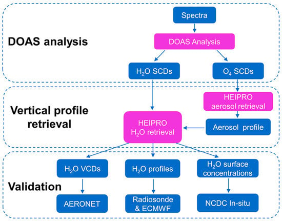
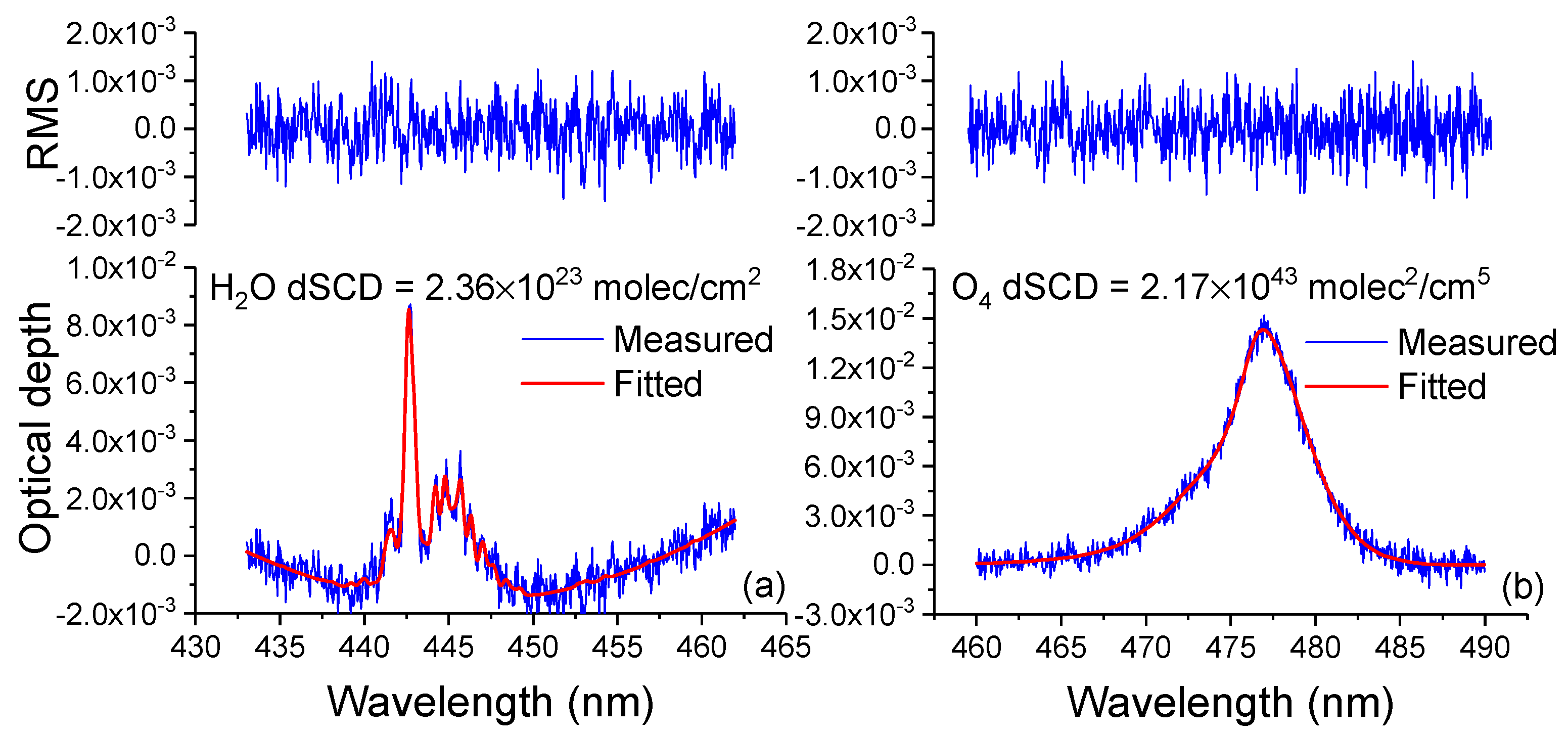
2.2. DOAS Spectral Analysis

The spectra observed in the aforementioned period were analyzed for H2O and O4 Differential Slant Column Densities (dSCDs) using the DOAS method implemented by the QDOAS software (http://uv-vis.aeronomie.be/software/QDOAS/, last access: 16 June 2020). In this step, the zenith spectrum was used as a Fraunhofer reference spectrum for each sequence to reduce the contribution of the stratospheric absorption in the derived off-axis dSCDs. Wavelength calibration was performed using a high-resolution solar spectrum [33]. The direct results retrieved from the DOAS fitting were the dSCDs, defined as the difference between the SCD for off-axis and zenith-sky measurements. These dSCDs were used as the input for the subsequent vertical profile retrieval. The dSCDs were filtered out with a Root Mean Square (RMS) larger than 0.002 or a Solar Zenith Angle (SZA) larger than 75° for quality control.
For the retrieval of H2O, an optimized fitting window of 433–462 nm and a third-order polynomial were selected via a sensitivity test (shown in Figures S2 and S3). For O4, a fitting window of 460–490 nm and a fifth-order polynomial were selected [32]. Examples of the DOAS fitting for H2O and O4 are presented in Figure 2, and the DOAS retrieval settings are listed in Table 1.

2.3. HEIPRO Algorithm Description

The Heidelberg Profile Retrieval (HEIPRO) algorithm for the vertical profiles of aerosol extinction and trace gases was used to convert the dSCDs into vertical profiles [40,41]. The universality of the HEIPRO algorithm has been demonstrated in many comparative observation experiments [42,43,44,45,46]. HEIPRO is based on a well-established optimal estimation method, which enables it to overcome the poorly constrained inversion problem [47]. The SCIATRAN 2.2 Radiative Transfer Model (RTM) [48] was used as forward model F to simulate the measurement vector y on the basis of atmospheric state vector x. The vertical profiles (both of aerosol and trace gas) were calculated iteratively by adjusting the input parameters until the optimal agreement between the measurements and RTM simulation was reached. This agreement is quantified as the minimization of the cost function χ2, which is given by the following equation (Equation (1)):
χ 2 ( x ) = [ y F ( x , b ) ] T S ε 1 [ y F ( x , b ) ] + [ x x a ] T S a 1 [ x x a ]
Here, the state vector x consists of aerosol extinction coefficients or trace gas concentrations in discrete atmospheric layers, the thicknesses of which vary from 100–200 m. The measurement vector y, which corresponds to the dSCDs in MAX-DOAS, is a function of x and the meteorological parameters b (i.e., atmospheric pressure and temperature vertical profiles). The a priori profile xa, which serves as the initial profile for profile retrieval, is iteratively used to constrain the ill-posed problem in the optimization. Sa and Sε denote the covariance matrices of a priori uncertainty and measurement error, representing the uncertainty in the a priori and measurement states, respectively.
HEIPRO implements a two-step approach to retrieve aerosol and trace gas profiles. First, aerosol extinction profiles are retrieved from the measured O4 dSCDs for each MAX-DOAS scan. Then, the retrieved aerosol extinction properties serving as the forward model parameters are combined with the measured trace gas dSCDs and used to retrieve the trace gas vertical profiles. In this study, the aerosol extinction and trace gas profiles were divided into 30 layers on a fixed altitude grid such that the first 20 layers (below 2 km) are on a 100 m grid, and the last ten layers (between 2 km and 4 km) are on a 200 m grid. The temporal interval of inversion was set to 15 min, to cover at least a full elevation sequence. For aerosol retrieval, a fixed set of aerosol properties including an asymmetry parameter of 0.72, a single scattering albedo of 0.90, and a ground albedo of 0.05 were assumed in this study [49]. An exponentially decreasing a priori profile with a surface extinction coefficient of 0.3 km−1 and a scale height of 1 km were used as a priori profiles for aerosol retrieval. The a priori uncertainty, which is used to construct Sa, was itself set as an a priori profile (relative error = 100%).
For the water vapor vertical profile retrieval, the aerosol information retrieved in the first step provides the atmospheric light path, which serves as the forward model parameter for trace gas retrieval. The overall shape of the water vapor vertical profile is determined by the Clausius–Clapeyron relationship and temperature lapse rate [30]. Thus, an exponentially decreasing a priori profile with a surface concentration of 4.6 × 10¹⁷ molec/cm3 and a scale height of 1.9 km was chosen for water vapor profile retrieval, by an exponential fitting of the ECMWF ERA-interim water vapor vertical profiles, as shown in Figure 3. Besides the a priori profile, the reasonable estimation of a priori error in each layer is important because of the large variety of profile shapes. In this paper, half of the a priori profile (relative error = 50%) was chosen as a priori uncertainty, to maintain a balance between the flexibility and stability of the profile shape [50,51].

3. Ancillary Data for Validation

The hourly averaged water vapor VCDs, surface concentrations, and vertical profiles retrieved from MAX-DOAS were validated with corresponding independent datasets. The locations of the MAX-DOAS site and other independent measurement sites are presented in Figure 1 and Table S1. The detailed data processing methods are presented in Section 5 of the supplement.
  • The MAX-DOAS water vapor VCDs were validated with AERONET Level 1.5 precipitable water data from the CAMS site, Beijing (39.933°N, 116.317°E; Elevation: 106.0 m).
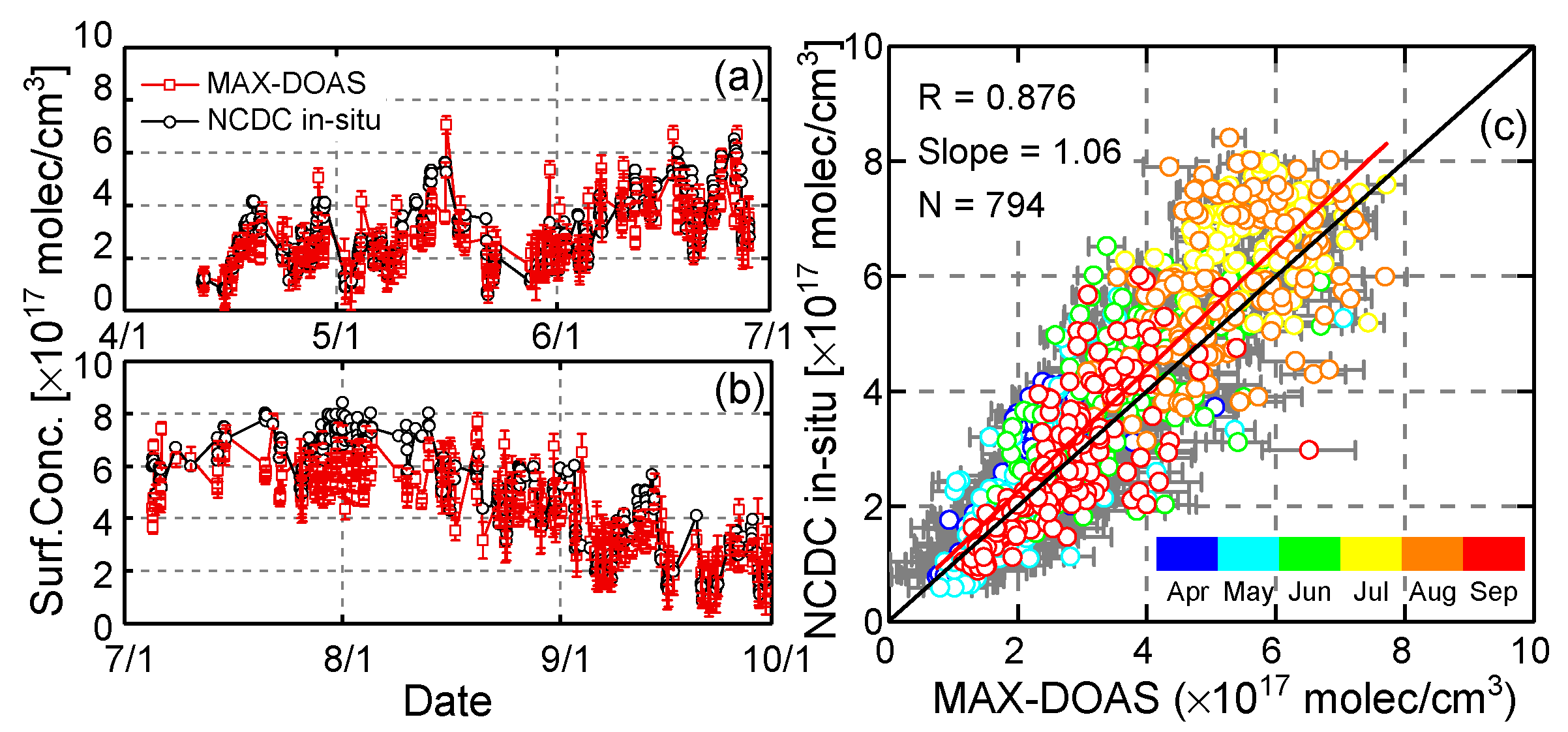
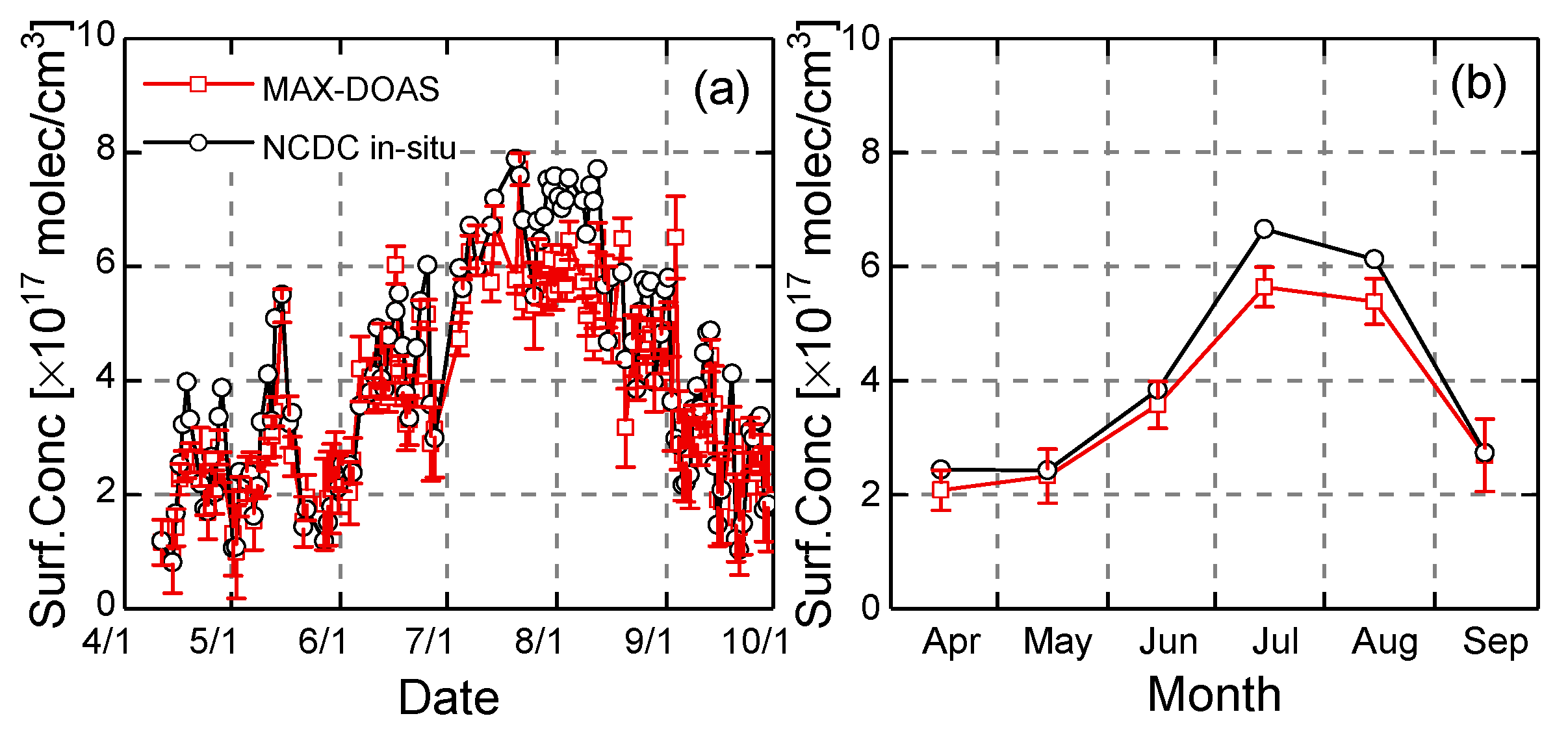
  • The MAX-DOAS water vapor surface concentrations were validated with NCDC surface meteorological data from the BCIA site (40.080°N, 116.585°E; Elevation: 35.4 m).
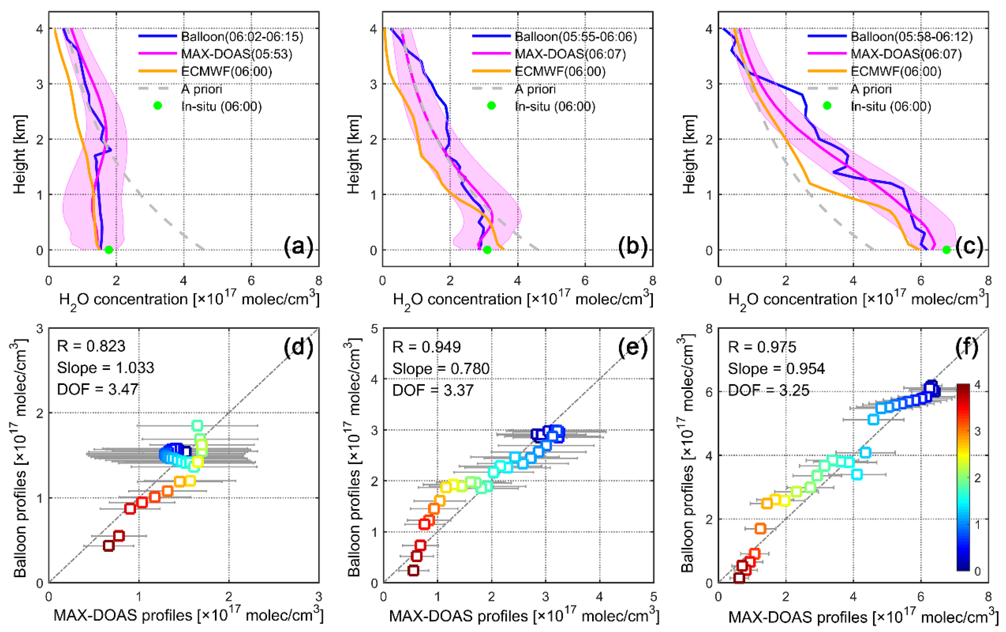
  • The MAX-DOAS water vapor vertical profiles were validated with balloon-borne radiosonde data from the Nanjiao Observatory, Beijing (39.806°N, 116.470°E) and ECMWF ERA-interim reanalysis datasets.
These validations were all performed under cloud-screened conditions, by synchronizing the timetable to that of AERONET [52]. For VCDs, any retrieved results featuring errors exceeding 1 × 10²² molec/cm2, chi-squares exceeding 100, or less than two degrees of freedom (DOFs) were further filtered out (~23% of the data). For surface concentrations, retrieved results featuring errors exceeding 1 × 10¹⁷ molec/cm3, chi-squares exceeding 100, or less than two DOFs were further filtered out (~15% of the dataset) [51]. The frequency distributions of DOFs and chi-squares can be found in Figure S4.

3.1. AERONET Observation Data

The AERONET project is a federation of ground-based Remote Sens. aerosol networks established by NASA and PHOTONS [53]. Sun photometers, as components of AERONET, not only provide information to calculate AODs but can also be used to retrieve total column water vapor quantities (water vapor VCDs) in the 940 nm channel. The AERONET data are automatically cloud screened. Thus, the absence of AERONET data often serves as a temporal index for the presence of clouds and is an external selection criterion of MAX-DOAS measurements [54,55].
In this study, the Level 1.5 precipitable water data from the Beijing-CAMS AERONET site (39.933°N, 116.317°E; Elevation: 106.0 m) were used to validate MAX-DOAS VCDs. The unit of AERONET precipitable water is the centimeter (cm), which can be converted to number density (molec/cm2) via the following relationship: 1 cm of precipitable water equals 3.3 × 10²² molec/cm2. Triplet variability values of precipitable water vapor in the AERONET data were regarded as errors of the water vapor VCDs.

3.2. NCDC Data

The hourly surface meteorological data (including temperature, pressure, dew point, wind speed, and wind direction), measured at the BCIA site (USAF ID: 545110; 40.080°N, 116.585°E; Elevation: 35.4 m) approximately 27.8 km north-east of the MAX-DOAS instrument, were obtained from the public FTP server of the NCDC (ftp://ftp.ncdc.noaa.gov/pub/data/noaa/isd-lite/, last access: 16 June 2020). The in-situ measured dew point can be converted into the molecular number density of water vapor (molec/cm3).

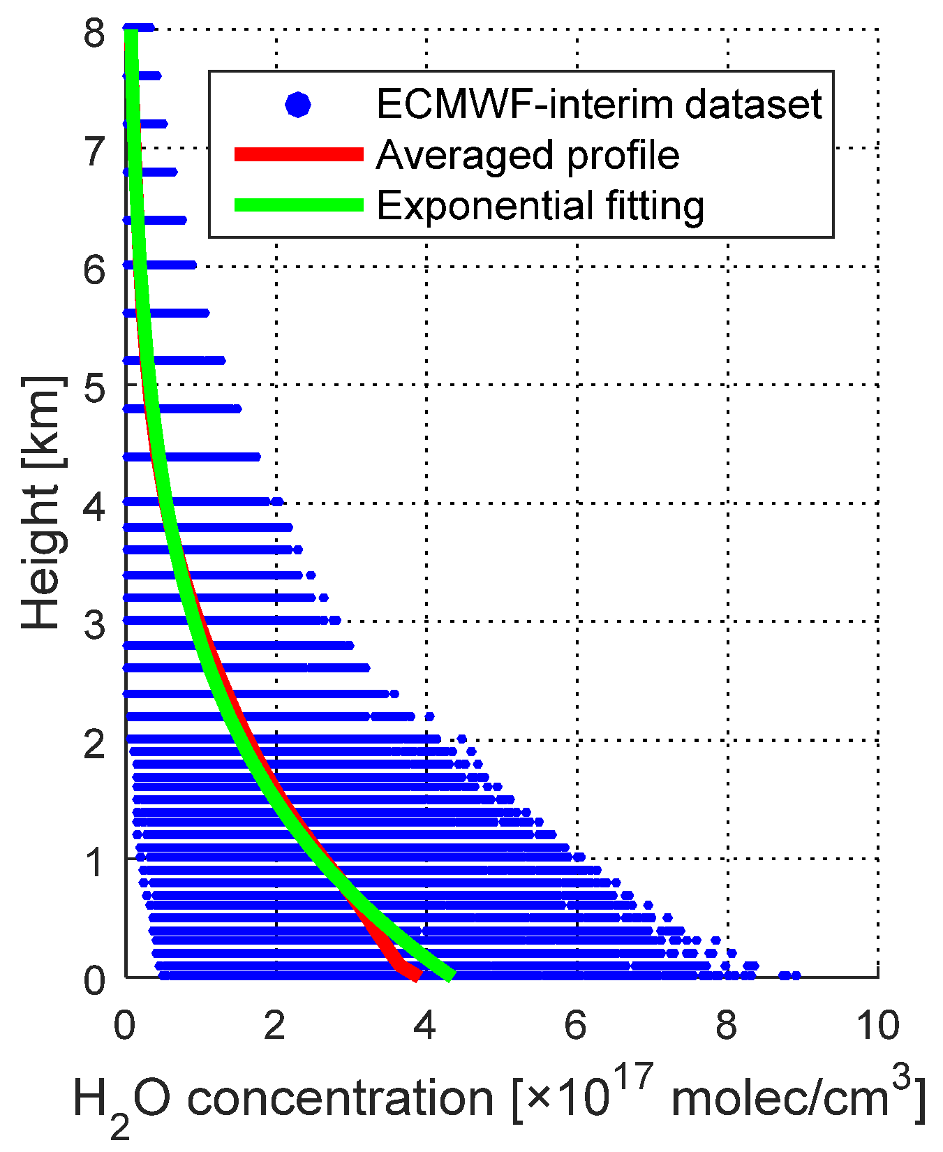
3.3. ECMWF ERA-Interim Reanalysis Data

The ECMWF ERA-interim reanalysis dataset [56] consists of a reanalysis of the global atmosphere and it is often used to validate other datasets [30,57]. In this study, the spatial and time resolutions of the ECMWF data were 0.125° × 0.125° and 6 h, respectively. The region between 39.875 and 40.0°N and between 116.25 and 116.375°E was averaged for comparison. The specific humidity in the ECMWF ERA-interim data can be converted to a number density using pressure and temperature. The pressure at each model level can be converted into height information via a barometric height formula. Thus, the vertical profiles of water vapor were illustrated by level heights and the corresponding number densities.

3.4. Balloon-Borne Radiosonde Data

Balloon-borne radiosonde measurements were conducted weekly at Nanjiao Observatory, Beijing (39.806°N, 116.470°E; Elevation = 31 m). The measurements often took place at approximately 6:00 UTC. The maximum observation height exceeded 30 km, and the temporal sampling resolution was 1 s.

4. Results

4.1. Validation of VCDs Retrieved by MAX-DOAS

The hourly averaged VCDs retrieved by MAX-DOAS were validated using AERONET Level 1.5 precipitable water data under clear sky conditions. The aerosol extinction coefficient profiles retrieved in the first step combined with meteorological profiles were used as inputs in the RTM to calculate the AMF. Thus, the dSCDs could be converted into tropospheric VCDs (denoted VCDtrop) [58], as shown in Equation (2).
VCD trop = dSCDs ( α ) AMF ( α ) AMF ( 90 )
As shown in Figure 4, the time series measurements of hourly water vapor VCDs observed by MAX-DOAS agree well with the AERONET results, achieving a high correlation coefficient R of 0.922 (number of datapoints = 739, VCDAERONET = 0.969 × VCDMAX-DOAS + 3.09 × 10²¹) through linear regression. The bias between the hourly VCDs observed by MAX-DOAS and AERONET is 5.60 × 10²¹ with a standard deviation of 1.48 × 10²². During the observation period, the hourly averaged error in the water vapor VCDs observed by MAX-DOAS ranges from 1.20 × 10²¹ to 9.89 × 10²¹, with a mean error of 4.45 × 10²¹ and a median error of 4.22 × 10²¹, while the hourly averaged error of the AERONET data ranges from 4.09 × 10¹⁹ to 2.57 × 10²² with a mean error of 2.21 × 10²¹ and a median error of 9.50 × 10²⁰. The VCD errors of AERONET measurements were smaller than those of MAX-DOAS measurements because MAX-DOAS collects solar scattering light, which is relatively weaker than the direct sunlight collected by AERONET. The AERONET results have a better precision than those of MAX-DOAS results. Here, all values are in units of molec/cm2.
As shown in Figure 5, a good agreement exists between both the daily and monthly retrieved VCDs from MAX-DOAS and AERONET. From April to July, the monthly averaged water vapor VCD derived from MAX-DOAS increased from 4.94 × 10²² ± 5.38 × 10²¹ to 1.29 × 10²³ ± 5.39 × 10²¹. Then, it decreased to 6.48 × 10²² ± 3.48 × 10²¹ in September. From April to September, the differences between the MAX-DOAS VCDs and AERONET results vary from 0.23 × 10²¹ to 0.98 × 10²¹, and the relative differences vary from 1.8% (July) to 15% (September and April). The monthly averaged VCDs of MAX-DOAS exhibit their best agreement with the AERONET results in July. All values are in units of molec/cm2.

4.2. Validation of Surface Concentrations Retrieved by MAX-DOAS

As shown in Figure 6, the hourly averaged water vapor surface concentrations observed by MAX-DOAS at the CAMS, Beijing were validated using the in-situ measurements from the BCIA under clear sky conditions. Although the distance between the two sites is more than 27 km, a good agreement (R = 0.876 and slope = 1.06) can be seen. The bias between the hourly surface concentrations measured by MAX-DOAS and NCDC in-situ instrument is −3.48 × 10¹⁶ with the standard deviation of 9.43 × 10¹⁶. The daily and monthly averaged time series results of surface concentration from MAX-DOAS and NCDC are displayed in Figure 7. The monthly averaged water vapor surface concentration retrieved from MAX-DOAS increased from 2.08 × 10¹⁷ ± 3.54 × 10¹⁶ to 5.64 × 10¹⁷ ± 3.50 × 10¹⁶ between April and July. Then, it decreased to 2.69 × 10¹⁷ ± 6.37 × 10¹⁶ in September. Here, all values are in units of molec/cm3.
The water vapor surface concentrations observed by MAX-DOAS at CAMS (urban area) are slightly lower than NCDC in-situ measurements at BCIA (suburban area), especially in July and August. This underestimation can be related to urban dryness island effect in Beijing [59]. It has been reported that the urban dryness island intensities (UDII) are high in central urban areas and the UDII is stronger in summer and autumn than in winter and spring [60]. Thus relative humidity in urban areas is smaller than in suburban areas, indicating the effect of urbanization on near-surface atmospheric moisture. This is consistent with the comparison results between MAX-DOAS and NCDC in-situ measurements.

4.3. Validations of Vertical Profiles Retrieved by MAX-DOAS

4.3.1. Validation with Balloon-Borne Radiosonde Measurements

Three representative water vapor profiles were retrieved from the MAX-DOAS measurements taken on three clear days: (a) 8 May 2018; (b) 19 June 2018; and (c) 31 July 2018; these were validated with the corresponding balloon-borne radiosonde profiles, as shown in Figure 8. The surface concentrations of these representative profiles are located in different concentration ranges. The balloon-borne radiosonde data were interpolated onto the MAX-DOAS grid for comparison. Furthermore, the interpolated ECMWF ERA-interim profiles were also used to validate the MAX-DOAS profiles. The sky conditions on 8 May 2018 and 19 June 2018 can be found in Figure S5.
The correlation analysis results for the MAX-DOAS profiles and corresponding balloon-borne radiosonde profiles are displayed in the bottom panels of Figure 8, where the colors represent the height of each layer and the horizontal gray lines indicate the errors of retrieved profile in different height layers. The biases and standard deviations between MAX-DOAS profiles and corresponding balloon-borne radiosonde profiles on 8 May 2018; 19 June 2018; and 31 July 2018 are −0.14 ± 1.78 × 10¹⁶, −0.51 ± 3.10 × 10¹⁶, and −1.10 ± 4.36 × 10¹⁶. Here, all values are in units of molec/cm3. Overall, the water vapor profiles retrieved from MAX-DOAS and radiosonde measurements exhibit a high level of consistency, with high Pearson correlation coefficients (R) for these three profiles.

4.3.2. Validation with ECMWF ERA-Interim Data

As shown in Figure 9, we conducted a correlation analysis of the water vapor concentrations in different height layers (derived from the MAX-DOAS and ECMWF ERA-interim data) to validate the profiles. As performed for the balloon-borne radiosonde measurements, the ECMWF ERA-interim water vapor profiles were also interpolated onto the MAX-DOAS grid. During this observation period, the MAX-DOAS instruments collected spectra from 00:00 to 10:00 (UTC). However, the temporal resolution of the ECMWF ERA-interim dataset is 6 h. Thus, only the MAX-DOAS profiles measured at 00:00 and 06:00 can be used to validate the corresponding ECMWF profiles. These validations were conducted under no-cloud conditions by synchronizing the timetable to the AERONET data. In total, 138 profiles measured with MAX-DOAS in this observation period from 18 April to 30 September 2018 were validated using the coincident ECMWF profiles.
Good agreement between the MAX-DOAS and ECMWF results can be observed in height layers below 2000 m, with the Pearson correlation coefficient (R) ranging from 0.695 to 0.857. Under an increase in layer height, the detection sensitivity of MAX-DOAS gradually decreases and the correlation analysis results degrade. In the layer height from 600 to 1200 m, the consistency between the MAX-DOAS concentrations and the ECMWF results is slightly worse, which may be the result of the large uncertainties in these layers. The decreasing detection sensitivity and the enhanced constraint of a priori profile together lead to the decreasing linear fitting slope with increasing height. MAX-DOAS results have high sensitivities in the lower atmosphere and the contribution of a priori profile in retrieved profile is relatively small. With the increasing height, the detection sensitivity gets worse and the dependence of retrieved profile in a priori profile becomes strong gradually. The fixed exponentially decreasing a priori profile with a surface concentration of 4.6 × 10¹⁷ molec/cm3 and a scale height of 1.9 km may be too high to represent the water vapor concentrations in high altitudes. Together with the low sensitivity in high altitudes, the retrieved concentrations in high altitudes can be higher than actual situation, thus the linear fitting slope decreases and the bias between MAX-DOAS and ECMWF increases, as shown in Figure 9.

5. Discussion

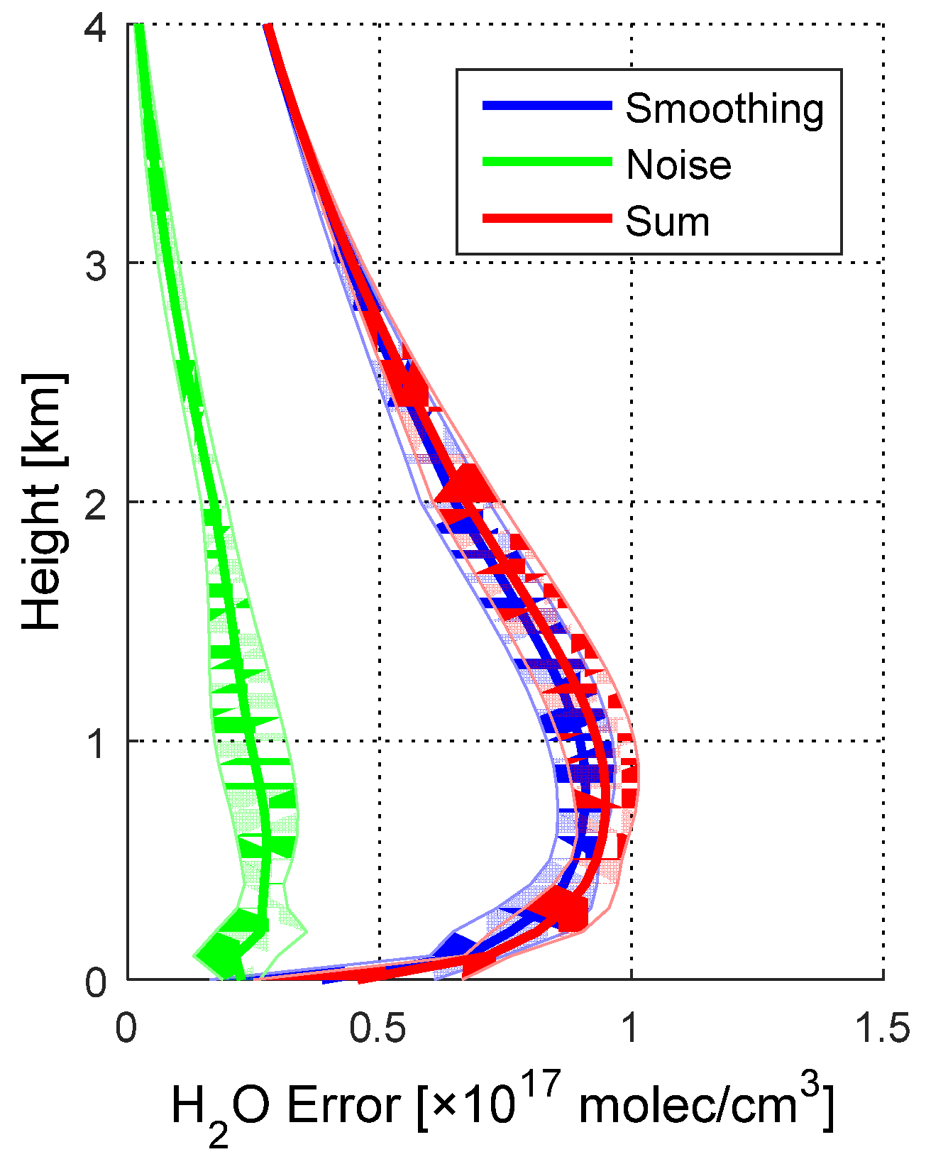
5.1. Error Budget Analysis

The errors of water vapor profile retrievals can be divided into four different types: noise error, smoothing error, model parameter error, and forward model error [61]. The noise error, defined as the fitting error of the DOAS fits, is related to the propagation of noise in the measurements inputted into the retrieval algorithm [62]. The smoothing error, which quantifies the error owing to the limited vertical resolution of profile retrieval, limits the ability of the retrieval procedure to obtain solutions from the a priori profiles. The smoothing errors Ss for the profiles are calculated from the a priori covariance matrix Sa and the averaging kernel AK [63], as shown in Equation (3).
S s = ( A K 1 ) S a ( A K 1 ) T
The model parameter errors include different parameters as aerosol profiles, cross sections and algorithm error. The forward model error originates from the simplification and uncertainties in the relative radiative model.
The algorithm error in vertical profile cannot be estimated because it is difficult to assign the discrepancies between measured and modeled dSCDs to each altitude of profiles, blocking the estimation of model parameters errors [64]. Moreover, it has been reported that the sum of smoothing error and noise error is the dominant error source in the total error budget [40,63]. The vertical distributions of the smoothing error, noise error, and the sum thereof under clear sky conditions are displayed in Figure 10. The smoothing error contributes substantially to the sum thereof, whereas the noise error has only a small influence. The smoothing and sum errors have similar vertical distributions, both increasing rapidly with height in the lower layers (0–800 m) and then decreasing gradually with height. The noise error varies marginally around 2.6 × 10¹⁶ molec/cm3 in the layers below 600 m. Then it exhibits an almost linear decrease with height.
The averaged error budgets from different sources in retrieved water vapor surface concentrations and VCDs are estimated in Table 2. Beside smoothing and noise error introduced above, the uncertainty related to aerosols is estimated by taking the retrieved aerosol profiles at 477 nm plus their corresponding errors as inputs in water vapor retrieval and then comparing the results to those of the standard retrievals [65]. The uncertainty related to the a priori profiles is estimated by comparing the retrieval results using different a priori profiles (scale height: 1.5–2.5 km; surface concentration: 3 × 10¹⁷ to 6 × 10¹⁷ molec/cm3) against the standard retrieval results. The uncertainty related to the H2O cross section is set as 3% [66]. The algorithm errors on the near-surface concentrations and the VCDs using the averaged relative differences between measured and simulated dSCDs for a 5° and 30° elevation angle, respectively [64]. The total error budgets for the surface concentrations and VCDs are calculated by adding the different error terms using Gaussian error propagation. For surface concentrations, the total uncertainty is approximately 31%, and the dominant error source is that pertaining to aerosols. However, for VCDs, the total uncertainty is approximately 38%, and the dominant error source is the sum of the smoothing and noise errors.

5.2. Retrieval Performance under Different Aerosol Loads

Aerosol loads affect the light path through which scattered photons travel, thereby determining their effective optical paths within the atmosphere [67]. Thus, in MAX-DOAS retrieval, the interpretation of trace gases strongly depends on the proper vertical distribution of the aerosol extinction coefficients [68]. As shown in Figure 11, the AOD at 477 nm (AOD477) from AERONET was divided into seven levels, and we analyzed the consistency between the MAX-DOAS results and the corresponding measurements under each AOD477 level. The root mean square error (RMSE), correlation coefficient (R), slope, and intercept of the fitted line, and the number of effective data points were selected as evaluation criteria [64].
As shown in Figure 11, aerosol loads affect the retrieval of water vapor VCDs and surface concentrations almost uniformly. Under low aerosol loads (AOD477 ≤ 1.0), the retrieved results are consistent with the corresponding measurements. The RMSEs between the MAX-DOAS results and corresponding measurements were stable and small (For VCDs, the RMSE varies in 13.92–15.98 × 10²¹ molec/cm2; for surface concentrations, the RMSE varies in 6.55–9.29 × 10¹⁶ molec/cm3). The linear fitting results were strong, with correlation coefficients (R) and fitting slopes close to 1.0, and low intercepts. Under high aerosol loads (AOD477 > 1.0), as the AOD477 increases, the consistencies degrade and the RMSEs increase almost linearly. The correlation coefficients (R) and linear fitting slopes exhibit a slight decrease, whereas the intercepts increase rapidly. The deterioration of the MAX-DOAS retrieval performance under high aerosol loads can be attributed to the more sophisticated atmosphere optical paths and lower SNRs, which obstruct the retrieval of aerosol extinction profiles in the first step. The incorrect aerosol information inputted into the water vapor retrieval procedure results in the deviation of water vapor VCDs and surface concentrations.
From the variation of RMSEs with AOD477 levels, the retrieval of surface concentrations is more strongly interfered with by aerosol loads than VCD retrieval. Interestingly, the correlation coefficient (R) and linear fitting slope also vary slightly, while the intercept of the fitting line increases rapidly under increasing AOD477 levels. In other words, a systematic deviation occurs between the MAX-DOAS results and the corresponding measurements under high aerosol loads (AOD477 > 1.0), and this deviation increases with increasing AOD477 level.

6. Summary and Conclusions

Long-term MAX-DOAS observations of water vapor in Beijing were performed from 18 April to 30 September 2018 and more than 100,000 spectra were collected. The water vapor dSCDs derived for different elevation angles were converted to VCDs, surface concentrations, and vertical profiles using the HEIPRO algorithm. The retrieved results were compared with corresponding measurements for validation.
The retrieved hourly water vapor VCDs agreed well with the AERONET data, presenting a similar temporal behavior with a correlation coefficient (R) of 0.922 and a linear fitting slope of 0.969. The retrieved hourly surface concentrations showed a good correlation with the NCDC in-situ measurements, achieving a correlation coefficient (R) of 0.876 and a fitting slope of 1.06. For the vertical profiles, the MAX-DOAS retrieved results were validated using balloon-borne radiosonde measurements from the Nanjiao Observatory, Beijing. As shown in Figure 8, three representative MAX-DOAS profiles were consistent with the corresponding balloon-borne radiosonde measurements and ECMWF ERA-interim data. Moreover, the MAX-DOAS-retrieved water vapor concentrations for different height layers (100–2000 m) were validated with the corresponding ECMWF ERA-interim datasets, with the correlation coefficient (R) varying from 0.695 to 0.857. Comparing with the previously published work [32], the consistency between the surface concentrations observed by MAX-DOAS and in-situ instrument is better, raising the Pearson correlation coefficient (R) from 0.75 to 0.876. Additionally, the retrieved vertical profile also has a higher vertical resolution. What’s more, the retrieved vertical profiles are validated using balloon-borne radiosonde measurements and ECMWF-interim datasets, which is not involved in the previous work.
Further validations were performed under different aerosol loads identified by the AERONET data. High aerosol loads obstruct the retrieval of surface concentrations and VCDs, with surface concentrations more liable to severe interference from such aerosol loads. Under low aerosol loads (AOD477 ≤ 1.0), both the surface concentrations and VCDs showed strong consistency with the corresponding measurements. Under higher aerosol loads (AOD477 > 1.0), the atmosphere optical path may become too complex to reconstruct with the HEIPRO algorithm. Thus the deterioration of the MAX-DOAS retrieval performance became evident. To summarize, the feasibility of detecting water vapor profiles using MAX-DOAS under clear sky is confirmed by this work. The retrieval under cloudy or rainy conditions is still in progress.

Supplementary Materials

Supplementary Materials are available online at https://www.mdpi.com/2072-4292/12/19/3193/s1, Figure S1: The hourly variation of surface temperature, relative humidity, and pressure; Figure S2: A test about the fitting windows of H2O SCDs; Figure S3: A test about the polynomial order in DOAS fitting; Figure S4: The normalized frequency distribution of DOFs and Chi-square in retrieved results; Figure S5: The Sky conditions on 8 May 2018 and 19 June 2018; Table S1: The information about ancillary data.

Author Contributions

Conceptualization, C.L. and Q.H. (Qihou Hu); methodology, H.L. (Hua Lin) and C.X.; software, C.X.; data curation, H.L. (Haoran Liu), Q.L., W.T., X.J. and Z.W.; writing—original draft preparation, H.L. (Hua Lin); writing—review and editing, C.X., Q.H. (Qianqian Hong) and Q.H. (Qihou Hu); project administration, C.L., Q.H. (Qihou Hu), C.X. and J.L.; funding acquisition, C.L. All authors have read and agreed to the published version of the manuscript.

Funding

This work was supported by grants from National Key Research and Development Program of China (grant nos., 2018YFC0213104, 2018YFC0213201, 2016YFC0203302, and 2017YFC0210002), Anhui Science and Technology Major Project (18030801111), the National Natural Science Foundation of China (grant nos. 41722501, 91544212, 51778596, 41575021 and 41977184), the Strategic Priority Research Program of the Chinese Academy of Sciences (grant nos. XDA23020301), the National Key Project for Causes and Control of Heavy Air Pollution (grant nos. DQGG0102-03 and DQGG0205), the National High-Resolution Earth Observation Project of China (grant nos. 05-Y30B01-9001-19/20-3), the Civil Aerospace Technology Advance Research Project, No. Y7K00100KJ and the China Postdoctoral Science Foundation (2020TQ0320).

Acknowledgments

We acknowledge the Beijing Chinese Academy of Meteorological Sciences for maintaining MAX-DOAS instrument. We thank NASA and PHOTONS for making AERONET data available online. We thank National Climate Detector Center of NOAA for offering surface meteorological data available online. We thank the ECMWF for providing access to the layered meteorological data. We thank IUP Heidelberg University to help us on HEIPRO. Besides, we would like to sincerely thank the SCIATRAN development team at the Institute of Remote Sens./Institute of Environmental Physics (IUP/IFE), University of Bremen. We also thank the Belgian Institute for Space Aeronomy (BIRAIASB), Brussels, Belgium, for their freely accessible QDOAS software.

Conflicts of Interest

The authors declare no conflict of interest.

References

  1. Moffett, K.B.; Wolf, A.; Berry, J.A.; Gorelick, S.M. Salt marsh–atmosphere exchange of energy, water vapor, and carbon dioxide: Effects of tidal flooding and biophysical controls. Water Resour. Res. 2010, 46, W10525. [Google Scholar] [CrossRef] [Green Version]
  2. Dai, A.; Wang, J.H.; Ware, R.H.; Van Hove, T. Diurnal variation in water vapor over North America and its implications for sampling errors in radiosonde humidity. J. Geophys. Res. Atmos. 2002, 107, ACL 11-1–ACL 11-14. [Google Scholar] [CrossRef] [Green Version]
  3. Chaboureau, J.P.; Chedin, A.; Scott, N.A. Remote Sens. of the vertical distribution of atmospheric water vapor from the TOVS observations: Method and validation. J. Geophys. Res. Atmos. 1998, 103, 8743–8752. [Google Scholar] [CrossRef] [Green Version]
  4. Guan, X.; Yang, L.; Zhang, Y.; Li, J. Spatial distribution, temporal variation, and transport characteristics of atmospheric water vapor over Central Asia and the arid region of China. Glob. Planet. Chang. 2019, 172, 159–178. [Google Scholar] [CrossRef]
  5. Noël, S.; Bramstedt, K.; Rozanov, A.; Bovensmann, H.; Burrows, J.P. Water vapour profiles from SCIAMACHY solar occultation measurements derived with an onion peeling approach. Atmos. Meas. Tech. 2010, 3, 523–535. [Google Scholar] [CrossRef] [Green Version]
  6. Gusakova, M.A.; Karlin, L.N. Assessment of contribution of greenhouse gases, water vapor, and cloudiness to the variations of global surface air temperature. Russ. Meteorol. Hydrol. 2014, 39, 146–151. [Google Scholar] [CrossRef]
  7. Li, L.; Tan, Q.; Zhang, Y.; Feng, M.; Qu, Y.; An, J.; Liu, X. Characteristics and source apportionment of PM2.5 during persistent extreme haze events in Chengdu, southwest China. Environ. Pollut. 2017, 230, 718–729. [Google Scholar] [CrossRef]
  8. Tie, X.; Huang, R.J.; Cao, J.; Zhang, Q.; Cheng, Y.; Su, H.; Chang, D.; Poschl, U.; Hoffmann, T.; Dusek, U.; et al. Severe Pollution in China Amplified by Atmospheric Moisture. Sci. Rep. 2017, 7, 15760. [Google Scholar] [CrossRef]
  9. Zhao, Y.; Yan, H.; Wu, P.; Zhou, D. Linear correction method for improved atmospheric vertical profile retrieval based on ground-based microwave radiometer. Atmos. Res. 2020, 232, 104678. [Google Scholar] [CrossRef]
  10. Wu, S.; Dai, G.; Song, X.; Liu, B.; Liu, L. Observations of water vapor mixing ratio profile and flux in the Tibetan Plateau based on the lidar technique. Atmos. Meas. Tech. 2016, 9, 1399–1413. [Google Scholar] [CrossRef] [Green Version]
  11. Seidel, D.J.; Sun, B.; Pettey, M.; Reale, A. Global radiosonde balloon drift statistics. J. Geophys. Res. 2011, 116, D07102. [Google Scholar] [CrossRef] [Green Version]
  12. Laroche, S.; Sarrazin, R. Impact of Radiosonde Balloon Drift on Numerical Weather Prediction and Verification. Weather Forecast. 2013, 28, 772–782. [Google Scholar] [CrossRef]
  13. Mace, G.G.; Starr, D.O.C.; Ackerman, T.P.; Minnis, P. Examination of Coupling between an Upper-Tropospheric Cloud System and Synoptic-Scale Dynamics Diagnosed from Wind Profiler and Radiosonde Data. J. Atmos. Sci. 1995, 52, 4094–4127. [Google Scholar] [CrossRef] [Green Version]
  14. Kuwagata, T.; Numaguti, A.; Endo, N. Diurnal variation of water vapor over the central Tibetan Plateau during summer. J. Meteorol. Soc. Jpn. 2001, 79, 401–418. [Google Scholar] [CrossRef] [Green Version]
  15. Bianco, L.; Friedrich, K.; Wilczak, J.M.; Hazen, D.; Wolfe, D.; Delgado, R.; Oncley, S.P.; Lundquist, J.K. Assessing the accuracy of microwave radiometers and radio acoustic sounding systems for wind energy applications. Atmos. Meas. Tech. 2017, 10, 1707–1721. [Google Scholar] [CrossRef] [Green Version]
  16. Feltz, W.F.; Smith, W.L.; Knuteson, R.O.; Revercomb, H.E.; Woolf, H.M.; Howell, H.B. Meteorological Applications of Temperature and Water Vapor Retrievals from the Ground-Based Atmospheric Emitted Radiance Interferometer (AERI). J. Appl. Meteorol. 1998, 37, 857–875. [Google Scholar] [CrossRef]
  17. Löhnert, U.; Turner, D.D.; Crewell, S. Ground-Based Temperature and Humidity Profiling Using Spectral Infrared and Microwave Observations. Part I: Simulated Retrieval Performance in Clear-Sky Conditions. J. Appl. Meteorol. Climatol. 2009, 48, 1017–1032. [Google Scholar] [CrossRef]
  18. Roy, R.J.; Lebsock, M.; Millan, L.; Dengler, R.; Monje, R.R.; Siles, J.V.; Cooper, K.B. Boundary-layer water vapor profiling using differential absorption radar. Atmos. Meas. Tech. 2018, 11, 6511–6523. [Google Scholar] [CrossRef] [Green Version]
  19. Ehret, G.; Hoinka, K.P.; Stein, J.; Fix, A.; Kiemle, C.; Poberaj, G. Low stratospheric water vapor measured by an airborne DIAL. J. Geophys. Res. Atmos. 1999, 104, 31351–31359. [Google Scholar] [CrossRef]
  20. Browell, E.V.; Wilkerson, T.D.; McIlrath, T.J. Water vapor differential absorption lidar development and evaluation. Appl. Opt. 1979, 18, 3474–3483. [Google Scholar] [CrossRef]
  21. Whiteman, D.N.; Melfi, S.H.; Ferrare, R.A. Raman lidar system for the measurement of water vapor and aerosols in the Earth’s atmosphere. Appl. Opt. 1992, 31, 3068–3082. [Google Scholar] [CrossRef] [PubMed]
  22. Weber, K.J.; Weckwerth, T.M.; Turner, D.D.; Spuler, S.M. Validation of a Water Vapor Micropulse Differential Absorption Lidar (DIAL). J. Atmos. Ocean. Technol. 2016, 33, 2353–2372. [Google Scholar] [CrossRef]
  23. Honninger, G.; von Friedeburg, C.; Platt, U. Multi axis differential optical absorption spectroscopy (MAX-DOAS). Atmos. Chem. Phys. 2004, 4, 231–254. [Google Scholar] [CrossRef] [Green Version]
  24. Li, X.; Brauers, T.; Hofzumahaus, A.; Lu, K.; Li, Y.P.; Shao, M.; Wagner, T.; Wahner, A. MAX-DOAS measurements of NO2, HCHO and CHOCHO at a rural site in Southern China. Atmos. Chem. Phys. 2013, 13, 2133–2151. [Google Scholar] [CrossRef] [Green Version]
  25. Xing, C.Z.; Liu, C.; Wang, S.S.; Hu, Q.H.; Liu, H.R.; Tan, W.; Zhang, W.Q.; Li, B.; Liu, J.G. A new method to determine the aerosol optical properties from multiple-wavelength O4 absorptions by MAX-DOAS observation. Atmos. Meas. Tech. 2019, 12, 3289–3302. [Google Scholar] [CrossRef] [Green Version]
  26. Cheng, Y.; Wang, S.; Zhu, J.; Guo, Y.; Zhang, R.; Liu, Y.; Zhang, Y.; Yu, Q.; Ma, W.; Zhou, B. Surveillance of SO2 and NO2 from ship emissions by MAX-DOAS measurements and the implications regarding fuel sulfur content compliance. Atmos. Chem. Phys. 2019, 19, 13611–13626. [Google Scholar] [CrossRef] [Green Version]
  27. Suwen, L.; Fusheng, M.; Jing, L.; Wen, S.; Minhong, W.; Xude, W.; Lisha, H. Research of vertical profile of aerosol extinction based on measured the O4 of multi-elevation angles with MAX-DOAS. In Proceedings of the Optical Sensors and Sensing Congress (ES, FTS, HISE, Sensors), San Jose, CA, USA, 25–27 June 2019; p. JW3A-13. [Google Scholar]
  28. Javed, Z.; Liu, C.; Khokhar, M.F.; Tan, W.; Liu, H.R.; Xing, C.Z.; Ji, X.G.; Tanvir, A.; Hong, Q.Q.; Sandhu, O.; et al. Ground-Based MAX-DOAS Observations of CHOCHO and HCHO in Beijing and Baoding, China. Remote Sens. 2019, 11, 1524. [Google Scholar] [CrossRef] [Green Version]
  29. Zhang, J.; Wang, S.; Guo, Y.; Zhang, R.; Qin, X.; Huang, K.; Wang, D.; Fu, Q.; Wang, J.; Zhou, B. Aerosol vertical profile retrieved from ground-based MAX-DOAS observation and characteristic distribution during wintertime in Shanghai, China. Atmos. Environ. 2018, 192, 193–205. [Google Scholar] [CrossRef] [Green Version]
  30. Wagner, T.; Andreae, M.O.; Beirle, S.; Dörner, S.; Mies, K.; Shaiganfar, R. MAX-DOAS observations of the total atmospheric water vapour column and comparison with independent observations. Atmos. Meas. Tech. 2013, 6, 131–149. [Google Scholar] [CrossRef] [Green Version]
  31. Baidar, S.; Oetjen, H.; Coburn, S.; Dix, B.; Ortega, I.; Sinreich, R.; Volkamer, R. The CU Airborne MAX-DOAS instrument: Vertical profiling of aerosol extinction and trace gases. Atmos. Meas. Tech. 2013, 6, 719–739. [Google Scholar] [CrossRef] [Green Version]
  32. Irie, H.; Takashima, H.; Kanaya, Y.; Boersma, K.F.; Gast, L.; Wittrock, F.; Brunner, D.; Zhou, Y.; Van Roozendael, M. Eight-component retrievals from ground-based MAX-DOAS observations. Atmos. Meas. Tech. 2011, 4, 1027–1044. [Google Scholar] [CrossRef] [Green Version]
  33. Chance, K.; Kurucz, R.L. An improved high-resolution solar reference spectrum for earth’s atmosphere measurements in the ultraviolet, visible, and near infrared. J. Quant. Spectrosc. Radiat. Transf. 2010, 111, 1289–1295. [Google Scholar] [CrossRef]
  34. Vandaele, A.C.; Hermans, C.; Simon, P.C.; Carleer, M.; Colin, R.; Fally, S.; Merienne, M.F.; Jenouvrier, A.; Coquart, B. Measurements of the NO2 absorption cross-section from 42 000 cm−1 to 10 000 cm−1 (238–1000 nm) at 220 K and 294 K. J. Quant. Spectrosc. Radiat. Transf. 1998, 59, 171–184. [Google Scholar] [CrossRef] [Green Version]
  35. Thalman, R.; Volkamer, R. Temperature dependent absorption cross-sections of O2-O2 collision pairs between 340 and 630 nm and at atmospherically relevant pressure. Phys. Chem. Chem. Phys. 2013, 15, 15371–15381. [Google Scholar] [CrossRef]
  36. Serdyuchenko, A.; Gorshelev, V.; Weber, M.; Chehade, W.; Burrows, J.P. High spectral resolution ozone absorption cross-sections—Part 2: Temperature dependence. Atmos. Meas. Tech. 2014, 7, 625–636. [Google Scholar] [CrossRef] [Green Version]
  37. Volkamer, R.; Spietz, P.; Burrows, J.; Platt, U. High-resolution absorption cross-section of glyoxal in the UV-vis and IR spectral ranges. J. Photochem. Photobiol. A Chem. 2005, 172, 35–46. [Google Scholar] [CrossRef]
  38. Rothman, L.S.; Gordon, I.E.; Barbe, A.; Benner, D.C.; Bernath, P.E.; Birk, M.; Boudon, V.; Brown, L.R.; Campargue, A.; Champion, J.P.; et al. The HITRAN 2008 molecular spectroscopic database. J. Quant. Spectrosc. Radiat. Transf. 2009, 110, 533–572. [Google Scholar] [CrossRef] [Green Version]
  39. Chance, K.V.; Spurr, R.J.D. Ring effect studies: Rayleigh scattering, including molecular parameters for rotational Raman scattering, and the Fraunhofer spectrum. Appl. Opt. 1997, 36, 5224–5230. [Google Scholar] [CrossRef] [Green Version]
  40. Frieß, U.; Monks, P.S.; Remedios, J.J.; Rozanov, A.; Sinreich, R.; Wagner, T.; Platt, U. MAX-DOAS O4 measurements: A new technique to derive information on atmospheric aerosols: 2. Modeling studies. J. Geophys. Res. 2006, 111, D14203. [Google Scholar] [CrossRef] [Green Version]
  41. Wagner, T.; Dix, B.; Friedeburg, C.v.; Frieß, U.; Sanghavi, S.; Sinreich, R.; Platt, U. MAX-DOAS O4 measurements: A new technique to derive information on atmospheric aerosols—Principles and information content. J. Geophys. Res. Atmos. 2004, 109, D22205. [Google Scholar] [CrossRef] [Green Version]
  42. Frieß, U.; Klein Baltink, H.; Beirle, S.; Clémer, K.; Hendrick, F.; Henzing, B.; Irie, H.; de Leeuw, G.; Li, A.; Moerman, M.M.; et al. Intercomparison of aerosol extinction profiles retrieved from MAX-DOAS measurements. Atmos. Meas. Tech. 2016, 9, 3205–3222. [Google Scholar] [CrossRef] [Green Version]
  43. Ryan, R.G.; Rhodes, S.; Tully, M.; Wilson, S.; Jones, N.; Friess, U.; Schofield, R. Daytime HONO, NO2 and aerosol distributions from MAX-DOAS observations in Melbourne. Atmos. Chem. Phys. 2018, 18, 13969–13985. [Google Scholar] [CrossRef] [Green Version]
  44. Wang, S.; Cuevas, C.A.; Frieß, U.; Saiz-Lopez, A. MAX-DOAS retrieval of aerosol extinction properties in Madrid, Spain. Atmos. Meas. Tech. 2016, 9, 5089–5101. [Google Scholar] [CrossRef] [Green Version]
  45. Xing, C.; Liu, C.; Wang, S.; Chan, K.L.; Gao, Y.; Huang, X.; Su, W.; Zhang, C.; Dong, Y.; Fan, G.; et al. Observations of the vertical distributions of summertime atmospheric pollutants and the corresponding ozone production in Shanghai, China. Atmos. Chem. Phys. 2017, 17, 14275–14289. [Google Scholar] [CrossRef] [Green Version]
  46. Xing, C.Z.; Liu, C.; Hu, Q.H.; Fu, Q.Y.; Lin, H.; Wang, S.T.; Su, W.J.; Wang, W.W.; Javed, Z.; Liu, J.G. Identifying the wintertime sources of volatile organic compounds (VOCs) from MAX-DOAS measured formaldehyde and glyoxal in Chongqing, southwest China. Sci. Total Environ. 2020, 715, 136258. [Google Scholar] [CrossRef]
  47. Frieß, U.; Beirle, S.; Alvarado Bonilla, L.; Bösch, T.; Friedrich, M.M.; Hendrick, F.; Piters, A.; Richter, A.; van Roozendael, M.; Rozanov, V.V.; et al. Intercomparison of MAX-DOAS Vertical Profile Retrieval Algorithms: Studies using Synthetic Data. Atmos. Meas. Tech. Discuss. 2018. [Google Scholar] [CrossRef]
  48. Rozanov, V.V.; Rozanov, A.V.; Kokhanovsky, A.A.; Burrows, J.P. Radiative transfer through terrestrial atmosphere and ocean: Software package SCIATRAN. J. Quant. Spectrosc. Radiat. Transf. 2014, 133, 13–71. [Google Scholar] [CrossRef]
  49. Ma, J.Z.; Beirle, S.; Jin, J.L.; Shaiganfar, R.; Yan, P.; Wagner, T. Tropospheric NO2 vertical column densities over Beijing: Results of the first three years of ground-based MAX-DOAS measurements (2008–2011) and satellite validation. Atmos. Chem. Phys. 2013, 13, 1547–1567. [Google Scholar] [CrossRef] [Green Version]
  50. Schofield, R.; Connor, B.; Kreher, K.; Johnston, P.; Rodgers, C. The retrieval of profile and chemical information from ground-based UV-visible spectroscopic measurements. J. Quant. Spectrosc. Radiat. Transf. 2004, 86, 115–131. [Google Scholar] [CrossRef]
  51. Vlemmix, T.; Hendrick, F.; Pinardi, G.; De Smedt, I.; Fayt, C.; Hermans, C.; Piters, A.; Wang, P.; Levelt, P.; Van Roozendael, M. MAX-DOAS observations of aerosols, formaldehyde and nitrogen dioxide in the Beijing area: Comparison of two profile retrieval approaches. Atmos. Meas. Tech. 2015, 8, 941–963. [Google Scholar] [CrossRef] [Green Version]
  52. Chan, K.L.; Wang, Z.; Ding, A.; Heue, K.-P.; Shen, Y.; Wang, J.; Zhang, F.; Shi, Y.; Hao, N.; Wenig, M. MAX-DOAS measurements of tropospheric NO2 and HCHO in Nanjing and a comparison to ozone monitoring instrument observations. Atmos. Chem. Phys. 2019, 19, 10051–10071. [Google Scholar] [CrossRef] [Green Version]
  53. Holben, B.N.; Eck, T.F.; Slutsker, I.; Tanre, D.; Buis, J.P.; Setzer, A.; Vermote, E.; Reagan, J.A.; Kaufman, Y.J.; Nakajima, T.; et al. AERONET—A federated instrument network and data archive for aerosol characterization. Remote Sens. Environ. 1998, 66, 1–16. [Google Scholar] [CrossRef]
  54. Smirnov, A.; Holben, B.N.; Eck, T.F.; Dubovik, O.; Slutsker, I. Cloud-Screening and Quality Control Algorithms for the AERONET Database. Remote Sens. Environ. 2000, 73, 337–349. [Google Scholar] [CrossRef]
  55. Hoque, H.M.S.; Irie, H.; Damiani, A.; Momoi, M. Primary Evaluation of the GCOM-C Aerosol Products at 380 nm Using Ground-Based Sky Radiometer Observations. Remote Sens. 2020, 12, 2661. [Google Scholar] [CrossRef]
  56. Dee, D.P.; Uppala, S.M.; Simmons, A.J.; Berrisford, P.; Poli, P.; Kobayashi, S.; Andrae, U.; Balmaseda, M.A.; Balsamo, G.; Bauer, P.; et al. The ERA-Interim reanalysis: Configuration and performance of the data assimilation system. Q. J. R. Meteorol. Soc. 2011, 137, 553–597. [Google Scholar] [CrossRef]
  57. Yao, Y.; Xin, L.; Zhao, Q. An improved pixel-based water vapor tomography model. Ann. Geophys. 2019, 37, 89–100. [Google Scholar] [CrossRef] [Green Version]
  58. Tan, W.; Liu, C.; Wang, S.; Xing, C.; Su, W.; Zhang, C.; Xia, C.; Liu, H.; Cai, Z.; Liu, J. Tropospheric NO2, SO2, and HCHO over the East China Sea, using ship-based MAX-DOAS observations and comparison with OMI and OMPS satellite data. Atmos. Chem. Phys. 2018, 18, 15387–15402. [Google Scholar] [CrossRef] [Green Version]
  59. Wang, X.; Gong, Y. The impact of an urban dry island on the summer heat wave and sultry weather in Beijing City. Chin.Sci. Bull. 2010, 55, 1657–1661. [Google Scholar] [CrossRef]
  60. Yang, P.; Ren, G.; Hou, W. Temporal–Spatial Patterns of Relative Humidity and the Urban Dryness Island Effect in Beijing City. J. Appl. Meteorol. Climatol. 2017, 56, 2221–2237. [Google Scholar] [CrossRef]
  61. Rodgers, C. Inverse Methods for Atmospheric Sounding: Theory and Practice, Series on Atmospheric, Oceanic and Planetary Physics; World Scientific Publishing Co.: Singapore, 2000. [Google Scholar] [CrossRef]
  62. Hong, Q.Q.; Liu, C.; Hu, Q.H.; Xing, C.Z.; Tan, W.; Liu, H.R.; Huang, Y.; Zhu, Y.; Zhang, J.S.; Geng, T.Z.; et al. Evolution of the vertical structure of air pollutants during winter heavy pollution episodes: The role of regional transport and potential sources. Atmos. Res. 2019, 228, 206–222. [Google Scholar] [CrossRef]
  63. Friedrich, M.M.; Rivera, C.; Stremme, W.; Ojeda, Z.; Arellano, J.; Bezanilla, A.; García-Reynoso, J.A.; Grutter, M. NO2 vertical profiles and column densities from MAX-DOAS measurements in Mexico City. Atmos. Meas. Tech. 2019, 12, 2545–2565. [Google Scholar] [CrossRef] [Green Version]
  64. Wang, Y.; Lampel, J.; Xie, P.; Beirle, S.; Li, A.; Wu, D.; Wagner, T. Ground-based MAX-DOAS observations of tropospheric aerosols, NO2, SO2 and HCHO in Wuxi, China, from 2011 to 2014. Atmos. Chem. Phys. 2017, 17, 2189–2215. [Google Scholar] [CrossRef] [Green Version]
  65. Wang, T.; Hendrick, F.; Wang, P.; Tang, G.; Clemer, K.; Yu, H.; Fayt, C.; Hermans, C.; Gielen, C.; Muller, J.F.; et al. Evaluation of tropospheric SO2 retrieved from MAX-DOAS measurements in Xianghe, China. Atmos. Chem. Phys. 2014, 14, 11149–11164. [Google Scholar] [CrossRef] [Green Version]
  66. Wagner, T.; Heland, J.; Zoger, M.; Platt, U. A fast H2O total column density product from GOME—Validation with in-situ aircraft measurements. Atmos. Chem. Phys. 2003, 3, 651–663. [Google Scholar] [CrossRef] [Green Version]
  67. Chan, K.L.; Hartl, A.; Lam, Y.F.; Xie, P.H.; Liu, W.Q.; Cheung, H.M.; Lampel, J.; Poehler, D.; Li, A.; Xu, J.; et al. Observations of tropospheric NO2 using ground based MAX-DOAS and OMI measurements during the Shanghai World Expo 2010. Atmos. Environ. 2015, 119, 45–58. [Google Scholar] [CrossRef]
  68. Garcia-Nieto, D.; Benavent, N.; Saiz-Lopez, A. Measurements of atmospheric HONO vertical distribution and temporal evolution in Madrid (Spain) using the MAX-DOAS technique. Sci. Total Environ. 2018, 643, 957–966. [Google Scholar] [CrossRef]
Figure 1. Location of the measurement sites in Beijing. The Multi-Axis Differential Optical Absorption Spectroscopy (MAX-DOAS) and Aerosol Robotic Network (AERONET) instruments are collocated at the CAMS, Beijing. The National Oceanic and Atmospheric Administration-NCDC in-situ instrument collects surface humidity measurements at Beijing Capital International Airport (BCIA). The balloon-borne radiosonde measurements are conducted weekly at Nanjiao Observatory, Beijing.
Remotesensing 12 03193 g001
Figure 2. Spectral proofs for the detection of H2O (a) and O4 (b) at 07:48 UTC (SZA: ~47.2°) with an elevation angle of 10° on 19 June 2018. The blue and red lines represent the measured spectra and the fitted reference cross sections, respectively.
Remotesensing 12 03193 g002
Figure 3. Determination of a priori profiles in Heidelberg Profile Retrieval (HEIPRO) using European Centre for Medium-range Weather Forecasts (ECMWF) ERA-interim reanalysis datasets. The blue points represent interpolated water vapor profiles from the ECMWF ERA-interim datasets between 12 April and 30 September 2018. The red and green lines represent the averaged ECMWF ERA-interim profile and exponential fitting profile, respectively.
Remotesensing 12 03193 g003
Figure 4. Comparison of the hourly averaged water vapor Vertical Column Densities (VCDs) retrieved from MAX-DOAS and AERONET. Panels (a,b) show two segments of the measurement time series (12 April–30 June 2018; 1 July–30 September 2018) of the hourly averaged water vapor VCDs derived from MAX-DOAS and AERONET. Panel (c) shows the correlation analysis of hourly averaged water vapor VCDs from MAX-DOAS and AERONET. All values are in units of molec/cm2.
Remotesensing 12 03193 g004
Figure 5. The daily (a) and monthly (b) averaged time series of water vapor VCDs retrieved from MAX-DOAS and AERONET.
Remotesensing 12 03193 g005
Figure 6. Hourly averaged water vapor surface concentrations retrieved from MAX-DOAS, compared with NCDC in-situ measurements. The variation of water vapor surface concentration from MAX-DOAS and NCDC in two time series: (a) 12 April–30 June 2018; (b) 1 July–30 September 2018. Panel (c) displays the correlations between them. Colors represent the months of the observation period.
Remotesensing 12 03193 g006
Figure 7. Daily (a) and monthly (b) averaged time series of water vapor surface concentrations derived from MAX-DOAS and NCDC.
Remotesensing 12 03193 g007
Figure 8. Three typical water vapor profiles retrieved from MAX-DOAS with the corresponding balloon-borne radiosonde measurements, ECMWF ERA-interim datasets, and NCDC in-situ measurements taken on 8 May 2018 (a); 19 June 2018 (b); and 31 July 2018 (c). The blue lines represent the water vapor concentration profiles measured by balloon-borne radiosonde. The pink lines and the shaded areas represent the MAX-DOAS retrieved water vapor profiles and their errors. The orange lines represent the water vapor profiles derived from the ECMWF ERA-interim reanalysis dataset. The dashed gray lines represent the a priori profile used in water vapor profile retrieval. The green dots represent the surface concentration of water vapor measured by the NCDC in-situ instruments. The bottom panels display the corresponding correlation analysis results between the MAX-DOAS-retrieved and radiosonde water vapor profiles on 8 May 2018 (d); 19 June 2018 (e); and 31 July 2018 (f), where colors indicate the height of each layer and the horizontal gray lines indicate the errors of retrieved profile in different height layers.
Remotesensing 12 03193 g008
Figure 9. Correlation analysis of MAX-DOAS water vapor concentrations and ECMWF results in different the MAX-DOAS grid using a linear method to facilitate vertical layers. The 00:00 and 06:00 UTC ECMWF profiles are interpolated onto the comparison. Both the MAX-DOAS and ECMWF profiles are normalized to the AERONET timetable for cloud screening. The Pearson correlation coefficient (R), linear fitting slope (Slope), the bias with stand deviation (SD) between MAX-DOAS and ECMWF result at each layer are given in this figure. All values here are in units of 1017 molec/cm2.
Remotesensing 12 03193 g009
Figure 10. Averaged vertical distributions of noise error (green), smoothing error (blue), and the sum thereof (red) during the measurement period.
Remotesensing 12 03193 g010
Figure 11. (a) Validation results for MAX-DOAS VCDs with AERONET measurements under different AOD levels. The root mean square errors (RMSEs) calculated from the two datasets, correlation coefficients (R), slopes, and intercepts derived using linear regression, and the corresponding numbers of data points under different aerosol optical depth (AOD) levels are displayed as red dots. (b) As (a), but for the correlation between surface concentrations retrieved from MAX-DOAS and NCDC in-situ instruments.
Remotesensing 12 03193 g011
Table 1. DOAS retrieval settings for O4 and H2O.
ParametersData SourceTarget Component
H2OO4
Fitting window 433–462 nm460–490 nm
NO2298 K [34]
NO2220 K [34]
O4293 K [35]
O3223 K [36]
Glyoxal298 K [37]
H2O293 K, 1021 hPa [38]
RingCalculated with QDOAS [39]
Polynomial degree 3rd order5th order
Intensity offset ConstantConstant
Table 2. Averaged error budget of retrieved water vapor surface concentrations and VCDs.
UncertaintySurf. Concentration (0–100 m)VCD
Smoothing and noise error13%36%
Uncertainty related to aerosols28%5%
Uncertainty related to a priori profile2%7%
Uncertainty in H2O cross section3%3%
Algorithm error1%8%
Total error31%38%

