Cloud Detection of SuperView-1 Remote Sensing Images Based on Genetic Reinforcement Learning

Abstract

Cloud pixels have massively reduced the utilization of optical remote sensing images, highlighting the importance of cloud detection. According to the current remote sensing literature, methods such as the threshold method, statistical method and deep learning (DL) have been applied in cloud detection tasks. As some cloud areas are translucent, areas blurred by these clouds still retain some ground feature information, which blurs the spectral or spatial characteristics of these areas, leading to difficulty in accurate detection of cloud areas by existing methods. To solve the problem, this study presents a cloud detection method based on genetic reinforcement learning. Firstly, the factors that directly affect the classification of pixels in remote sensing images are analyzed, and the concept of pixel environmental state (PES) is proposed. Then, PES information and the algorithm’s marking action are integrated into the “PES-action” data set. Subsequently, the rule of “reward–penalty” is introduced and the “PES-action” strategy with the highest cumulative return is learned by a genetic algorithm (GA). Clouds can be detected accurately through the learned “PES-action” strategy. By virtue of the strong adaptability of reinforcement learning (RL) to the environment and the global optimization ability of the GA, cloud regions are detected accurately. In the experiment, multi-spectral remote sensing images of SuperView-1 were collected to build the data set, which was finally accurately detected. The overall accuracy (OA) of the proposed method on the test set reached 97.15%, and satisfactory cloud masks were obtained. Compared with the best DL method disclosed and the random forest (RF) method, the proposed method is superior in precision, recall, false positive rate (FPR) and OA for the detection of clouds. This study aims to improve the detection of cloud regions, providing a reference for researchers interested in cloud detection of remote sensing images.

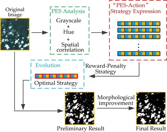
1. Introduction

With advantages of large coverage, strong time validity and favorable data geographical integration [1,2,3,4,5], satellite remote sensing images are increasingly employed in various aspects, such as Earth resource surveys, natural disaster forecasts, environmental pollution monitoring, climate change monitoring and ground target recognition. However, these tasks are vulnerable to a large amount of cloud in remote sensing images [6,7,8,9]. Although accurate cloud masks can be created manually, it is time-consuming; therefore, accurate automatic cloud detection should be prioritized during the processing of remote sensing images.

Although cloud detection technology has undergone considerable improvement, there are still some problems that have not yet been resolved in such fields that require accurate detection of cloud regions. Multi-temporal cloud detection algorithms are reported to have higher accuracy than single-date cloud detection algorithms in most cases, yet their applications are limited by necessary clear sky reference images and high-density time series data, while with simple input image requirements, single-date cloud detection algorithms have wider practical applications. Generally, in terms of optical remote sensing images, the single-date cloud detection algorithm mainly focuses on the physical method using spectral reflection characteristics, the texture statistical method and machine learning.

Due to the different spectral reflection characteristics of cloud and ground, the reflectivity of cloud is higher than that of ground features such as vegetation, water and soil in visible wavelengths. Physical methods usually distinguish cloud pixels from other pixels by thresholds, which depend on the corresponding reflective properties of cloud and ground. Although a single global threshold is simple and easy to implement, it has accuracy flaws; therefore, a dual-spectral threshold detection method for cloud detection using the spectral characteristics of visible and infrared channels was proposed by Raynolds and Haar [10]. As the satellite camera technology has improved, multi-threshold technology has been promoted by multi-spectral images. A series of physical thresholds was used by Saunders to process the data from an advanced very high-resolution radar (AVHRR) sensor [11]. Later, the automatic cloud coverage assessment (ACCA) algorithm adopted multiple band information of Landsat7 ETM+ to obtain cloud mask products [12,13]. Subsequently, the function of mask (Fmask) algorithm developed for Landsat series and Sentinel-2 satellite imagery took almost all the available band information (viewed as an extension of ACCA) [14,15,16]. Although physical methods have the advantages of simple models and fast computing speed, their accuracy is curtailed by the translucent clouds and cloud-like ground features in remote sensing images. In particular, ACCA and Fmask algorithms require enough spectral information for support, and the remote sensing data with insufficient spectrum bands are not qualified.

Due to the complexity of cloud and ground information in remote sensing images, cloud is difficult detect accurately merely through spectral characteristics, thus cloud detection algorithms based on cloud textures and spatial information have been developed. Since the spatial information between pixels displays the structure properties of the object, it is consistent with human visual observation [17]. The type of texture is distinguished by virtue of the pattern and spatial distribution of the textures, achieving classification of cloud and ground [18]. Energy, entropy, contrast, reciprocal difference distance, correlation and other feature criteria derived from the gray level co-occurrence matrix were used to target the image texture characteristics in 1988 [19]. In [20], a cloud detection method based on fractal dimension variance was presented. An effective way of extracting multi-scale spatial features is provided by the introduction of wavelet transform, expressing texture features in different resolutions and improving the accuracy of cloud detection [21]. Although the accuracy of cloud detection is improved by the method based on texture statistics, these methods are complicated and time-consuming. As the features such as image contrast and fractal dimension are mainly designed manually, and some cloud feathers are similar to ground features, discrimination errors are possible and method generalization not guaranteed.

To facilitate the generalization of cloud detection algorithms and avoid manual design features, machine learning technologies that can automatically learn features are widely adopted in cloud detection tasks [22,23], including artificial neural networks [24,25], support vector machines (SVMs) [26,27,28], clustering [29,30], RF [31,32], DL [33,34,35,36,37,38], and so forth. As computer technology thrives, cloud detection algorithms based on DL have become a research hotspot. A remote sensing network (RS-net) based on the u-net structure for cloud detection was proposed by Jeppesen et al. [39]. In [40], multi-scale information was fused into convolution features and a multi-scale convolutional feature fusion (MSCFF) cloud detection method was put forward. Cloud features can be automatically extracted by DL methods and human intervention minimized through model self-learning, but a huge data set is required by DL methods to learn, which is currently difficult to achieve. Moreover, due to the cloud regions’ unstable shape, random size and complexity, a pooling operation is inevitable, and the DL method is thus not precise enough for detection of the complex cloud edge.

In terms of the existing cloud detection methods, including physical method, texture statistical method and DL method, the accurate detection of cloud fails to materialize. Cloud with obvious features can be detected accurately by most cloud detection algorithms. Yet some clouds tend to attenuate the signal collected by the optical sensor, though it is not completely blocked. The pixels blurred by these clouds still retain some ground spectral information, increasing the difficulty of detection. Translucent clouds exist in almost all the cloud images. The most important factor undermining the accuracy of cloud detection is translucent cloud. It is noteworthy that the point is the degree of occlusion of the ground by cloud, rather than the geometric thickness of cloud. During satellite imagery acquisition, the energy received by its sensors comes from the sun. The sun’s atomic radiation first refracts and scatters within the Earth’s atmosphere, then bounces off the Earth’s surface, refracts and scatters again within the Earth’s atmosphere, and finally reaches the sensor. Clouds are clusters of small water droplets or (and) ice crystals in the atmosphere [41]. Clouds influence visible light imaging mainly in three aspects: (1) Scattering of non-imaging light by clouds; (2) transmission attenuation of imaging light by clouds; and (3) scattering of imaging light by clouds. Thicker clouds entail stronger influences and attenuation of ground feature information, and thereby worse interpretability of remote sensing images [42,43,44]. An example is shown in Figure 1.

As an application of image segmentation technology in remote sensing images, the cloud detection task has its own difficulties. Traditional segmentation methods are inferior in robustness and generalization. Pixel-level accurate detection is difficult to achieve by DL methods. In Figure 2, (a) comes from SuperView-1 and Figure 2 shows the segmentation results of several methods.

The improvement of image segmentation methods promotes the development of cloud detection. In Figure 2, as the earliest segmentation method, the threshold method [45] is fast, but sensitive to noise and has poor generalization ability. Then methods of clustering, watershed and edge detection were gradually used in the field of semantic segmentation. When using unsupervised training, clustering [46] is greatly affected by the light, thus showing poor robustness. Although the method of watershed [47] responds well to weak edges, it is prone to over-segmentation. Edge detection [48] is accurate in edge positioning, but if the information in the remote sensing image is complex, over-segmentation will occur. The automatic extraction of cloud features is implemented by DL methods such as image segmentation technologies based on full convolution neural networks (FCNs) [49], SegNet networks [50], mask region convolutional neural networks (mask-RCNNs) [51] and DeepLab networks [52,53,54,55]. However, due to the random size and shape of the cloud, the detection of the cloud edge is not fine enough.

To achieve accurate cloud detection in remote sensing images, reinforcement learning (RL) and GAs are introduced. Benefiting from the high adaptability of RL to the complex environment and the global optimization ability of GAs [56,57], cloud regions are detected accurately. The pixel’s situation in the image is reflected by the pixel environmental state (PES), which is used to determine whether a pixel is cloud pixel.

As an important method of artificial intelligence based on “perception–action” cybernetics theory, RL was first proposed by Minsky in 1961 [58]. The relevant principles of animal learning psychology are referenced by RL, and the optimal action strategy of the agent is obtained through the reward value of trial-and-error behavior. With the adoption of a trial-and-error mechanism in the learning process, the optimal action strategy can be learned by RL without the guidance of supervised signals, endowing RL with high adaptability and strong learning ability that allow it to be applied in the image segmentation scenarios with high segmentation accuracy requirements. For example, in the field of medical image segmentation, the segmentation effect of medical images can be optimized by RL through its trial-and-error mechanism and delayed return [59]. As a random search method based on the evolutionary rules of the biological world, GAs feature inherent implicit parallelism and better global optimization ability in that they directly operate on structural objects, with no limit of derivation and continuity. GAs have been widely used in image processing. For instance, a GA, combined with the Otsu’s method [45] is conducive to creating precise image segmentation results by its global optimization characteristics [60].

Due to the complexity of information in remote sensing images, especially in the edge of cloud regions, cloud pixels and ground pixels appear randomly, making cloud features difficult to design manually. Instead, PES information that affects pixel classification should be referenced directly. Since RL can choose action strategies autonomously, the problem of automatic acquisition of cloud features is solved. The “PES-action” strategy set is generated according to the information of pixel environment, and then the optimal strategy is identified by a GA, laying foundations for accurate image segmentation.

Focusing on the above problems, this study presents a genetic reinforcement learning method to detect cloud regions more accurately by combining RL and a GA. The rest of this paper is organized as follows. The proposed methodology for cloud detection is explained in Section 2. The experimental results of the proposed method are presented in Section 3. Section 4 discusses the advantages, limitations and applicability of this method. Section 5 includes the conclusions and directions of future work.

2. Methods

This paper presents a cloud detection algorithm combining RL and a GA. Through the interactions between PES and algorithm actions, the algorithm adapts to the environment continuously and evolves towards the maximum cumulative returns with the help of GA. The description of PES is the precondition for the algorithm to interact with the environment. The reward–penalty rule is the basis for the algorithm’s strategy learning, and the evolution process is a powerful method for the algorithm to perform global optimization. The schematic diagram of the method is shown in Figure 3.

2.1. Selection of PES Factor

PES is closely related to the grayscale, hue and spatial correlation of pixels. As one of the most important pieces of information in remote sensing images, grayscale can be used to distinguish different regions in remote sensing images visually. Hue is important in colored images, where differing hues are generated as different substances that have different spectral reflectance for different bands. The spatial information between pixels shows the structure attribute of the object surface and element relevance of the image, resembling the macroscopic observation of human vision. Since the satellite imaging time is not fixed, either in the morning or in the evening, the brightness difference of image colors is so large that the algorithm would be disturbed. Therefore, saturation that represents the brightness of image colors was not applied. Besides, among the four bands of SuperView-1 images, the near-infrared band shows a high gray value in vegetation areas, thus it was also not applied for fear of cloud detection task interference. Because of the complexity of information in remote sensing images, PES cannot be represented by each of these individual factors. Instead, the three factors should be integrated and extracted.

The grayscale and hue information can be obtained by color model transformation, as shown in Figure 4. In Figure 4, after RGB model is converted to an Hue-Saturation-Value (HSV) model, where H represents hue, which is measured by angle, and V stands for brightness, which is the gray value of the transformed pixel [61]. The conversion formulas are shown in (1)–(4). Standing for spatial information, S is the local variance of the grayscale image computed in a 3 × 3 window. The formula is shown in (5), in which n is the number of pixels in the window, x_i the value of the pixel and $\overline{x}$ the mean value of pixels.

$$C_{\mathrm{m}\mathrm{a}\mathrm{x}}=\mathrm{m}\mathrm{a}\mathrm{x}\left(r,g,b\right)$$

(1)

$$C_{\mathrm{m}\mathrm{i}\mathrm{n}}=\mathrm{m}\mathrm{i}\mathrm{n}\left(r,g,b\right)$$

(2)

$$H=\{\begin{array}{cc}\hfill 0^{°},\hfill & if{C}_{\mathrm{m}\mathrm{a}\mathrm{x}}=C_{\mathrm{m}\mathrm{i}\mathrm{n}}\hfill \\ 60^{\circ }\times \frac{g-b}{C_{\mathrm{m}\mathrm{a}\mathrm{x}}-C_{\mathrm{m}\mathrm{i}\mathrm{n}}},\hfill & if{C}_{\mathrm{m}\mathrm{a}\mathrm{x}}=randg\ge b\hfill \\ 60^{\circ }\times \frac{g-b}{C_{\mathrm{m}\mathrm{a}\mathrm{x}}-C_{\mathrm{m}\mathrm{i}\mathrm{n}}}+{360}^{\circ },\hfill & if{C}_{\mathrm{m}\mathrm{a}\mathrm{x}}=randg<b\hfill \\ 60^{\circ }\times \frac{b-r}{C_{\mathrm{m}\mathrm{a}\mathrm{x}}-C_{\mathrm{m}\mathrm{i}\mathrm{n}}}+{120}^{\circ },\hfill & if{C}_{\mathrm{m}\mathrm{a}\mathrm{x}}=g\hfill \\ 60^{\circ }\times \frac{r-g}{C_{\mathrm{m}\mathrm{a}\mathrm{x}}-C_{\mathrm{m}\mathrm{i}\mathrm{n}}}+{240}^{\circ },\hfill & if{C}_{\mathrm{m}\mathrm{a}\mathrm{x}}=b\hfill \end{array}$$

(3)

$$V=C_{\mathrm{m}\mathrm{a}\mathrm{x}}$$

(4)

$$S=\frac{1}{n-1}{\displaystyle {\sum }_{i=1}^n{\left(x_i-\overline{x}\right)}^2}$$

(5)

2.2. Genetic Reinforcement Learning

In genetic reinforcement learning (Algorithm A1), the adaptability of the algorithm to the environment is determined by evaluating the feedback of the environment to the action. In the case of a positive incentive, the algorithm adapts to the environment and the positive incentive strategy is strengthened continuously. In the case of a negative incentive, the algorithm does not adapt to the environment [62]. Due to the introduction of a reward–penalty rule, the maximum cumulative return is obtained by the algorithm through continuous interaction with the environment, and then the strategy can be updated. Introduced for algorithm strategy updating, a GA is a cluster algorithm featuring diversity and optimization, avoiding a local optimum [63].

Upon the introduction of enhanced genetic learning, two issues need to be addressed: how to integrate PES and how to establish the relationship between PES and the algorithm.

The vectors of grayscale, hue and spatial information are represented as V, H and S, and they all belong to the natural number space N. Then PES can be expressed as the direct product of these three feature vectors:

$$\mathit{E}=\mathit{V}\otimes \mathit{H}\otimes \mathit{S}$$

(6)

where each PES vector can be generated by the direct product of multiple sub-state information vectors:

$$\mathit{V}={\mathit{V}}_1\otimes {\mathit{V}}_2\otimes \cdots \otimes {\mathit{V}}_i$$

(7)

$$\mathit{H}={\mathit{H}}_1\otimes {\mathit{H}}_2\otimes \cdots \otimes {\mathit{H}}_j$$

(8)

$$\mathit{S}={\mathit{S}}_1\otimes {\mathit{S}}_2\otimes \cdots \otimes {\mathit{S}}_k$$

(9)

where $i,j,k\in \mathrm{N}$. V_i is a p-dimensional vector, H_j a q-dimensional vector and S_k an r-dimensional vector. Then the three sub-Formulas (7)–(9) are plugged into Formula (6), and the expression of PES is:

$$\mathit{E}={\mathit{V}}_1\otimes {\mathit{V}}_2\otimes \cdots \otimes {\mathit{V}}_i\otimes {\mathit{H}}_1\otimes {\mathit{H}}_2\otimes \cdots \otimes {\mathit{H}}_J\otimes {\mathit{S}}_1\otimes {\mathit{S}}_2\otimes \cdots \otimes {\mathit{S}}_k$$

(10)

In this way, PES is integrated into E, and the three kinds of state information are contained by each element in E.

The relationship between PES and the algorithm is established by the “PES-action” strategy data. If the current pixel is judged to be a cloud pixel, 1 is marked; otherwise, 0 is recorded. Then a new data set D can be formed by all the “PES-action” strategies, as shown in Formula (11):

$$D=\left\{\left(e_1,a_1\right),\left(e_2,a_2\right),\cdots ,\left(e_m,a_m\right)\right\}$$

(11)

where e is an element in the PES information matrix E, a represents the action of the algorithm and m = pⁱ × q^j × r^k. Corresponding action decisions for different PESs can be made by the algorithm through the “PES-action” strategy, establishing the relationship between PES information and the algorithm. The role of the GA is to assimilate the optimal “PES-action” strategy. Multiple redundant “PES-action” data are contained in each “PES-action” strategy, yet in practical applications, sampling is needed according to the actual situation.

In practical applications, the calculated values of H, V and S for each pixel need to be discretized within the range of 0–63 according to the minimum and maximum values determined in previous research. V_i, H_j, and S_k are 64-dimensional. According to the “PES-action” strategy learned by the algorithm, the value of the algorithm’s action is found through the value of PES calculated by H, V and S. The “PES-action” strategy can be viewed as a look-up table. Specifically, if the value of the action is 1, the pixel is labeled as cloud; if it is 0, the pixel is labeled as non-cloud. The cloud mask is obtained by traversing the entire image.

The pseudocode for the genetic reinforcement learning algorithm is shown in Algorithm A1 which is in Appendix A.

2.2.1. Reward–Penalty Rule

The reward–penalty rule can be summarized as follows: corresponding detection action is performed by the algorithm according to the current PES, and the detection results are to be compared with the pixels at the same position in the ground truth. If the detection results are correct, the “PES-action” strategy gives a reward weight of u; otherwise, the strategy is deducted by v points, which is the penalty weight; if the final score is negative, the score is set to 0. The weight (w) of reward and penalty can be expressed by Formula (12), and the score of environmental fitness by Formula (13).

$$w=\{\begin{array}{cc}\hfill u,\hfill & ifthedetectionresultiscorrect\hfill \\ \hfill -v,\hfill & ifthedetectionresultiswrong\hfill \end{array}$$

(12)

$$score=\{\begin{array}{cc}\hfill 0,\hfill & ifscore<0\hfill \\ {\displaystyle {\sum }_1^{N}w},\hfill & ifscore\ge 0\hfill \end{array}$$

(13)

where w is the weight of reward and penalty, N the total number of pixels and score the score of environment fitness.

If the number of pixels detected correctly is assumed to be n, then Formula (13) can be expressed as Formula (14):

$$score=\{\begin{array}{cc}\hfill 0,\hfill & n<N\cdot v/\left(u+v\right)\hfill \\ \left(u+v\right)\cdot n-v\cdot N,\hfill & n\ge N\cdot v/\left(u+v\right)\hfill \end{array}$$

(14)

where n is the number of pixels detected correctly, N the total number of pixels, u the reward weight and v the penalty weight.

2.2.2. Evolutionary Process

Optimization of individual strategy is realized through the evolutionary process of the GA. Every “PES-action” strategy can be regarded as an individual (denoted as D_i, 1 ≤ i ≤ G, and G is the population size) of the population. Then the formula becomes: P = {D₁, D₂, …, D_G}, and P represents the population. The action value in the “PES-action” data is initialized by a random number generator, that is, the initial state and action are randomly paired. The parameters that affect the evolution process mainly include crossover rate Cr, mutation rate mu and the maximum number of cycles maxCycle. When the accuracy difference is less than T (the absolute value of the accuracy difference) for X consecutive times or the maximum number of cycles is reached, the evolution ends. The purpose of genetic evolution is to increase the total return of each iteration, and the strategy with the highest score is selected as the optimal strategy of this iteration, as shown in Formula (15). In this way, the strategy can be evaluated and continuously improved, and an optimal “PES-action” data set is finally identified, achieving the optimal detection effect.

$$scor{e}^{\ast }=\underset{1\le i\le G}{\mathrm{m}\mathrm{a}\mathrm{x}}scor{e}_i$$

(15)

The evolutionary process of the GA includes three parts: selection, crossover and mutation. The purpose of selection is to select excellent individuals from the group and eliminate the poor ones [64]. To ensure every individual’s chance of being retained, the group diversity should be guaranteed and premature convergence prevented; therefore, roulette is adopted during selection (Figure 5).

The roulette process is as follows:

(1)

The fitness score score_i of each individual in the population is calculated;

(2)

The probability P_i of each individual to be retained in the next group is calculated (1 < i < G);

$$P_i=\frac{scor{e}_i}{{\displaystyle {\sum }_{i=1}^{G}scor{e}_i}}$$

(16)

(3)

The cumulative probability of each individual to be selected is calculated, as shown in Formula (17);

$$Q_i={\displaystyle {\sum }_{j=1}^i{P}_j}$$

(17)

where Q_i is the accumulation probability of individual i;

(4)

A uniformly distributed random number r is generated within [0,1];

(5)

If r < Q₁, individual 1 is selected; otherwise, individual i is selected (Q_i-1 < r < Q_i);

(6)

Steps (4) and (5) are repeated G times, where G is the population size.

Crossover is designed to improve the global search ability of the algorithm, and mutation to avoid local extremes and prevent the algorithm from precocity. It is notable that only the action values in the “PES-action” strategy can be crossed and mutated (Figure 6 and Figure 7).

2.3. Morphological Improvement

After identification, all the cloud-like pixels are morphologically processed to eliminate the bright features with a large perimeter and area ratio. The basic operators in morphology are corrosion and expansion, which are directly related to the shape of objects. Since buildings, mountain ice and snow are frequently composed of isolated pixels, pixel lines or pixel rectangles in remote sensing images, they could be removed by the erosion of rectangular or disk-shaped structuring elements. A represents the original image, B the structural element, A⊕B the result of A being expanded by B and A⊖B the result of A being corroded by B. The formulas are shown in (18) and (19):

$$A\ominus B=\left\{Z|{\left(B\right)}_Z\cap A^C=\mathsf{Ø}\right\}$$

(18)

$$A\oplus B=\left\{Z|{(\widehat{B})}_Z\cap A\ne \mathsf{Ø}\right\}$$

(19)

where Z denotes the point in the set, ${(\widehat{B})}_Z$ the translation mapping of point Z to set B, (B)_Z the translation of point Z to set B, A^C the complement of set A and Ø the empty set.

Generally, this erosion would not eliminate the entire cloud regions, because clouds have low perimeter-to-area ratios and large areas [16]. To recover the shape of the original cloud as much as possible, the same structuring element is used to enlarge the remaining regions. After morphological improvement, the final cloud detection results are obtained.

3. Results

3.1. Data Set

The data we used are the multispectral data of SuperView-1 downloaded from http://www.cresda.com/. With high resolution, the multispectral images of SuperView-1 could present ground details. With an image width of 12 km, the multispectral images could collect information for 700 thousand square kilometers of ground every day. Its large image size and short revisit period allow for the coverage of more types of ground and cloud, while its high resolution facilitate cloud detection tasks by providing more details. The data characteristics are shown in

Table 1. Technical indicators of the SuperView-1 satellite payload.

Spectral Band No.	Spectral Name	Spectral Range (μm)	Spatial Resolution (m)
Band 1	Blue	0.45–0.52	2.1
Band 2	Green	0.52–0.60	2.1
Band 3	Red	0.63–0.69	2.1
Band 4	Near Infrared	0.76–0.90	2.1

. With a resolution of 2.1 m, the data include four spectral bands. The size of each image is 5892 × 6496 and the pixel depth is 16-bit. These images were acquired from April 2017 to September 2018. In our experiment, the training set contains 40 images and the testing set 100. Mountains, vegetation, ocean, cities, desert, ice and snow are all included in the training set and testing set, where different types of ground and cloud images are collected for diversity. The images are mainly distributed between S60.0 and N70.0. Each scene is equipped with a corresponding manually labeled ground truth. The original images were transformed into RGB 24-bit color images, which were then labeled as cloud and ground by Adobe Photoshop software, as in [65]. The ground truth was manually labeled by five operators who would vote on objectionable labeling during labeling. The reference measurements are the manually labeled ground truths, whose functions include supervision of the training of the algorithm and the calculation of the accuracy of cloud detection results.

3.2. Evaluation Criterion

To evaluate the performance of the cloud detection algorithm, commonly used benchmark metrics in cloud detection tasks are introduced by this study, i.e., precision, recall, false positive rate (FPR), and overall accuracy (OA). There are four types of detection results: (1) the number of pixels correctly detected as cloud: true positive (TP); (2) the number of pixels correctly detected as ground: true negative (TN); (3) the number of pixels incorrectly detected as cloud: false positive (FP); and (4) the number of pixels incorrectly detected as ground: false negative (FN). Based on the four types of detection results, the metrics for evaluating cloud detection performance can be obtained through Formulas (20)–(23):

$$Precision=TP/\left(TP+FP\right)$$

(20)

$$Recall=TP/\left(TP+FN\right)$$

(21)

$$FPR=FP/\left(TN+FP\right)$$

(22)

$$OA=\left(TP+TN\right)/\left(TP+TN+FP+FN\right)$$

(23)

Precision represents the proportion of real cloud pixels in all the cloud pixels labeled by the proposed method, Recall the proportion of cloud pixels detected correctly in all the real cloud pixels, FPR the proportion of pixels misjudged as cloud among all the non-cloud pixels and OA the proportion of pixels detected correctly in all the pixels.

3.3. Experimental Setup

In the experiment, the population size should first be set. It can be observed from the repeated experiments under different population sizes that when the population size is greater than 90, its impact on detection accuracy becomes negligible and can even be ignored. Therefore, the population size is set as 90. Then the action values in the “PES-action” strategy data are initialized by a random number generator, so that the initial state and action are randomly matched. The shape of structural element B is square and its size is 3 × 3. Based on the repeated experiments under different parameter settings, the reward weight of u is finally set as 1, the penalty weight 1, the crossover rate 0.9, the mutation rate 0.001 and the maximum number of cycles 1000. When the difference of accuracy is less than 0.0001 for 10 consecutive times or the maximum number of cycles is reached, the training ends. Usually, 800 iterations are needed to reach convergence, and 1000 iterations, the maximum number of cycles, is not often reached.

3.4. Validity of the Proposed Method

In this section, the influence of different PES factors and their combinations on cloud detection results is demonstrated. In Figure 8, (a) represents the original image. In (a), some obvious clouds are in the upper left corner and most of the middle area is covered by clouds. (b), (c) and (d) represent the cloud detection results regarding grayscale, hue and spatial correlation. There are excessive commission errors in (b) and (c). In (d), excessive omission errors occur in cloud regions while excessive commission errors occur in water regions. The result of individual PES factor detection is defective due to incomplete detection and excessive commission error. In terms of single factors, the detection result of grayscale is better than that of hue, which is better than that of spatial correlation. The detection results of the combination of two PES factors are shown in (e), (f) and (g). (e), (f) and (g) have the problem of excessive commission errors, but the problem of omission errors in water regions is gone. The problem of omission errors is serious in (g), and there are obvious missed detections in clouds. It can be seen that the detection effect of grayscale and hue factors is superior to that of grayscale and spatial correlation factors, which is better than that of hue and spatial correlation. The detection result of the three factors is shown in (h). It can be seen that the detection result of the combination of any two PES factors is better than that of two individual factors, and the detection result of the integration of three factors is better than that of the integration of two factors. Therefore, the cloud detection effect reaches the best level when the three factors are combined. The statistical results are shown in

Table 2. Assessment of the detection results with different pixel environmental state (PES) factors.

	V	H	S	V+H	V+S	H+S	V+H+S
Precision	90.66%	83.34%	83.16%	93.49%	94.59%	92.57%	97.36%
Recall	76.38%	63.74%	51.8%	90.83%	85.09%	69.53%	97.46%
False Positive Rate (FPR)	9.62%	15.57%	12.82%	7.73%	5.95%	6.82%	3.23%
Overall Accuracy (OA)	82.68%	73.05%	67.72%	91.48%	89.12%	80.17%	97.15%

, and the Precision-Recall (PR) curve and Receiver Operating Characteristic (ROC) curve are shown in Figure 9. The grayscale factor is represented by V, the hue factor by H and the spatial factor by S.

The cloud detection results obtained when the three PES factors are integrated are shown in Figure 10. The original image and the detection results are placed side by side, to present the details in the same position. In Figure 10, there are clouds that completely block the ground and translucent clouds that blur the ground information. The detection results of clouds under different backgrounds are shown in details of (a), (b) and (c). It can be seen from the details of the original images that the boundary between the cloud and the ground is blurred, and there is also some ground information in clouds. Clouds are detected by the proposed method while high-reflectivity ground objects are not detected. It can be seen from the details that excellent results have been recorded by the proposed method.

3.5. Comparative Experiment

The detection results of the proposed method are compared with the results of DeepLabv3 + and RF on the same hardware platform and data set. DeepLabv3 +, proposed by the Google research team, is one of the best semantic segmentation algorithms at present. In the experiment, the same values of H, V and S were adopted by RF and the proposed method, and the cloud masks generated by the proposed method were compared with those generated by DeepLabv3 + and RF. The detection results of the three methods are shown in Figure 11.

In Figure 11, the first column presents the original images, the second the ground truth images, the third the detection results of DeepLabv3 +, the fourth the detection results of RF and the fifth the detection results of the proposed method. Most clouds are detected by DeepLabv3 +, RF and the proposed method. The details mainly show the detection results of the three methods in the cloud regions. It can be seen from the detection results that the proposed method performs better in control of commission errors, display of cloud edge details and conformity with the ground truth than DeepLabv3 + and RF.

For comparison, the detection results of DeepLabv3 +, RF and the proposed method on the same test set are listed together, including precision, recall, FPR and OA (

Table 3. Assessment of the detection results by different methods.

Methods	Precision	Recall	FPR	OA
DeepLabv3+	96.14%	96.26%	4.72%	95.82%
RF	93.69%	92.07%	5.91%	93.11%
The proposed method	97.36%	97.46%	3.23%	97.15%

).

As shown in Table 3, the proposed method performs better than DeepLabv3 + and RF in precision, recall, FPR and OA. The PR curve and ROC curve of DeepLabv3 +, RF and the proposed method are shown in Figure 12.

4. Discussion

4.1. The Effectiveness of Combining RL and a GA

In this paper, RL and a GA are introduced into cloud detection tasks. The concept of PES is proposed, which integrates grayscale, hue and spatial information of pixels in remote sensing images to replace the manual design process. PES is then combined with algorithm actions to form “PES-action” strategy data, which are divided into two categories by an optimization algorithm: cloud pixel “PES-action” data and non-cloud pixel “PES-action” data. In this way, the problem of remote sensing image segmentation is transformed into the problem of pixel classification, achieving pixel-level cloud detection. In the process of image segmentation, the optimal segmentation results are scored by virtue of a reward–penalty rule and the GA.

4.2. The Usefulness of PES

According to the previous experimental results, due to the complexity of cloud and ground information in remote sensing images, the current state of pixels cannot be described comprehensively by a single PES factor. In remote sensing images, the reflectivity of cloud is generally greater than that of the ground, but the reflectivity of translucent cloud is similar to that of the ground. Moreover, there are some ground features with high reflectivity in remote sensing images, such as roofs, deserts, ice and snow. Therefore, massive misjudgments are possible by using merely the grayscale factor. Due to the translucent characteristics of some clouds, cloud spectra and ground spectra are mixed. Therefore, misjudgments in cloud regions are also probable by using the hue factor alone. Besides, in areas where pixels change slowly, cloud pixels may be misclassified by using spatial factors alone. As a result, to improve the accuracy of cloud detection, the three PES factors are integrated. In the proposed method, instead of superimposing the results of the three PES factors, the three factors in each “PES-action” data set are set for three dimensions at the same time, so as to detect cloud pixels accurately. By comparison, the detection accuracy of the proposed method for cloud is better than that of other methods, and the results of the proposed method are more close to the reality.

4.3. The Error Sources of the Proposed Method

The previous experiment description proves that excellent cloud detection results in the data set were achieved by the proposed method. Most of the cloud pixels were detected correctly, but there were still two kinds of errors: commission errors in high reflectivity areas of ground and omission errors in cloud areas. The potential sources of error should be noted: (1) the extraction window of the spatial information in the proposed method may be too small, which may cause the similarity of PESs in large cloud-like ground features and cloud regions, leading to an increase in commission errors. Figure 13 shows the error. To address the problem, windows with different scales should be adopted to extract spatial information; (2) in ground truth, mislabeling is inevitable in that different cartographers may mark different clouds. To solve this problem, labeling of the data set should be performed by one fixed cartographer to minimize the subjective labeling errors. At the same time, the reward–penalty rule in the proposed method minimizes the deviation caused by manual labeling.

4.4. The Impact of Sensor Artifacts

Each image of SuperView-1 is composed of image fragments collected by three sensors that are different from each other. It can be seen from (c) and (g) in Figure 8 that the detection result of hue and that of hue and spatial correlation are greatly affected by sensor difference; the gray factor is not sensitive. For PES, three factors are considered; sensor differences could be ignored. The entire images were input during training and the algorithm tried to eliminate the influence of different sensors during the learning process as much as possible.

4.5. Applicability of the Proposed Method in the Future

In the proposed method, after the optimal strategy is obtained, the detection can be completed by simple operations, realizing both accuracy and rapidity. Meanwhile, supporting parallel computing on parallel processors, such as a field-programmable gate array (FPGA), the proposed method can be applied in real-time cloud detection.

5. Conclusions

As the multispectral images of the SuperView-1 satellite merely contain four spectral bands (blue, green, red and near infrared), the cloud detection of the SuperView-1 satellite is challenging as a result of the spectral band limitations. A cloud detection method based on genetic reinforcement learning combining RL and a GA is proposed in this paper. Based on the environment simulation idea of RL, grayscale, hue and spatial information are used to simulate PES, which is associated with the algorithm actions through “PES-action” strategy data. The reward–penalty rule and the GA are utilized to optimize the “PES-action” strategy data, and finally accurate cloud detection is achieved by using only RGB spectral bands. As satellites are created for different purposes, not all satellites are endowed with multispectral capabilities like Landsat 8; therefore, this study is particularly meaningful for low-cost nanosatellites with limited spectral range.

PES, including grayscale, hue and spatial information of pixels in remote sensing images, is presented in this study to replace hand-designed features. Due to the deep combination of RL and the GA, the proposed method is robust to cloud, recording accurate detection of cloud regions. By comparison of individual PES factors and their combinations, the effectiveness of the proposed method is explained. Besides, compared with the best existing deep learning algorithm currently disclosed and RF, the proposed method performs better in precision, recall, FPR and OA.

Possessing high detection accuracy, concise structure and strong portability, the proposed method is suitable for real-time cloud detection tasks. Future studies may introduce image pyramids and sensitivity analysis of accuracy difference to optimize the evolution process and improve detection performance and generalization.

References

- Li, H.; Zheng, H.; Han, C.; Wang, H.; Miao, M. Onboard spectral and spatial cloud detection for hyperspectral remote sensing images. Remote Sens. 2018, 10, 152. [Google Scholar] [CrossRef]
- Zou, Z.; Shi, Z. Ship detection in spaceborne optical image with svd networks. IEEE Trans. Geosci. Remote Sens. 2016, 54, 1–14. [Google Scholar] [CrossRef]
- Shen, H.; Pan, W.D.; Wang, Y. A Novel Method for Lossless Compression of Arbitrarily Shaped Regions of Interest in Hyperspectral Imagery. In Proceedings of the IEEE Southeast Conference, Fort Lauderdale, FL, USA, 9–12 April 2015. [Google Scholar] [CrossRef]
- Mercury, M.; Green, R.; Hook, S.; Oaida, B.; Wu, W.; Gunderson, A.; Chodas, M. Global cloud cover for assessment of optical satellite observation opportunities: A HyspIRI case study. Remote Sens. Environ. 2012, 126, 62–71. [Google Scholar] [CrossRef]
- Shi, T.; Xu, Q.; Zou, Z.; Shi, Z. Automatic Raft Labeling for Remote Sensing Images via Dual-Scale Homogeneous Convolutional Neural Network. Remote Sens. 2018, 10, 1130. [Google Scholar] [CrossRef]
- Rossow, W.; Duenas, E. The International Satellite Cloud Climatology Project (ISCCP) Web site—An online resource for research. Bull. Am. Meteorol. 2004, 85, 167–172. [Google Scholar] [CrossRef]
- Kinter, J.L.; Shukla, J. The Global Hydrologic and Energy Cycles: Suggestions for Studies in the Pre-Global Energy and Water Cycle Experiment (GEWEX) Period. Bull. Am. Meteorol. Soc. 2013, 71, 181–189. [Google Scholar] [CrossRef]
- Mandrake, L.; Frankenberg, C.; O’Dell, C.W.; Osterman, G.; Wennberg, P.; Wunch, D. Semi-autonomous sounding selection for OCO-2. Atmos. Meas. Tech. 2013, 6, 2851–2864. [Google Scholar] [CrossRef]
- Wu, X.; Shi, Z. Utilizing multilevel features for cloud detection on satellite imagery. Remote Sens. 2018, 10, 1853. [Google Scholar] [CrossRef]
- Reynolds, D.W.; Haar, T.H.V. A bi-spectral method for cloud parameter determination. Mon. Weather Rev. 1977, 105, 446–457. [Google Scholar] [CrossRef]
- Saunders, R.W.; Kriebel, K.T. An improved method for detecting clear sky and cloudy radiances from A VHRR data. Int. J. Remote Sens. 1988, 9, 123–150. [Google Scholar] [CrossRef]
- Irish, R.R. Landsat 7 automatic cloud cover assessment. In Algorithms for Multispectral, Hyperspectral, and Ultraspectral Imagery Vi; International Society for Optics and Photonics: Bellingham, WA, USA, 2000; Volume 4049, pp. 348–356. [Google Scholar] [CrossRef]
- Irish, R.R.; Barker, J.L.; Goward, S.N.; Arvidson, T. Characterization of the Landsat-7 ETM+ automated cloud-cover assessment (ACCA) algorithm. Photogramm. Eng. Remote Sens. 2006, 72, 1179–1188. [Google Scholar] [CrossRef]
- Zhu, Z.; Woodcock, C.E. Object-based cloud and cloud shadow detection in Landsat imagery. Remote Sens. Environ. 2012, 118, 83–94. [Google Scholar] [CrossRef]
- Zhu, Z.; Wang, S.; Woodcock, C.E. Improvement and expansion of the Fmask algorithm: Cloud, cloud shadow, and snow detection for Landsats 4-7, 8, and Sentinel 2 images. Remote Sens. Environ. 2015, 159, 269–277. [Google Scholar] [CrossRef]
- Qiu, S.; Zhu, Z.; He, B. Fmask 4.0: Improved cloud and cloud shadow detection in Landsats 4–8 and Sentinel-2 imagery. Remote Sens. Environ. 2019, 231, 111205. [Google Scholar] [CrossRef]
- Jia, L.; Wang, X.; Wang, F. A Cloud Detection Approach Based on Band Operation and Texture Features for GF-1 Multi-spectral Data. Remote Sens. Inf. 2018, 33, 62–68. [Google Scholar] [CrossRef]
- Cai, Y.; Fu, F. Cloud recognition method and software design based on texture features of satellite remote sensing images. J. Atmos. Sci. 1999, 22, 416–422. [Google Scholar] [CrossRef]
- Welch, R.M.; Sengupta, S.K.; Chen, D.W. Cloud field classification based upon high-spatial resolution textural feature, 1. Gray-level co-occurrence matrix approach. J. Geophys. Res. 1988, 93, 12663–12681. [Google Scholar] [CrossRef]
- Tian, P.; Guang, Q.; Liu, X. Cloud detection from visual band of satellite image based on variance of fractal dimension. J. Syst. Eng. Electron. 2019, 30, 485–491. [Google Scholar] [CrossRef]
- Mallat, S.G. A theory for multiresolution signal decomposition: The wavelet representation. IEEE Trans. Pattern Anal. Mach. Intell. 1989, 11, 674–693. [Google Scholar] [CrossRef]
- Ting, B.; Deren, L.; Kaimin, S.; Yepei, C.; Wenzhuo, L. Cloud detection for high-resolution satellite imagery using machine learning and multi-feature fusion. Remote Sens. 2016, 8, 715. [Google Scholar] [CrossRef]
- Tan, K.; Zhang, Y.; Tong, X. Cloud extraction from Chinese high resolution satellite imagery by probabilistic latent semantic analysis and object-based machine learning. Remote Sens. 2016, 8, 963. [Google Scholar] [CrossRef]
- Wieland, M.; Li, Y.; Martinis, S. Multi-sensor cloud and cloud shadow segmentation with a convolutional neural network. Remote Sens. Environ. 2019, 230, 111203. [Google Scholar] [CrossRef]
- Chen, N.; Li, W.; Gatebe, C.; Tanikawa, T.; Hori, M.; Shimada, R.; Aoki, T.; Stamnes, K. New neural network cloud mask algorithm based on radiative transfer simulations. Remote Sens. Environ. 2018, 219, 62–71. [Google Scholar] [CrossRef]
- Latry, C.; Panem, C.; Dejean, P. Cloud detection with SVM technique. In Proceedings of the 2007 IEEE International Geoscience and Remote Sensing Symposium, Barcelona, Spain, 23–28 July 2007; pp. 448–451. [Google Scholar] [CrossRef]
- Li, P.; Dong, L.; Xiao, H.; Xu, M. A cloud image detection method based on SVM vector machine. Neurocomputing 2015, 169, 34–42. [Google Scholar] [CrossRef]
- Ishida, H.; Oishi, Y.; Morita, K.; Moriwaki, K.; Nakajima, T.Y. Development of a support vector machine based cloud detection method for modis with the adjustability to various conditions. Remote Sens. Environ. 2018, 205, 390–407. [Google Scholar] [CrossRef]
- Luis, G.C.; Gustavo, C.V.; Julia, A.L. New cloud detection algorithm for multispectral and hyperspectral images: Application to ENVISAT/MERIS and PROBA/CHRIS sensors. In Proceedings of the 2006 IEEE International Geoscience and Remote Sensing Symposium, Denver, CO, USA, 31 July–4 August 2006; pp. 2746–2749. [Google Scholar] [CrossRef]
- Yu, W.; Cao, X.; Xu, L.; Bencherkei, M. Automatic cloud detection for remote sensing image. Chin. J. Sci. Instrum. 2006, 27, 2184–2186. [Google Scholar] [CrossRef]
- Ham, J.; Chen, Y.; Crawford, M.M.; Ghosh, J. Investigation of the random forest framework for classification of hyperspectral data. IEEE Trans. Geosci. Remote Sens. 2004, 43, 492–501. [Google Scholar] [CrossRef]
- Fu, H.; Shen, Y.; Liu, J.; He, G.; Chen, J.; Liu, P.; Qian, J.; Li, J. Cloud detection for FY meteorology satellite based on ensemble thresholds and random forests approach. Remote Sens. 2019, 11, 44. [Google Scholar] [CrossRef]
- Xie, F.; Shi, M.; Shi, Z.; Yin, J.; Zhao, D. Multilevel cloud detection in remote sensing images based on deep learning. IEEE J. Sel. Top. Appl. Earth Obs. Remote Sens. 2017, 10, 3631–3640. [Google Scholar] [CrossRef]
- Chai, D.; Newsam, S.; Zhang, H.K.; Qiu, Y.; Huang, J. Cloud and cloud shadow detection in Landsat imagery based on deep convolutional neural networks. Remote Sens. Environ. 2019, 225, 307–316. [Google Scholar] [CrossRef]
- Mohajerani, S.; Krammer, T.A.; Saeedi, P. Cloud detection algorithm for remote sensing images using fully convolutional neural networks. In Proceedings of the 2018 IEEE 20th International Workshop on Multimedia Signal Processing, Vancouver, BC, Canada, 29–31 August 2018. [Google Scholar] [CrossRef]
- Goff, M.L.; Tourneret, J.Y.; Wendt, H.; Ortner, M.; Spigai, M. Deep learning for cloud detection. In Proceedings of the 8th International Conference of Pattern Recognition Systems, Madrid, Spain, 11–13 July 2017. [Google Scholar] [CrossRef]
- Shi, M.; Xie, F.; Zi, Y.; Yin, J. Cloud detection of remote sensing images by deep learning. In Proceedings of the 2016 IEEE International Geoscience and Remote Sensing Symposium, Beijing, China, 10–15 July 2016; pp. 701–704. [Google Scholar] [CrossRef]
- Mendili, L.E.; Puissant, A.; Chougrad, M.; Sebari, I. Towards a Multi-Temporal Deep Learning Approach for Mapping Urban Fabric Using Sentinel 2 Images. Remote Sens. 2020, 12, 423. [Google Scholar] [CrossRef]
- Jeppesen, J.H.; Jacobsen, R.H.; Inceoglu, F.; Toftegaard, T.S. A cloud detection algorithm for satellite imagery based on deep learning. Remote Sens. Environ. 2019, 229, 247–259. [Google Scholar] [CrossRef]
- Li, Z.; Shen, H.; Cheng, Q.; Liu, Y.; You, S.; He, Z. Deep learning based cloud detection for medium and high resolution remote sensing images of different sensors. ISPRS J. Photogramm. Remote Sens. 2019, 150, 197–212. [Google Scholar] [CrossRef]
- Zhu, B.; Shu, J.; Wang, P. Meteorological Dictionary; Shanghai Lexicographical Publishing House: Shanghai, China, 1985. [Google Scholar]
- Ellen, M.; Hothem, D.; John, M.I. The Multispectral Imagery Interpretability Rating Scale (MS IIRS). In ASPRS/ACSM Annual Convention & Exposition Technical Papers; Bethesda: Rockville, MD, USA, 1996; Volume 1, pp. 300–310. [Google Scholar]
- Cao, Q. Research on Availability Evaluation Intelligent Method of Satellite Remote Sensing Image. Ph.D. Thesis, Beihang University, Beijing, China, 2008. [Google Scholar]
- Wu, X. Research on Several Key Issues of Availability Evaluation Method of Satellite Remote Sensing Image. Ph.D. Thesis, Beihang University, Beijing, China, 2010. [Google Scholar]
- Otsu, N. A Threshold Selection Method from Gray-Level Histograms. IEEE Trans. Syst. Man Cybern. 1979, 9, 62–66. [Google Scholar] [CrossRef]
- Ralambondrainy, H. A conceptual vision of the K-means algorithm. Pattern Recognit. Lett. 1995, 16, 1147–1157. [Google Scholar] [CrossRef]
- Roerdink, J.B.T.M.; Meijster, A. The Watershed Transform: Definitions, Algorithms and Parallelization Strategies. Fundam. Inform. 2000, 41, 187–228. [Google Scholar] [CrossRef]
- Hou, Z.; Koh, T.S. Robust edge detection. Pattern Recognit. 2003, 36, 2083–2091. [Google Scholar] [CrossRef]
- Long, J.; Shelhamer, E.; Darrell, T. Fully convolutional networks for semantic segmentation. IEEE Trans. Pattern Anal. Mach. Intell. 2014, 39, 640–651. [Google Scholar] [CrossRef]
- Badrinarayanan, V.; Kendall, A.; Cipolla, R. Segnet: A deep convolutional encoder-decoder architecture for image segmentation. IEEE Trans. Pattern Anal. Mach. Intell. 2017, 39, 2481–2495. [Google Scholar] [CrossRef]
- He, K.; Gkioxari, G.; Dollar, P.; Girshick, R. Mask r-cnn. IEEE Trans. Pattern Anal. Mach. Intell. 2018, 42, 386–397. [Google Scholar] [CrossRef]
- Chen, L.; Papandreou, G.; Kokkinos, I.; Murphy, K.; Yuille, A.L. Semantic image segmentation with deep convolutional nets and fully connected CRFs. Comput. Sci. 2014, 4, 357–361. [Google Scholar] [CrossRef]
- Chen, L.; Papandreou, G.; Kokkinos, I.; Murphy, K.; Yuille, A.L. Deeplab: Semantic image segmentation with deep convolutional nets, atrous convolution, and fully connected CRFs. IEEE Trans. Pattern Anal. Mach. Intell. 2018, 40, 834. [Google Scholar] [CrossRef]
- Chen, L.; Papandreou, G.; Schroff, F.; Adam, H. Rethinking atrous convolution for semantic image segmentation. arXiv 2017, arXiv:1706.05587. [Google Scholar]
- Chen, L.; Zhu, Y.; Papandreou, G.; Schroff, F.; Adam, H. Encoder-decoder with atrous separable convolution for semantic image segmentation. In Proceedings of the European conference on computer vision, Munich, Germany, 8–14 September 2018; pp. 833–851. [Google Scholar] [CrossRef]
- Li, K.; Chen, Y. A Genetic Algorithm-Based Urban Cluster Automatic Threshold Method by Combining VIIRS DNB, NDVI and NDBI to Monitor Urbanization. Remote Sens. 2018, 10, 277. [Google Scholar] [CrossRef]
- Szepesvári, C. Algorithms for reinforcement learning. Synth. Lect. Artif. Intell. Mach. Learn. 2009, 4. [Google Scholar] [CrossRef]
- Marvin, M. Steps toward artificial intelligence. Proc. IRE 1963, 49, 8–30. [Google Scholar] [CrossRef]
- Wang, C.; Xiong, H. Intelligent blood cell image segmentation based on reinforcement learning. Comput. Mod. 2013, 2, 31–34. [Google Scholar] [CrossRef]
- Li, K.; Li, M.; Zhang, W. New method of image segmentation based on improved genetic algorithm. Appl. Res. Comput. 2009, 26, 4364–4367. [Google Scholar] [CrossRef]
- Gonzalez, R.C.; Woods, R.E. Digital Image Processing, 3rd ed.; Publishing House of Electronics Industry: Beijing, China, 2009; pp. 604–607. [Google Scholar]
- Zhou, Z. Machine Learning; Tsinghua University Press: Beijing, China, 2018; pp. 371–373. [Google Scholar]
- Whitley, D.A. Genetic algorithm tutorial. Stat. Comput. 1994, 4, 65–85. [Google Scholar] [CrossRef]
- Holland, J.H. Genetic algorithms. Sci. Am. 1992, 267, 66–72. [Google Scholar] [CrossRef]
- Li, Z.; Shen, H.; Li, H.; Xia, G.; Gamba, P.; Zhang, L. Multi-feature combined cloud and cloud shadow detection in GaoFen-1 wide field of view imagery. Remote Sens. Environ. 2017, 191, 342–358. [Google Scholar] [CrossRef]