Observed Warm Filaments from the Kuroshio Associated with Mesoscale Eddies

Abstract

Based on high resolution satellite observations of sea surface temperature (SST), warm filaments near the Kuroshio around the Luzon Strait were systematically identified. These filaments extend an average length of about 200 km from the Kuroshio. The occurrence and features of the warm filaments are highly associated with both mesoscale eddies and the intensity of the SST gradient of the Kuroshio. Warm filaments are formed by heat advection from the warm Kuroshio into the colder interior Pacific Ocean by anticyclonic eddies (∼58%), cyclonic eddies (∼10%), and the dipole eddies (∼16%). The large temperature gradient near the Batanes Islands may also contribute to the high frequency of warm filaments in their vicinity. This study will help elucidate the role of zonal heat transport associated with the Kuroshio–eddy interaction during filament formation.

1. Introduction

Warm filaments are long, narrow horizontal belts of higher sea surface temperature (SST) than their surroundings, which have also been referred to as warm tongues, plumes, and squirts respectively [1]. They are typically observed to extend from strong, warm, ocean boundary currents, and are strongly associated with mesoscale eddies that are interacting with the current [2,3]. As a typical type of ocean front, warm filaments are not only important to the ocean dynamics through heat and material transport, but can also be an essential part of the dynamics of western boundary currents. Modern technologies of remote sensing, including high resolution satellite observations of sea surface temperature and sea level anomalies, make it possible to detect warm filaments and study the underlying mechanisms.

As the complement of warm filaments, cold filaments have been widely studied, including those in the California Current System [4,5], off the coast of Iberia [6,7,8], in the southeastern Atlantic Ocean [9], and in the South China Sea [10,11,12]. Cold filaments are more prevalent in geophysical flows and exhibit super-exponential rates of sharpening [13]. Cold filaments are often associated with strong offshore currents, and are found to contribute significantly to cross-shelf material exchange [14].

In the real ocean, warm and cold filaments may feed or dissipate ocean eddies. Take a warm filament as an example, a warm-core ring may show an increase in its size and isolation from the Kuroshio extension after its interaction with a warm-tongue structure extending from the current [15]. Wind convergence has also been found to be associated with warm bands, which implies that warm bands may have a further impact on ocean-atmosphere interaction [16,17,18]. In addition, warm filaments also play an important role in influencing marine biological migrations [19].

As a warm and strong western boundary current, the Kuroshio is of great importance in the transport of freshwater, heat, and nutrients to higher latitudes [20]. The Kuroshio shows a strong temperature gradient and is characterized by multiple temperature fronts [21]. Both the internal instability of the Kuroshio and its frequent interactions with westward propagating mesoscale eddies may induce the generation of warm filaments. Guo et al. [22] discussed the warm filaments associated with the Kuroshio frontal eddies in the East China Sea based on satellite images over a couple of days (5–7 March 1986 and 14–16 April 1988) [22]. To our knowledge, our study on systematically identifying and/or analyzing warm filaments originating from the Kuroshio is lacking. In this paper, first we will statistically analyze the spatial and temporal features of observed warm filaments over the southern part (between 15° N and 26° N) of the Kuroshio. The area was chosen because it is an eddy-rich region with high eddy kinetic energy [23]. Then we will discuss the possible generation mechanisms and the dynamics driving the observed statistical characteristics of these warm filaments.

2. Data and Method

2.1. Data

The satellite remote sensing data used for this study consist of: (1) The daily sea surface temperature (SST) data at 9 km resolution produced by Remote Sensing Systems (http://www.remss.com/measurements/sea-surface-temperature/oisst-description/) for the period from 2006 to 2018. The SST data product is an optimal blend of microwave and infrared SST measurements, at a resolution that can identify warm filaments. (2) The daily sea level anomalies (SLA), absolute dynamic topography (ADT) and absolute geostrophic velocity data at 0.25${}^{\circ }$ resolution distributed by the Copernicus Marine Environment Monitoring Service (https://marine.copernicus.eu) covering the same time period. The multimission altimeter satellite gridded sea surface heights and derived geostrophic velocity are used in detecting the associated mesoscale eddies near warm filaments.

The mesoscale eddy atlas produced by SSALTO/DUACS and distributed by AVISO+ (https://www.aviso.altimetry.fr/) with support from CNES, developed and validated in collaboration with D. Chelton and M. Schlax at the Oregon State University is used in analyzing the character and activity of mesoscale eddies in the study area.

2.2. Warm Filament Detection

To identify warm filaments originating from the Kuroshio due to interactions with mesoscale eddies, the SST frontal regions were first highlighted using a typical gradient-based edge detection method [24]. The Sobel gradient of SST field was first calculated within 800 km to the east of the mean-state of Kuroshio. Then a threshold of 1.2 °C/° latitude was specified to highlight the SST frontal region. The high SST areas enclosed by two SST frontals were selected as candidates of warm filaments. The boundaries of such areas were designated by the lowest SST contour in the enclosed area, which determines the length of the filament. The following criteria need to be further satisfied for a selected structure to be identified as a warm filament: (1) the filament length should be longer than half of baroclinic Rossby radius (around 40 km); (2) the filament has one end on the Kuroshio.

After the identification of a warm filament, its lateral boundaries and central axis were recorded. Only filaments originating along the Kuroshio between 15° N and 26° N were considered in our analysis. If the filament is accompanied by a mesoscale eddy which advects warm water away from the Kuroshio, then the eddy’s center is also marked and recorded. The associated eddy center is detected within a distance of Rossby radius of deformation from the identified filament by the method of [25], which is the position of the maximum absolute value of SLA inside the eddy. To reduce noise, five-day averaged fields were used to detect warm filaments. Filaments were being identified at individual times rather than being tracked over time.

Using a suite of high resolution satellite products of SST, a set of fascinating warm filaments on the flank of the Kuroshio were identified in the region between 15° N and 26° N. As an example, a snapshot of sea surface temperature (SST) and sea level anomalies (SLA) on 2 March 2007 (Figure 1) shows a warm filament exits the Kuroshio at around 18.2° N, 123.5° E, and extends eastward to around 125.5° E. This warm filament is accompanied by an anticyclonic cold-core eddy that is adjacent to the Kuroshio with cooler SST at its center surrounded by warmer SST outside. A similar situation can also be seen on 15 February 2006 (Figure 2) where a cyclonic eddy centered at 21° N, 123° E pulls out warm water from the Kuroshio creating a warm filament on its southern edge. In Figure 3, a warm filament extends from the Kuroshio at around 23° N, 123° E. This warm filament lies between a dipole pair of opposite eddies with the cyclonic eddy on the north and anticyclonic eddy on the south. It can be seen that a warm filament is featured by two lateral frontal edges and a narrow high SST area in between the fronts.

3. Results: Observations of Warm Filaments Associated with Mesoscale Eddies

In total, 680 warm filaments from the Kuroshio were identified over the 12 years between 2006–2018. All of these detected filaments are superimposed in Figure 4. To get a flavor of the statistical character of these warm filaments, we list the observed number, the frequency, and the maximum, minimum, and average filament lengths for each year of the study period in

Table 1. Statistics of the identified warm filaments.

Year	Num.	P	Max (L)	Min (L)	$<\mathit{L}>$
2006	20	$27.40\%$	$403.40$	$130.29$	$226.21$
2007	29	$39.73\%$	$345.65$	$67.21$	$186.87$
2008	54	$73.97\%$	$321.14$	$42.02$	$146.23$
2009	46	$63.01\%$	$409.33$	$54.89$	$190.40$
2010	51	$69.86\%$	$431.33$	$40.60$	$176.66$
2011	44	$60.27\%$	$522.52$	$58.97$	$204.53$
2012	58	$79.45\%$	$438.97$	$54.38$	$164.26$
2013	44	$60.27\%$	$388.32$	$67.33$	$156.57$
2014	47	$64.38\%$	$442.59$	$59.09$	$207.70$
2015	41	$56.16\%$	$716.89$	$65.52$	$320.50$
2016	43	$58.90\%$	$511.42$	$112.01$	$294.56$
2017	41	$56.16\%$	$361.75$	$84.04$	$173.93$
2018	37	$50.68\%$	$445.69$	$103.46$	$196.11$

L: length of the filament (in km); $<>$ denotes group average. P is calculated by dividing the number of 5-day intervals that warm filaments appear by the total number of 5-day intervals in a year. L is the curved line distance between a filament’s initial and end positions.

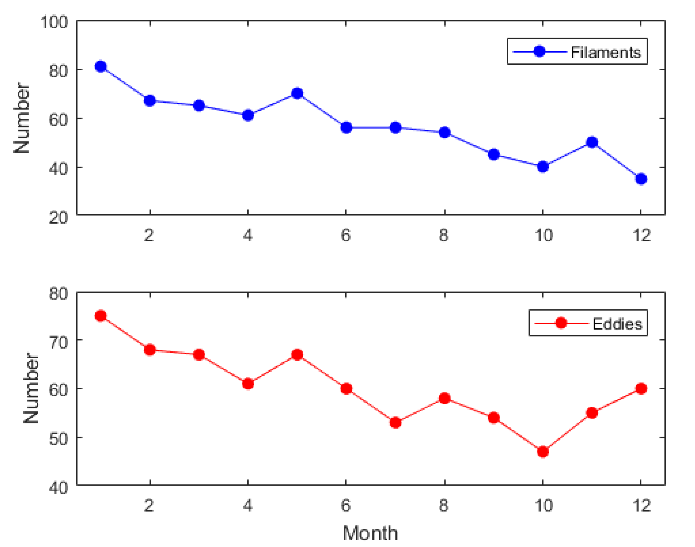
. The overall average of the occurrence probability (the number of days when a filament is present divided by the total number of days) was $54.6\%$, while the overall average filament length was about 200 km and ranged from 40 km to 716 km. In addition, the interannual variability can also be seen in both occurrence probability and filament length. The number of filaments and occurrence probability were highest in 2012 and the lowest in 2006. The number of filaments occurred in spring (MAM), summer (JJA), autumn (SON) and winter (DJF) are 196, 166, 135 and 183, respectively. Monthly count of warm filaments is shown in Figure 5. It is interesting to see a similar trend of mesoscale eddies (counted within the region from ${120}^{\circ }\mathrm{E}$ to ${125}^{\circ }\mathrm{E}$, ${16}^{\circ }\mathrm{N}$ to ${26}^{\circ }\mathrm{N}$ with the mesoscale eddy atlas), which indicates a linkage between warm filaments and mesoscale eddies.

To see the relationship between warm filaments and mesoscale eddies, we first classified warm filaments into four types: filament formation associated with the Kuroshio interacting with (A) an anti-cyclonic eddy, (C) a cyclonic eddy, (D) a dipole pair of opposite eddies and (N) none of the above cases. The statistics between eddy type and resulting filaments are summarized in

Table 2. Statistics of the identified warm filament types.

Type	A	C	D	N
Num.	396	106	68	110
Ratio	$58\%$	$16\%$	$10\%$	$16\%$

. In total 396 filaments arise from the interaction with an anticyclonic eddy (A), which accounts for $58\%$ of the filaments. A further $16\%$ of the filaments arise from interaction with a cyclonic eddy (C). In case A(C), the filament typically occurs near the north (south) of the anticyclonic (cyclonic) eddy, as were be illustrated later. Roughly $10\%$ of the filaments (D) are observed to be located between a dipole pair of cyclonic and anticyclonic eddies. The remaining 16% of the observed filaments do not correspond to any of the three above cases.

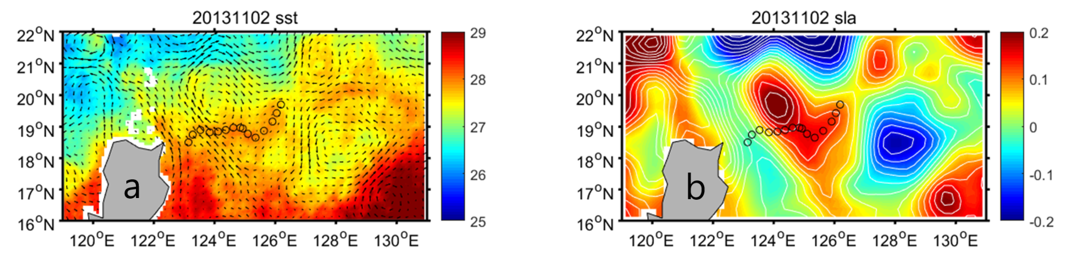
The strong coincidence of warm filaments and the proximity of eddies suggests that the filaments are probably pulled out of the Kuroshio by eddies. This is readily apparent in Figure 1 and Figure 2, where a warm filament indeed appears to be drawn out by the current interaction with an eddy. Figure 6 plots the average latitude of each warm filament against the latitude of the associated eddy center. In the anticyclonic case, most of the data points are under the line of slope 1, which means the warm filaments are located more northward than the corresponding eddies, because an anticyclonic eddy usually strips off a filament on its northern side. Conversely, warm filaments are always stripped off from the southern side of a cyclonic eddy. Thus, we can expect the speed on the northwestern (southwestern) flank of an anticyclonic (cyclonic) eddy to have the greatest impact on the strength of warm filaments. We denote the latitudes of filament and eddy as $L_f,L_e$, respectively, and define $L_r=L_f-L_e$ as the average distance between the eddy center and filament. From the data we found $L_r={0.57}^{\circ }$ ($L_r=-{0.51}^{\circ }$) for the anticyclonic (cyclonic) case, which is slightly smaller than the corresponding eddy radius. 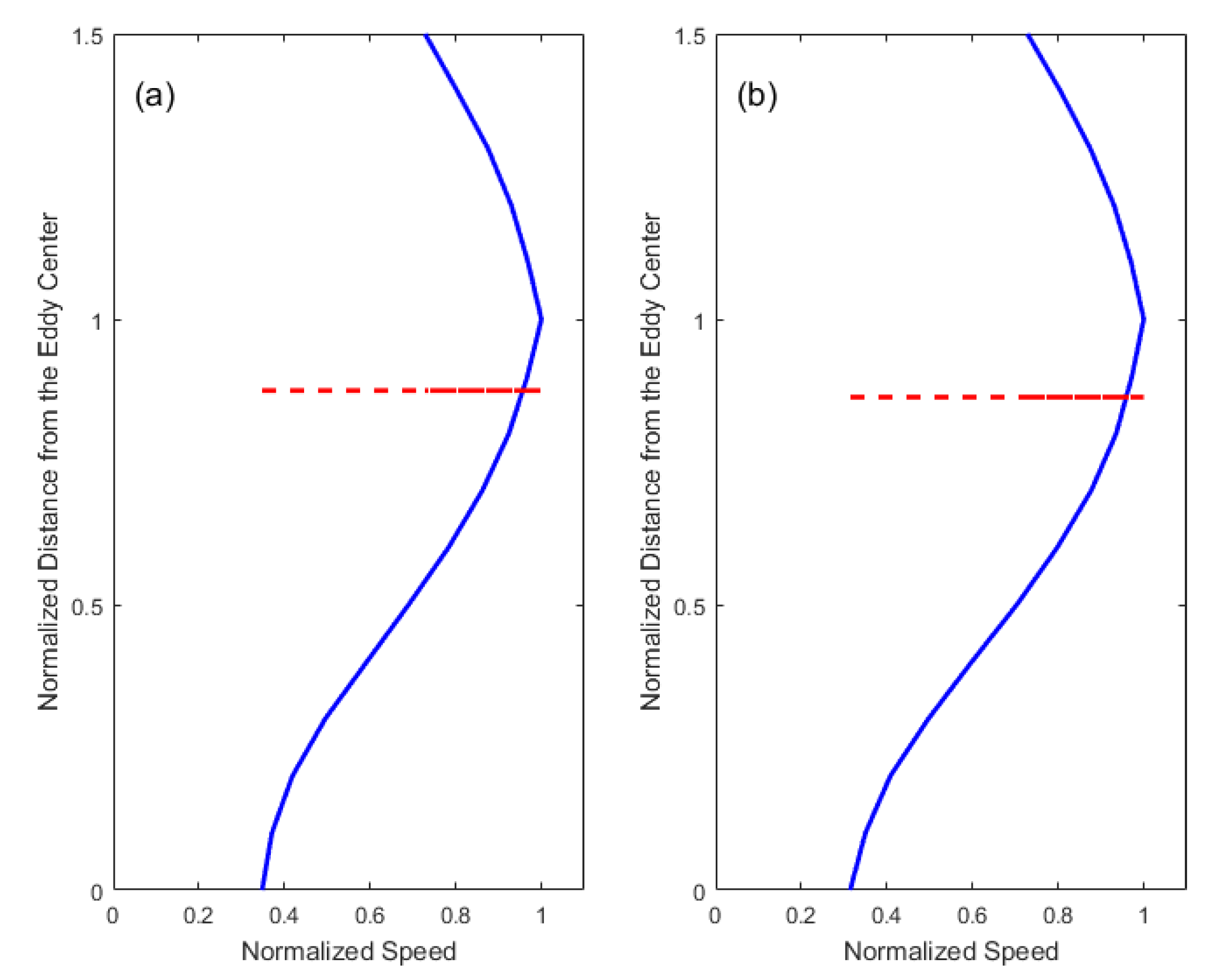To examine where the filament is located relative to the eddy center, Figure 7 shows a radial profile of eddy current speed from the eddy center towards the nearest point on the filament. The speed and distance are normalized by the magnitude and radial distance of the location of maximum-speed of an eddy, respectively. It can be seen that the warm filaments usually occur at around 0.88 (0.86) of the eddy radius (defined as the radial distance of the location of maximum-speed of an eddy) north (south) of the eddy center for the anticyclonic (cyclonic) eddy case.

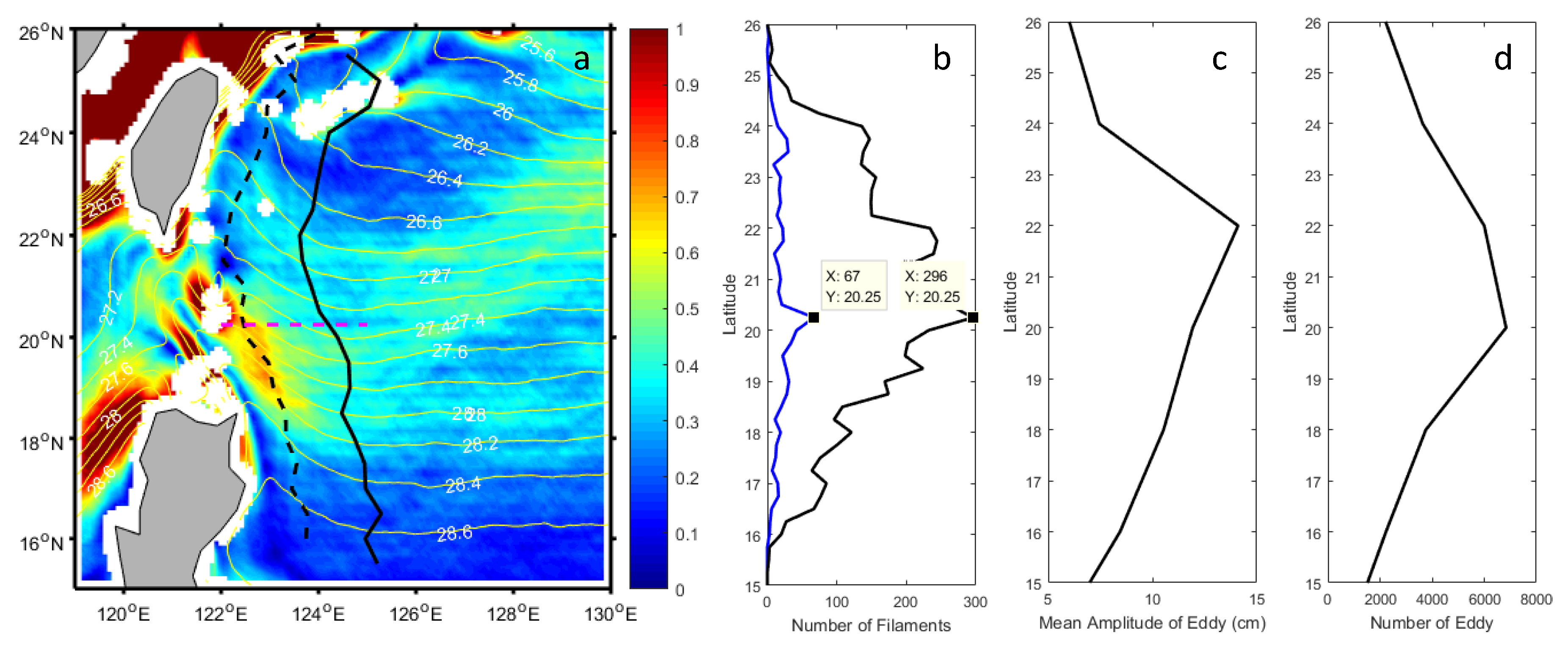
To further see the spatial relationship between warm filaments and eddies, the origination points of all warm filaments are shown in Figure 8b and there is a peak in the number of filaments at around 20° N. It is interesting to note that eddies are also most frequent and strongest at this latitude (Figure 8c,d), lending further evidence of the close relationship between warm filaments and eddies. In addition, the climatological SST gradient is also strongest in the latitude band between 19° N to 21° N (Figure 8a), which suggests that the SST gradient may also play a role in the high occurrence probability of filaments at this latitude.

4. Discussion: Dynamic Linkage between Warm Filaments, the Kuroshio Front and the Associated Eddies

The above observations suggest that warm filaments are primarily influenced by two factors: the SST gradient across the Kuroshio and the presence of mesoscale eddies (Figure 8). To quantify the relationships between them, the linkages between filament length/strength, the Kuroshio and mesoscale eddies were statistically analyzed.

We define the filament length as the curve length between the filament origin and terminus. Longer filaments transport the heat further into the ocean interior. It is interesting to note that the eddy intensity (speed) is the main factor affecting the filament length. Figure 9a gives the distribution of mean speed along the filament and the corresponding filament length with the linear least squares fit ($r^2=0.75$) superimposed. A group average has been taken for data locating in each of the equidistant intervals along x-axis to generate the scatter plots in Figure 9. As the mean speed along the filament increases, the length of the filament also increases. As the mean speed along the filament is effectively part of an eddy, the close relation between eddy intensity and filament length is to be expected; a stronger eddy will make a longer filament (Figure 9b). Here, the correlation coefficient reaches 0.83.

Surprisingly, the SST gradient of the Kuroshio was found to be largely irrelevant to the filament length (figure not shown), but we find it sometimes significantly affects the filament strength (Figure 9c). As an indicator of the filament strength, the mean cross-filament SST gradient along the filament axis was observed to be positively correlated ($r^2=0.79$) with the local SST gradient of the Kuroshio. We conclude that the Kuroshio provides an imprint of the SST gradient that determines the filament strength, but heat advection processes, driven by mesoscale eddies, is the most important for determining filament length.

To see the dependencies of warm filaments on eddy strength and the Kuroshio’s lateral SST gradient, two groups of experiments were carried out with a simple model. In the ideal model, the equation for the mixed layer temperature tendency reads

$$\frac{\partial T}{\partial t}=-\left(u_g\frac{\partial T}{\partial x}+v_g\frac{\partial T}{\partial y}\right)$$

(1)

where T is the SST or the mixed layer temperature and $u_g$, $v_g$ are zonal and meridional components of the geostrophic current respectively [26]. In ideal experiments, we adopted the Taylor vortex model [27] whose circumferential velocity is specified as,

$$\begin{array}{cc}\hfill \left|V\right(r\left)\right|& =A_{0}r\exp (-\frac{r^2}{2A_1^2}),\hfill \end{array}$$

where r is the radial distance from the eddy center $(x_0,y_0)$. $A_1$ scales the radius of the eddy so that the circumferential velocity reaches a maximum at $r=A_1$. $A_0$ is the strength of the eddy velocity. The Kuroshio’s streamwise velocity is described by an idealized Gaussian profile:

$$\begin{array}{cc}\hfill v_c& =C_0\exp (-C_1^2{(x-x_c)}^2),\hfill \end{array}$$

where $x_c$ denotes the longitude of the current’s central axis. $C_0$ determines the maximum velocity on the current and $C_1$ is the inverse of the cross-stream decay scale. According to the observed and simulated SST on the Kuroshio (e.g., Figure 1 in [28]), the initial temperature distribution is set to be:

$$\begin{array}{cc}\hfill T& =T_0+T_1\exp (-C_1^2{(x-x_c)}^2),\hfill \end{array}$$

where $T_0$ sets the uniform background temperature and $T_1$ controls the maximum temperature difference. The total velocity field and the initial temperature distribution of the base case ($A_0=2.0$, $C_1^2=0.4$) are exhibited in Figure 10. We adjusted $A_0$ to simulate eddies with various circumferential velocities and change $C_1$ to control the SST gradient across the current. The remaining parameters are fixed among all experiments as $x_c=120,x_0=122.5,y_0=21,A_1=0.45,C_0=0.8,T_0=27,T_1=1$.

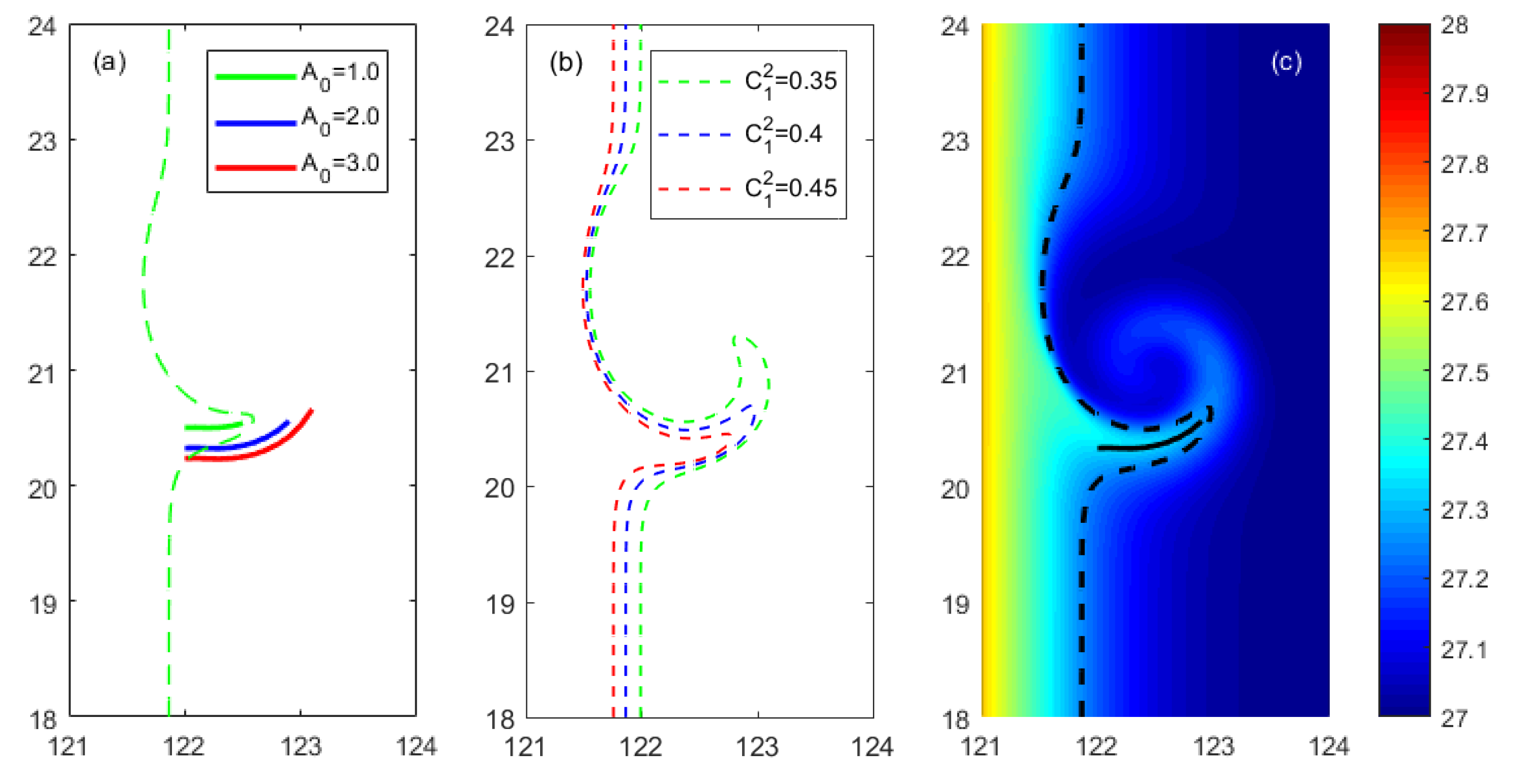
In the first group of experiments, the maximum tangential velocity of the eddy is varied by changing $A_0$ with other parameters remaining fixed. As expected, stronger eddies induce longer filaments (Figure 11a), which is consistent with the observations (Figure 9b). The filament length extends ${0.6}^{\circ }$ further in longitude as the maximum tangential eddy velocity increases from 0.3 $\mathrm{m}{\mathrm{s}}^{-1}$ to 0.8 $\mathrm{m}{\mathrm{s}}^{-1}$. Notice that stronger eddies (larger tangential velocity) also have larger advective velocity in Equation (1), which is consistent with the observations and the explanation for the features shown in Figure 9a. In the second group of experiments, the Kuroshio’s lateral SST gradient is varied, while the eddy strength remains fixed. The results are compared in Figure 11b, where we plot the 27.25 °C isotherm to display the warm filament in each trial. It can be clearly seen that stronger SST gradient (larger $C_1$) leads to a stronger filament with a narrower warm tongue (strong cross-filament SST gradient), which also agrees with the observational results shown in Figure 9c.

In brief, the linkage among the warm filaments, the associated mesoscale eddies and the Kuroshio front are manifested by the temperature equation (Equation (1)) in the mixed layer model. The advective velocity and temperature gradient combine to determine the temperature tendency. When an eddy approaches the Kuroshio, where a high temperature gradient exists, a warm filament forms and is stripped out along the eddy’s edge in a direction determined by the tangential flow of the eddy where the eddy interacts with the Kuroshio. During this process, the strong lateral temperature gradient of the Kuroshio may induce a large cross-filament temperature gradient during the advection process, which further contributes to the filament strength. In addition, a stronger eddy also tends to advect the filament further out along its edge.

5. Summary and Concluding Remarks

Spatial distributions of warm filaments near the Kuroshio were presented and analyzed for a suite of satellite observations. These filaments can extend several hundreds of kilometers out from the Kuroshio. Filaments are observed over nearly 1/3 of the year on average. The maximum mean speed along a filament can reach 0.78 $\mathrm{m}{\mathrm{s}}^{-1}$, with the average being around 0.35 $\mathrm{m}{\mathrm{s}}^{-1}$. These relatively large velocities combined with the strong SST gradients imposed by the Kuroshio mean that these filaments may play important roles in heat and material exchange near the Kuroshio.

The warm filaments are also very likely to be observed near the Luzon Strait. This can probably be attributed to the instability of Kuroshio there, reflected by the pronounced meandering of the current’s path. The formation of a warm filament is found to be highly correlated with the interaction between the Kuroshio and westward propagating mesoscale eddies (especially anticyclonic eddies). It is interesting to see anticyclonic eddies can pull out much more warm filaments than cyclonic eddies when they meet the Kuroshio. As indicated by Figure 4 in [28], a possible explanation is that an anticyclonic eddy tends to advect warm water from south to north and further pulls warm water out from the Kuroshio, whereas a cyclonic eddy conveys cold water in the opposite direction and may suppress the formation of warm filaments.

For eddy induced filaments, the direction a filament that is drawn out of the Kuroshio is dictated by the type of the eddy. The strength of the eddy contributes to the advection velocity along the filament, which further affects the overall length of the filament. The strength of a filament, proportional to the cross-filament averaged temperature gradient, is related to SST gradient imprinted by the Kuroshio at the latitude where it interacts with the eddy. The above mechanisms can be explained by the mixed layer temperature tendency equation. The present results indicate that the warm filaments not only play influential roles in the heat and material transport, but also provide insights into the current-eddy interactions.

We also notice some other interesting aspects for warm filaments identified from the SST maps. For example, an “N-case” warm filament is shown in Figure 12. This filament has one end on the Kuroshio, but falls on the southern flank of an anticyclonic eddy. This is the opposite to the flow direction typical of an “A-case” interaction and it suggests that the filament did not originate from the Kuroshio, but from an adjacent cyclonic eddy. The SST evolution shows that the cyclonic eddy grabs warm water located to the south, forming a warmer edge, which is transported to the anticyclonic eddy through eddy–eddy interaction. Therefore, in a train of mesoscale eddies, warmer water can be advected along the eddies’ flanks and can be transported several hundred kilometers. We have observed some long warm filaments (more than 800 km) in the Western Pacific Ocean. This conveyor belt through a train of mesoscale eddies may provide a mechanism to transport heat from the equatorial currents into the interior of the ocean.

References

1. Flament, P.; Armi, L.; Washburn, L. The evolving structure of an upwelling filament. J. Geophys. Res. Ocean. 1985, 90, 11765–11778. [Google Scholar] [CrossRef] [Green Version]
2. Ribbe, J.; Brieva, D. A western boundary current eddy characterisation study. Estuar. Coast. Shelf Sci. 2016, 183, 203–212. [Google Scholar] [CrossRef] [Green Version]
3. Ribbe, J.; Toaspern, L.; Wolff, J.O.; Ismail, M.F.A. Frontal eddies along a western boundary current. Cont. Shelf Res. 2018, 165, 51–59. [Google Scholar] [CrossRef]
4. Mooers, C.N.; Robinson, A.R. Turbulent jets and eddies in the California Current and inferred cross-shore transports. Science 1984, 223, 51–53. [Google Scholar] [CrossRef]
5. Strub, P.T.; Kosro, P.M.; Huyer, A. The nature of the cold filaments in the California Current System. J. Geophys. Res. Ocean. 1991, 96, 14743–14768. [Google Scholar] [CrossRef]
6. Barton, E.; Inall, M.; Sherwin, T.; Torres, R. Vertical structure, turbulent mixing and fluxes during Lagrangian observations of an upwelling filament system off Northwest Iberia. Prog. Oceanogr. 2001, 51, 249–267. [Google Scholar] [CrossRef] [Green Version]
7. Peliz, Á.; Santos, A.M.P.; Oliveira, P.B.; Dubert, J. Extreme cross-shelf transport induced by eddy interactions southwest of Iberia in winter 2001. Geophys. Res. Lett. 2004, 31. [Google Scholar] [CrossRef]
8. Meunier, T.; Barton, E.D.; Barreiro, B.; Torres, R. Upwelling filaments off Cap Blanc: Interaction of the NW African upwelling current and the Cape Verde frontal zone eddy field? J. Geophys. Res. Ocean. 2012, 117. [Google Scholar] [CrossRef] [Green Version]
9. Lutjeharms, J.; Shillington, F.; Rae, C.D. Observations of extreme upwelling filaments in the Southeast Atlantic Ocean. Science 1991, 253, 774–776. [Google Scholar] [CrossRef] [PubMed]
10. Li, J.; Wang, G.; Zhai, X. Observed cold filaments associated with mesoscale eddies in the South China Sea. J. Geophys. Res. Ocean. 2017, 122, 762–770. [Google Scholar] [CrossRef]
11. Xie, S.P.; Xie, Q.; Wang, D.; Liu, W.T. Summer upwelling in the South China Sea and its role in regional climate variations. J. Geophys. Res. Ocean. 2003, 108. [Google Scholar] [CrossRef] [Green Version]
12. Xie, S.P.; Chang, C.H.; Xie, Q.; Wang, D. Intraseasonal variability in the summer South China Sea: Wind jet, cold filament, and recirculations. J. Geophys. Res. Ocean. 2007, 112. [Google Scholar] [CrossRef]
13. Sullivan, P.; McWilliams, J. Frontogenesis and frontal arrest of a dense filament in the oceanic surface boundary layer. J. Fluid Mech. 2018, 837, 341–380. [Google Scholar] [CrossRef]
14. Washburn, L.; Swenson, M.S.; Largier, J.L.; Kosro, P.M.; Ramp, S.R. Cross-Shelf Sediment Transport by an Anticyclonic Eddy Off Northern California. Science 1993, 261, 1560–1564. [Google Scholar] [CrossRef] [PubMed] [Green Version]
15. Yasuda, I.; Okuda, K.; Hirai, M. Evolution of a Kuroshio warm-core ring -Variability of the hydrographic structure. Deep. Sea Res. 1992, Part A, S131–S161. [Google Scholar] [CrossRef]
16. Xie, S.P.; Liu, W.T.; Liu, Q.; Nonaka, M. Far-reaching effects of the Hawaiian Islands on the Pacific ocean-atmosphere system. Science 2001, 292, 2057–2060. [Google Scholar] [CrossRef] [Green Version]
17. Xie, S.P. Satellite observations of cool ocean–atmosphere interaction. Bull. Am. Meteorol. Soc. 2004, 85, 195–208. [Google Scholar] [CrossRef] [Green Version]
18. Kawai, Y.; Nishikawa, H.; Oka, E. In Situ Evidence of Low-Level Atmospheric Responses to the Oyashio Front in Early Spring. J. Meteorol. Soc. Jpn. 2019, 97, 423–438. [Google Scholar] [CrossRef]
19. Kawai, H.; Saitoh, S. Secondary fronts, warm tongues and warm streamers of the Kuroshio Extension system. Deep. Sea Res. Part Oceanogr. Res. Pap. 1986, 33, 1487–1507. [Google Scholar] [CrossRef]
20. Ichikawa, H.; Chaen, M. Seasonal variation of heat and freshwater transports by the Kuroshio in the East China Sea. J. Mar. Syst. 2000, 24, 119–129. [Google Scholar] [CrossRef]
21. Chen, S. The Kuroshio Extension Front from satellite sea surface temperature measurements. J. Oceanogr. 2008, 64, 891–897. [Google Scholar] [CrossRef]
22. Guo, B.; Xiu, S.; Ishii, H.; Nakamura, Y. Kuroshio warm filament and the source of the warm water of the Tsushima Current. Acta Oceanol. Sin. 1991, 10, 325–340. [Google Scholar]
23. Chelton, D.B.; Schlax, M.G.; Samelson, R.M. Global observations of nonlinear mesoscale eddies. Prog. Oceanogr. 2011, 91, 167–216. [Google Scholar] [CrossRef]
24. Holyer, R.J.; Peckinpaugh, S.H. Edge detection applied to satellite imagery of the oceans. IEEE Trans. Geosci. Remote Sens. 1989, 27, 46–56. [Google Scholar] [CrossRef] [Green Version]
25. Wang, G.; Su, J.; Chu, P.C. Mesoscale eddies in the South China Sea observed with altimeter data. Geophys. Res. Lett. 2003, 30. [Google Scholar] [CrossRef] [Green Version]
26. Qu, T. Role of ocean dynamics in determining the mean seasonal cycle of the South China Sea surface temperature. J. Geophys. Res. Ocean. 2001, 106, 6943–6955. [Google Scholar] [CrossRef]
27. Wu, J.Z.; Ma, H.Y.; Zhou, M.D. Vorticity and Vortex Dynamics; Springer Science & Business Media: Berlin/Heidelberg, Germany, 2007. [Google Scholar]
28. Sun, R.; Wang, G.; Chen, C. The Kuroshio bifurcation associated with islands at the Luzon Strait. Geophys. Res. Lett. 2016, 43, 5768–5774. [Google Scholar] [CrossRef] [Green Version]
Figure 1. Snapshot of (a) SST (color, °C) and geostrophic velocity (vectors); (b) sea level anomalies (SLA) (color, in m) and absolute dynamic topography (ADT) contours on 2 March 2010. Warm filaments are marked by small circles in the lower right quadrant of the frame accompanied by an anticyclonic eddy.
Remotesensing 12 03090 g001
Figure 2. Snapshot of (a) SST (color, C ) and geostrophic velocity (vectors); (b) SLA (color, in m) and ADT contours on 15 February 2006. Warm filaments are marked by small circles near the center of the frame accompanied by a cyclonic eddy.
Remotesensing 12 03090 g002
Figure 3. Snapshot of (a) SST (color, C ) and geostrophic velocity (vectors); (b) SLA (color, in m) and ADT contours on 01 April 2009. Warm filaments are marked by small circles near the center of the frame accompanied by a dipole pair of opposite eddies.
Remotesensing 12 03090 g003
Figure 4. (a) Snapshot of all the detected warm filaments. (b) Warm filaments in each 0.5 × 0.5 box.
Remotesensing 12 03090 g004
Figure 5. Numbers of warm filaments (upper panel) and mesoscale eddies (lower panel) that occurred in each month. The count of eddies is based on Chelton’s eddy atlas.
Remotesensing 12 03090 g005
Figure 6. Eddy center position versus warm filament latitude for (a) the anticyclonic eddy case and (b) the cyclonic eddy case. The dashed line is the auxiliary line with slope of 1.
Remotesensing 12 03090 g006
Figure 7. The radial mean profile of current speed from the eddy center towards filament. The speed and the distance are normalized by the magnitude and radial distance at the location of maximum-speed of an eddy respectively: (a) anticyclonic case; (b) cyclonic case. Red dashed line marks the mean position where filaments occur.
Remotesensing 12 03090 g007
Figure 8. (a) SST ( C , yellow contours) and SST gradient ( C / longitude, color shading) for the SST climatology. The dashed (solid) black line is the average occurrence (end) points of warm filaments for each 0.25 meridional grid. The dashed magenta line marks latitude 20.25° N. (b) Distribution of the number of warm filaments that appear (black line) and occurrence probability (blue line) in each 0.25° latitude bin. (c) Distributions of mean eddy amplitudes (cm) for each 2° latitude bin based on the mesoscale eddy atlas produced by SSALTO/DUACS and distributed by AVISO+ (https://www.aviso.altimetry.fr/). (d) Distributions of the number of eddies for each 2° latitude bin.
Remotesensing 12 03090 g008
Figure 9. Scatterplots of (a) mean speed along the filament versus length of filament, (b) absolute value of SLA at eddy center versus length of filament and (c) lateral SST gradient of the Kuroshio versus SST gradient across the filament, each with best fit linear regression.
Remotesensing 12 03090 g009
Figure 10. (a) Velocity field (vectors) for the ideal experiment. Color: speed ( m s 1 ). (b) Initial temperature distribution ( C ).
Remotesensing 12 03090 g010
Figure 11. Filaments for (a) various eddy tangential velocities, (b) various lateral SST gradients across the Kuroshio. Dashed lines: isotherms. Solid lines: detected warm filaments. (c) The temperature field for the baseline case. The contour and central curve illustrate the width and length of the warm filament, respectively.
Remotesensing 12 03090 g011
Figure 12. Snapshot of (a) SST (color, °C) and geostrophic velocity (vectors); (b) SLA (color, in m) and ADT contours on 2 November 2013.
Remotesensing 12 03090 g012