GNSS/INS-Equipped Buoys for Altimetry Validation: Lessons Learnt and New Directions from the Bass Strait Validation Facility

Abstract

Global Navigation Satellite System (GNSS)-equipped buoys have a fundamental role in the validation of satellite altimetry. Requirements to validate next generation altimeter missions are demanding and call for a greater understanding of the systematic errors associated with the buoy approach. In this paper, we assess the present-day buoy precision using archived data from the Bass Strait validation facility. We explore potential improvements in buoy precision by addressing two previously ignored issues: changes to buoyancy as a function of external forcing, and biases induced by platform dynamics. Our results indicate the precision of our buoy against in situ mooring data is ~15 mm, with a ~8.5 mm systematic noise floor. Investigation into the tether tension effect on buoyancy showed strong correlation between currents, wind stress and buoy-against-mooring residuals. Our initial empirical correction achieved a reduction of 5 mm in the standard deviation of the residuals, with a 51% decrease in variance over low frequency bands. Corrections associated with platform orientation from an Inertial Navigation System (INS) unit showed centimetre-level magnitude and are expected to be higher under rougher sea states. Finally, we conclude with further possible improvements to meet validation requirements for the future Surface Water Ocean Topography (SWOT) mission.

1. Introduction

With a record length now approaching 30 years, satellite altimetry is an established observational tool central to the understanding of Earth’s ocean circulation and its response to a warming climate [1,2,3]. The societal importance of the altimeter sea level climate record underscores the requirement for a sustained and rigorous calibration and validation (cal/val) of the observational dataset. Unsurprisingly, in situ validation continues to form a significant component of mission design, assisting mission teams to diagnose problems and ensure confidence in the resultant mission geophysical data record (GDR).

Improvements in the altimeter measurement systems in the precision-era of altimetry commencing with TOPEX/Poseidon (1992) have enabled the improved understanding of ocean circulation and investigation into the spatiotemporal evolution of large-scale ocean processes [4,5,6]. Altimeters have progressed from Low Resolution Mode (LRM) with a pulse-limited circular footprint (e.g., Jason-series missions) to Synthetic-Aperture Radar (SAR) with a more focused Doppler-partitioned rectangular footprint (e.g., Sentinel-3A and Sentinal-3B). This heritage of radar design has seen along-track resolution evolve from ~5–10 km (LRM) to ~300 m (SAR). The community is now on the threshold of the first swath-based interferometric approach to sea surface height (SSH) determination with the launch of the SWOT mission planned for early 2022 [7]. The ambitious SWOT mission will provide the first measurements over a ~140 km wide swath at 500 m–2 km spatial resolution [8]. These advances in technology and associated science goals have brought with them increasingly demanding cal/val requirements [9], notably the “1 cm challenge” as identified upon the launch of OSTM/Jason-2 [10].

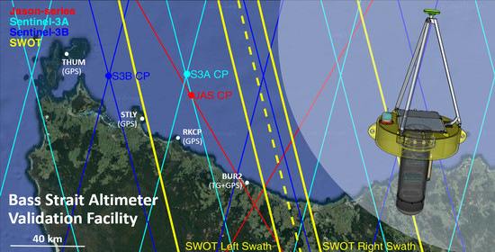
The Bass Strait altimeter validation facility (Figure 1) has made a long-standing contribution to multiple missions providing altimeter bias estimates since the launch of TOPEX/Poseidon. The facility presently contributes cycle-by-cycle estimates of absolute bias to the Ocean Surface Topography Science Team (OSTST) for the Jason-series missions, and to the Sentinel-3 Validation Team (S3VT) for the Sentinel-3A and Sentinel-3B missions. The site and its geometric validation approach to classical nadir altimetry is well understood [11,12,13,14,15,16]. Central to this validation methodology and the focus of this paper is the use of GNSS-equipped buoys capable of determining absolute SSH in the same reference frame as the altimeters.

Here, given the challenge presented by the SWOT mission, this paper returns to data already collected at the Bass Strait facility to quantify the precision currently achieved by GNSS-equipped buoys (in this paper we refer generically to GNSS data throughout; yet given our use of archived data that tracked a single constellation, we process data only from the Global Positioning System (GPS)). We then seek to further identify and investigate two key systematic error sources that remain a challenge for GNSS derived water level measurement. First, the variable buoyancy position of the buoy as a function of external forcing (current and waves); and second, the effect of dynamic changes in antenna position/orientation as a function of sea state. With the assistance of co-located moored oceanographic instruments and operational atmospheric model output, we use existing GNSS-buoy data to develop an empirical model to quantify the buoyancy variation as a function of current and wind stress. We then present initial results that couple inertial navigation system (INS) data with GNSS in an updated approach to relative GNSS processing. We conclude with perspectives from the Bass Strait facility in the context of the challenges associated with geometric/geodetic validation of the SWOT mission.

2. Background

GNSS-equipped floating platforms have long been used to observe SSH for a range of applications. Early efforts were focused on establishing the technique and preparing for altimetry validation (e.g., [17,18,19]). Bonnefond et al. [20] installed two GNSS receivers on a catamaran to observe the marine geoid which was later used for validation of Jason-1 at the Corsica site operated by the Centre National D’Etudes Spatiales (CNES, the French Space Agency). The positional variation between two closely placed GNSS antennae on the catamaran was 12 mm, which was presented as the zero-baseline systematic noise of the GNSS system. Further, their work had a 5 mm Root Mean Square (RMS) when referenced against the tide gauge (TG) located 100 m from the buoy. The small RMS arguably benefitted from near shore calm sea states and short baseline GNSS processing. Watson et al. [15] used a single buoy setup deployed in the open ocean directly above an array of moored oceanographic sensors (pressure, temperature and salinity to yield dynamic height). Their study obtained a larger RMS between the buoy and in situ mooring data of ~21 mm, yet they suggested the dominant driver of this variability was thought to originate from the buoy.

Later, Fund et al. [21] assessed the kinematic Precise Point Positioning (PPP) processing strategy using a similar buoy configuration. Their study showed some significant differences between results using PPP and relative positioning, yielding an RMS against a close-by radar tide gauge sampling at 1-min interval of ~49 mm for PPP compared with ~6 mm for the relative solution. The driver of the large noise in PPP was thought to originate from poor tropospheric estimates that eventually propagated into position parameters. More recently, case studies investigated the use of GNSS onboard wave-gliders [22,23] with a PPP processing strategy and achieved a precision of ~20 mm. Other groups such as Haines et al. [24] have also shown promising results using the PPP approach with a series of recent buoy experiments nearby the Harvest platform.

Regardless of the design of the floating platform (spar buoy, wave rider, glider or boat-like vessel) or the processing strategy (relative or PPP), all studies have confirmed that GNSS-equipped floating platforms can yield centimetre-level SSH measurements, thereby providing an effective tool for geometric altimeter validation. However, studies to date have not yet quantified nor shown improvement relating to two key issues faced with positioning using GNSS in the marine domain.

First, buoys anchored via a tether will likely have a time variable mean buoyancy position as a function of the force induced by surface currents, swell and wind waves (see for example the early work by Haines et al. [24]). As the tension correlates with the combined force of the wind and currents, a quasi-periodic signal that is potentially aliased with tidal elevation is likely to result in affecting the derived quantities of interest. Second, unlike land based GNSS deployments, the attitude of the platform is ever-changing with the dynamic water surface. This violates the basic assumption that the antenna is pointed to zenith and fixed in a known orientation. While smoothing of high-frequency kinematic output will reduce the magnitude of these effects, it cannot eliminate them completely since the buoy seldom returns to its “original” orientation over a short period of time. As a result, biases resulting from unmodelled changes in orientation at high frequencies will be present at some level in the SSH record. Inertial sensors have the ability to observe this motion—they have long been used in ocean-going wave-rider style buoys focused on the determination of wave characteristics [25,26,27] rather than precise sea-surface height. Coupling of GNSS/INS and its impact on positional results is much needed and worthy of further investigation.

3. Data

3.1. GNSS/INS Data

To address the precision obtainable from GNSS-equipped buoys, we return to data previously collected for routine operations at the Jason-series comparison point (JAS CP, Figure 1) at the Bass Strait validation facility. A total of ~84 days of 1 Hz GPS data from 27 deployments between 2012 to 2018 are investigated. The dataset enables an inter-comparison against co-located mooring data to determine the overarching SSH precision of the UTas/IMOS Mk-IV buoy system. Among the full-length dataset, for the purpose of redundancy, episodic dual-buoy deployments consist of deploying two identical GNSS buoys (both of the Mk-IV design henceforth referred to as Buoy 3 and Buoy 4) within 20–40 m of each other for a duration of ~48 h. 15 dual-buoy deployments were completed, a total of ~27 days of 1 Hz data. This subset enables the determination of a near-zero baseline benchmark for assessing GNSS systematic noise in the determination of differential SSH (δSSH) using the same buoy system. The deployment location is ~29 and ~25 km from GNSS reference stations located at Stanley (STLY) and Rocky Cape (RKCP) on the coastline of North West Tasmania respectively (Figure 1). We note the mean significant wave height (SWH) of this dataset is just over 1 m reflecting the calm-moderate conditions typically chosen for deployments at this facility.

In addition to the historical dataset, we also use a newly collected dataset with a micro-electromechanical system (MEMS)-based INS unit [28] (see Table S1 for specifications) installed on the Mk-IV Buoy 4 platform. This deployment took place in November 2019 where GPS data and INS data were collected at 2 Hz and 100 Hz, respectively, over a duration of 48 h. These data facilitate an early investigation of the effect of attitude variation on SSH time series.

3.2. Mooring and Oceanographic Data

Routine altimeter bias computations at the Bass Strait facility involves the use of an in situ sea level record derived from an array of moored oceanographic instrumentation co-located at the comparison point. The mooring includes an SBE26+ bottom mounted pressure gauge (at ~51 m depth) with temperature and salinity sensors (Seabird SBE37) located throughout the water column. The bottom pressure is integrated through the water column with density estimated from the temperature and salinity observations. The atmospheric pressure is removed using measurements from the Burnie tide gauge location, corrected for the differential atmospheric pressure between Burnie and the mooring site estimated using the hindcast operational atmospheric model known as the Australian Community Climate and Earth-System Simulator (ACCESS). These datasets provide a precise sea level time series (mooring SSH) on an arbitrary datum at 5-min sampling (see [15] for further detail regarding the derivation of this time series).

To investigate the potential effect of external forcing (i.e., tether tension) on buoyancy position, we focus on a key individual deployment in August 2015. In addition to the in situ sea level time series derived from the mooring array, we utilise u (Eastward) and v (Northward) upper water column currents (20-min sampling) derived from a current-meter (Nortek Aquadopp^®) mounted on the oceanographic mooring line at mid depth. Hourly wind stress at the comparison point location was extracted from the Australian regional model output ACCESS (August 2010 release [29]) to further assist the investigation.

4. Method

4.1. Existing GNSS Processing

All historical GNSS buoy data were processed in differential mode under a kinematic assumption using TRACK v1.30 [30]. For each buoy deployment, Buoys 3 and 4 were processed separately using RKCP as the base station and STLY as a tightly constrained ground station. One Hz dual frequency GPS data was used to form the ionospheric-free linear combination. Initial a priori values of the total Zenith Tropospheric Delay (ZTD) were input as interpolated from grids associated with the VMF1 model [31], and the wet component was then estimated with moderate constraints of ${10}^{-5} m/\sqrt{epoch}$. The satellite elevation cut-off angle was set at 10° to ensure a well-balanced and realistic estimation of the ZTD impact on observed ranges. Other processing specifics remain as the defaults in TRACK for long baselines, such as configurations for integer ambiguity resolution and cycle slip detection and repair. Deployments were segmented into 13-h arcs with adjacent sessions overlapping by 1 h to allow high frequency (1-Hz) processing. A full description of the processing configuration can be found in Table S2.

4.2. Updated GNSS/INS Processing

4.2.1. GNSS Observational Model

To further improve GNSS solutions, we updated and implemented several corrections to the observational model used in TRACK. The solid Earth tide was updated from IERS1992 to IERS2010 [32]. Ocean tide loading was introduced using the IERS2010 standard, which considers 342 constituent tides. The propagational relativistic effect [33] was also incorporated into TRACK, implemented as a satellite quality check mechanism to eliminate bad clock estimates. Furthermore, we added the newest VMF3 [34] into TRACK which implements a direct interpolation of the mapping function parameters based on the European Centre for Medium-Range Weather Forecasts (ECMWF) Re-Analysis Interim (ERA-Interim) Pressure-Level Data [35] rather than interpolation from a priori values. The ERA-Interim pressure dataset has a horizontal resolution of $1^{°}\times 1^{°}$ and 25 vertical layers. VMF3 adopts an improved parameterization to derive mapping function coefficients compared with its predecessor, VMF1 [36]. Deployments were further segmented into 7-h arcs (each overlapping by 1-h) to allow optimal double difference arc combinations.

4.2.2. INS Integration

Buoy-derived SSH is affected by the variation of platform orientation at different stages of the processing. Correction for the variation in the phase centre of the antenna and counting of phase cycles typically assumes a horizontal antenna with fixed orientation. Mismodelling of the phase centre and miscounting of the phase cycles will lead to ambiguity resolution biases which in turn increase the uncertainty of the positional output. The very last step of reducing the derived height at the antenna reference point to the sea surface will also be biased if the correct orientation is not taken into consideration. Given these three key issues, we seek to integrate the INS observed platform orientation into the processing workflow.

From an INS integration prospective, we derived the orientations of the platform from an adaptive Extended Kalman Filter (EKF) (see Text S1 [37,38,39] for further detail) using our 9 degree-of-freedom (DOF) INS unit. Then, to address the biases induced by the orientation variations in GNSS processing, we introduced three improvements into the TRACK software as detailed below.

Adaptive Phase Centre Variation (PCV) Correction

This feature maps the real-time attitude of the antenna (heavily influenced by sea-state) onto the calibrated PCV table for the buoy platform. By using roll $\left(\phi \right)$, pitch $\left(\theta \right)$ and yaw $\left(\psi \right)$ sensed by the INS unit, the elevation and azimuth can be calculated as:

$$\{\begin{array}{c}\stackrel{\rightharpoonup }{e_u^{\prime }}=R\left(\theta \right)·R\left(\phi \right)·\stackrel{\rightharpoonup }{e_u}\\ \stackrel{\rightharpoonup }{e_e^{\prime }}=R\left(\psi \right)·R\left(\theta \right)·R\left(\phi \right)·\stackrel{\rightharpoonup }{e_e}\\ \stackrel{\rightharpoonup }{e_n^{\prime }}=R\left(\psi \right)·R\left(\theta \right)·R\left(\phi \right)·\stackrel{\rightharpoonup }{e_n}\end{array}$$

(1)

$$\{\begin{array}{c}\stackrel{\rightharpoonup }{s}=\stackrel{\rightharpoonup }{P_{sat}}-\stackrel{\rightharpoonup }{P_{rec}}\\ elevation=\frac{\pi }{2}-\arccos (\frac{\stackrel{\rightharpoonup }{e_u^{\prime }}·\stackrel{\rightharpoonup }{s}}{\Vert \stackrel{\rightharpoonup }{e_u^{\prime }}\Vert \Vert \stackrel{\rightharpoonup }{s}\Vert })\\ azimuth=atan2(\frac{\stackrel{\rightharpoonup }{e_e^{\prime }}·\stackrel{\rightharpoonup }{s}}{\Vert \stackrel{\rightharpoonup }{e_e^{\prime }}\Vert },\frac{\stackrel{\rightharpoonup }{e_n^{\prime }}·\stackrel{\rightharpoonup }{s}}{\Vert \stackrel{\rightharpoonup }{e_n^{\prime }}\Vert })\end{array}$$

(2)

where $\stackrel{\rightharpoonup }{e_e^{\prime }},\stackrel{\rightharpoonup }{e_n^{\prime }}\stackrel{\rightharpoonup }{,e_u^{\prime }}$ denote unit vectors of East, North and Up in a buoy centred local tangent plane frame; R($\phi$), R($\theta$), R($\psi$) denote rotation matrices, where $\phi , \theta , \psi$ (roll, pitch and yaw respectively) are measured along the X, Y and Z axis of the INS unit; $\stackrel{\rightharpoonup }{s}$ denotes the unit vector from station towards a satellite.

Phase Wrap-Up (PWU) Correction

PWU is a result of electromagnetic nature of circularly polarised waves intrinsic to GNSS signals. As the satellite and the ground station rotates relatively, a spurious phase variation will be induced; however, the receiver is programmed to interpret this as a range variation [40]. This effect is normally cancelled out in double-differencing solutions up to medium-length baselines. However, for a rotating buoy rover station pairing with a non-rotational ground station, it is no longer cancelled and has to be considered when forming double-differencing pairs. Hence, following Equation (30) in Wu et al. [40]:

$$\delta \varphi =sign\left(\zeta \right)·\arccos (\frac{\stackrel{\rightharpoonup }{D^{\prime }}·\stackrel{\rightharpoonup }{D}}{\Vert \stackrel{\rightharpoonup }{D^{\prime }}\Vert \Vert \stackrel{\rightharpoonup }{D}\Vert })$$

(3)

where $\stackrel{\rightharpoonup }{D},\stackrel{\rightharpoonup }{D^{\prime }}$ addresses the station and satellite side of the phase wrap-up effect respectively, and $\zeta$ address the line-of-transmission from satellite to station.

We consider two parts of this correction. When the buoy platform orientation is not available, only the satellite induced phase wrap-up is calculated (we refer to this in the latter part of this paper as static phase wrap-up). We implement this as an additional part of the standard observational model in TRACK.

On the other hand, once two consecutive epochs of orientation are known for the platform, the relative rotation between two epochs is derived first, then such rotation will be accounted into $\stackrel{\rightharpoonup }{D}$ for the station induced phase wrap-up (referred to hereon as dynamic phase wrap-up). The relative rotation between two epochs is calculated by:

$$\{\begin{array}{c}\stackrel{\rightharpoonup }{k}=\stackrel{\rightharpoonup }{a}\times \stackrel{\rightharpoonup }{b}\\ c=\Vert \stackrel{\rightharpoonup }{k}\Vert ·\sin \langle \stackrel{\rightharpoonup }{a},\stackrel{\rightharpoonup }{b}\rangle \\ {[\stackrel{\rightharpoonup }{k}]}_{\times }=\left[\begin{array}{ccc}0& -k_3& k_2\\ k_3& 0& -k_1\\ -k_2& k_1& 0\end{array}\right]\end{array}$$

(4)

$$R=I+{[\stackrel{\rightharpoonup }{k}]}_{\times }+\frac{1}{1+c}·{[\stackrel{\rightharpoonup }{k}]}_{\times }^2$$

(5)

where $\stackrel{\rightharpoonup }{a}, \stackrel{\rightharpoonup }{b}$ denote unit vectors converted from corresponding orientations at each epoch; $I$ is the identity matrix and ${[\stackrel{\rightharpoonup }{k}]}_{\times }$ is the skew symmetric matrix form generated from the cross product of the two vectors defined as above; $R$ is the relative rotation matrix between two epochs of interest.

Orientation Compensated Antenna Reference Point (ARP) Correction

This term specifically addresses the ARP reduction for the buoy platform between the antenna phase centre to the nominal centre of buoyancy of the buoy platform (and thus an instantaneous SSH measurement). The calculation will be applied based on:

$$SS{H}_{buoy}=Phase Centr{e}_{Ant}-R\left(\psi \right)·R\left(\theta \right)·R\left(\phi \right)·AR{P}_{Ant}$$

(6)

where R($\phi$), R($\theta$), R($\psi$) denote rotation matrices following the same convention as defined in (1); $Phase Centr{e}_{Ant}$ is the directly measured ellipsoidal height from the buoy antenna; $AR{P}_{Ant}$ is the constant offset specific to the buoy and $SS{H}_{buoy}$ is the derived instantaneous SSH measurement compensated for orientation.

4.3. Buoy Precision Assessment and Tether Tension Modelling

4.3.1. Overarching Precision against Mooring

To assess the overarching precision of SSH measured by the buoys, an inter-comparison between buoy and mooring time series was carried out. Given the mooring time series has a relatively low temporal resolution (5-min sampling) and is insensitive to waves, a 25-min moving mean was first applied to the 1 Hz GNSS buoy solutions. 3-sigma outlier removal was applied both before and after smoothing. Using the mooring time series as reference, we interpolated the GNSS buoy solutions to the nearest mooring epochs and computed the residual difference between the two. The standard deviation of the residual from this yielded buoy precision relative to an external in situ series, hence we refer to this as the overarching buoy precision. Note we removed the constant offset that exists in this residual—that offset (derived using all available GNSS buoy solutions) was used to define the absolute datum of the mooring time series in order to facilitate cycle-by-cycle comparison with satellite altimetry.

4.3.2. Relative Precision between Buoys

To investigate the intrinsic systematic noise within the buoy system, δSSH was calculated by differencing the SSH solutions of the two buoys from existing deployments of two identical buoys separated by ~20–40 m. Theoretically, the expected δSSH value should be zero given the proximity of the deployed buoys. However, in reality, the residual is dominated by systematic and random noise contributions from both buoys. Hence, by analysing the residual, critical information can be gained in terms of the relative precision.

To reduce the impact of wind waves and other high frequency external forcing factors, a 25-min moving mean was applied after a first round of 3-sigma outlier removal for each individual buoy deployment before differencing. Another round of more rigorous sigma-based outlier removal was applied after the differencing with consideration of the degree of freedom calculated by the Auto-Correlation Function (ACF) of the time series. The ACF-based outlier removal takes temporal correlation into consideration when handling time series [41] (Chapter 2).

4.3.3. Tether Tension Modelling

In a preliminary attempt to model the tether tension effect on the buoys in use at the Bass Strait facility, a combination of surface currents and wind stress is utilized to investigate a small but significant semi-diurnal signal apparent in some of the buoy minus mooring residuals (Figure S1). Given this aligns with the dominant semi-diurnal tidal band, we undertook this investigation using the deployment from August 2015 which appears most significantly affected by this issue. To best describe the tether tension caused by currents and wind waves, the residual between the mooring and buoy was interpolated in time to the epochs defined by the current and wind stress data, respectively. Then, current and wind stress vectors were projected onto the tether, which is defined as the direction from the anchor point to the buoy. The projection was further used as the contributing forcing from the current and wind stress, respectively.

As a result, the empirical model established for our initial investigation is:

$$\{\begin{array}{c}{T}_w=\frac{v_w}{u_w}·\sqrt{v_w^2+u_w^2}\\ T_c=\frac{v_c}{u_c}·\sqrt{v_c^2+u_c^2}\\ R_M=s_w·{\left(T_w\right)}^{\frac{1}{e_w}}+s_c·{(T_c)}^{\frac{1}{e_c}}\end{array}$$

(7)

where $T_w$ and $T_c$ represents the contributing forcing from wind stress and currents with subscript $w$ and $c$ as wind stress and currents respectively; $\left(v_w, u_w\right) \mathrm{and} \left(v_c, u_c\right)$ denotes the vectors projected onto the tether direction, with $v$ as the northward component, $u$ as the eastward component; $R_M$ denotes the modelled residual induced by wind and currents; $s$ parameters denote scale factors to counterbalance the unknown scale of the input with respect to the actual force on the tether, while the $e$ parameter denotes an exponential coefficient.

A constrained local minimizer was used to solve for the above parameterisation. The standard deviation of the difference between the residual and the modelled series was used as the objective function to be minimized. A penalty function was built based on the standard deviation and mean of the difference to help the search of the optimal set of parameters.

5. Results

5.1. Benchmarking GNSS-Buoy Overarching SSH Precision

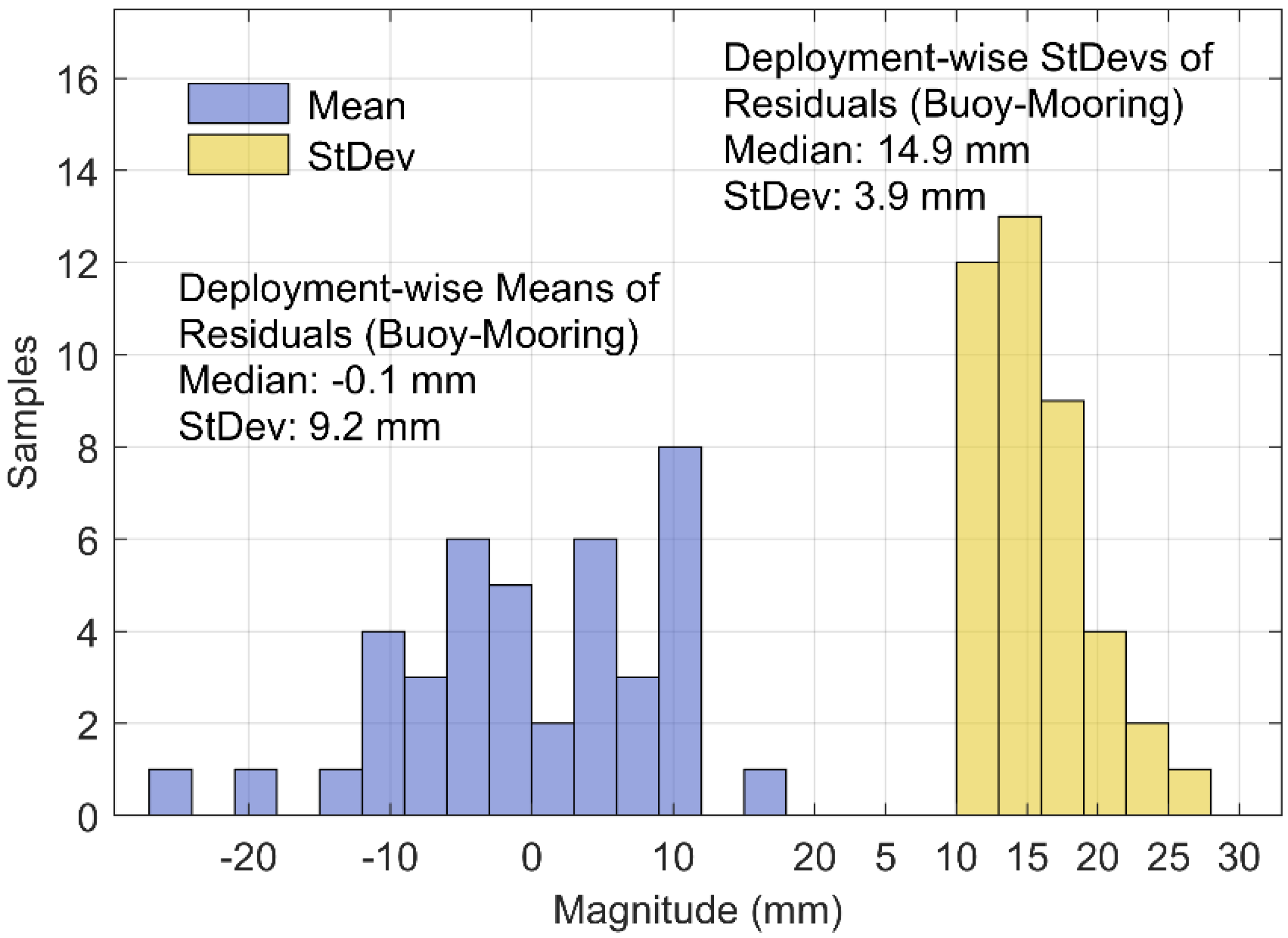
Figure 2 shows summary statistics for the historical deployments at Bass Strait between 2012 and 2018, all of which had co-located mooring data for reference. The mean and standard deviation between the mooring and buoy is computed for each deployment, and then shown as a histogram. The deployment-wise mean differences between the mooring and buoy time series appears reasonably normally distributed with a median of −0.1 mm and a standard deviation of 9.2 mm, while the buoy minus mooring residual has an average 14.9 mm standard deviation, with 3.9 mm scatter within the deviation values.

In general, a reasonable consistency is seen between the measured SSH from the buoy and mooring, with a negligible bias in the mean and a standard deviation around 15 mm for most deployments. Four deployments had mean absolute differences against the mooring above 15 mm. The contribution of potential errors in the mooring cannot be ignored here and we return to this point in the discussion. Of interest however, there are seven deployments with residuals having a standard deviation above 20 mm. This higher-than-usual variability is expressed largely as a quasi-semi-diurnal periodic signal (Figure S1) in the residual, and requires further investigation as outlined below. The August 2015 deployment used to investigate the effect of external forcing, for example, had a standard deviation of 19.5 mm and 20.4 mm respectively for each buoy deployed.

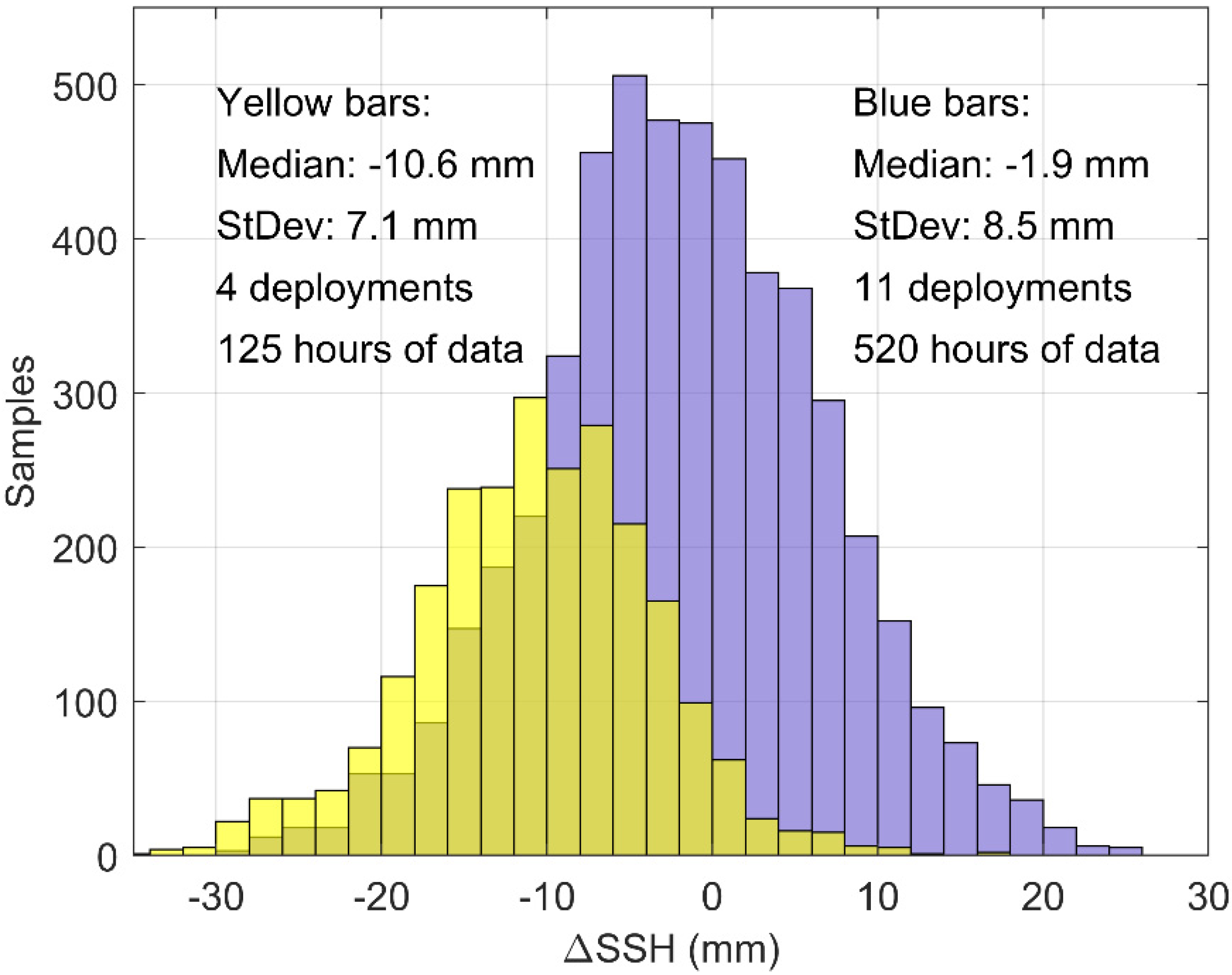
5.2. Benchmarking GNSS-Buoy Relative SSH Precision

Of all 15 deployments where we had a pair of buoys deployed in close proximity, 11 deployments with a total length of 520 h of data passed the outlier removal tests. In Figure 3, blue bars show differences between both buoys, which presents as a very well-shaped normal distribution with a median of −1.9 mm and a standard deviation of 8.5 mm.

On the other hand, yellow bars in Figure 3 show four excluded deployments with an obvious yet unknown mean bias of −10.6 mm. We are unable to attribute this bias to any change in buoy mass (i.e., buoyancy position) and suspect an undocumented change to the deployment tether. However, it is worth noting that the standard deviation is well within the range of 8.5 mm, comparable to those 11 deployments included. Hence, we consider a standard deviation of 8.5 mm as the intrinsic systematic noise within the buoy system, including issues arising from subtle differences in the construction of both buoys and processing errors.

Considering the mean buoy-mooring standard deviation of 15 mm (Section 3.1), the δSSH standard deviation of 8.5 mm suggests a significant component of the variability can be accounted for by buoy-related systematic error. There is, however, a large proportion that is not currently well understood and includes contributions from GNSS processing related issues that do not cancel as happens when forming the δSSH. Other contributions include mooring error and systematic effects on the buoy such as buoyancy changes as a function of tether tension and dynamics.

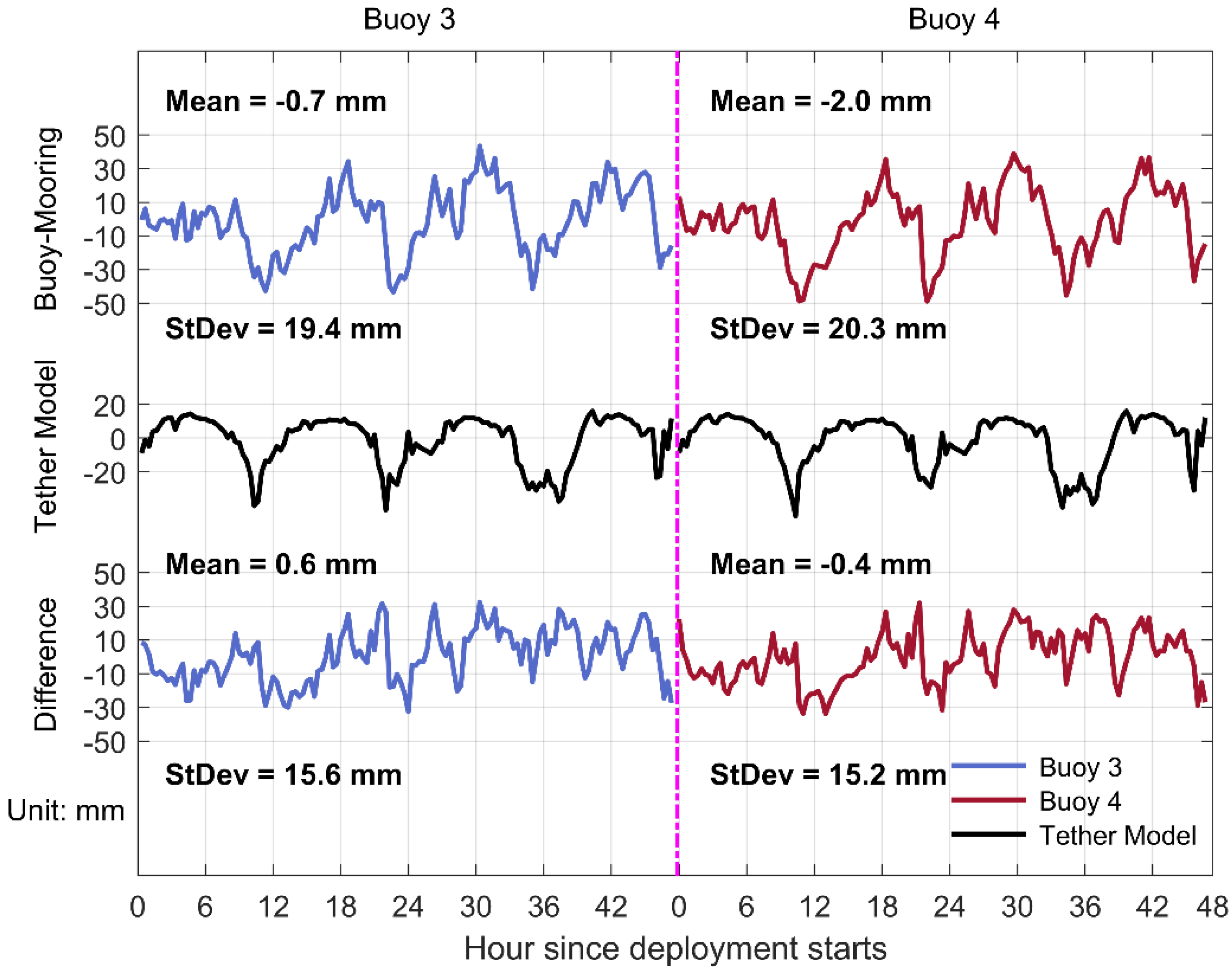
5.3. Case Study: Tether Tension Investigation

Theoretically, the co-located mooring and buoy are sensitive to the same ocean signals and the difference should only contain white noise. However, as demonstrated (Figure S1) there were some deployments with a relatively large periodic residual signal. The upper section of Figure 4 shows this periodic signal for our case study deployment from August 2015. The likelihood of such a signal being introduced by the mooring is small—the bottom pressure sensor is not sensitive to high frequency variability, and the dynamic height component shows negligible periodicity.

Under the assumption that this residual energy is associated predominantly with the GNSS buoy, we sought to empirically model the signal shown in the residual using the current-meter observed currents and ACCESS modelled wind stress. Parameterisation details of the model are provided in Table S4. While the simplistic nature of our model and the limited temporal and spatial resolutions of the input datasets results in relatively high sensitivities in our parameterisation, our model output shows reasonable correlation with the residual in range and in the temporal response for each buoy deployed (middle section, Figure 4). The range (maximum-minus-minimum) of the model and the residual (smoothed using an hourly moving average to match the model sampling) is 60.5 mm and 81.5 mm respectively. The median of the difference in times of peaks between the model and the residual is 22 min which is within the resolution of the hourly data input. Qualitative inspection shows that the model also resolves some of the higher frequency variability (e.g., between 30–42 h for both buoys). Upon the removal of the simulated signal from the residual, the standard deviation is reduced by ~5 mm with obvious attenuation of the low frequency signals and the mean of the residual is brought further to zero for both buoys.

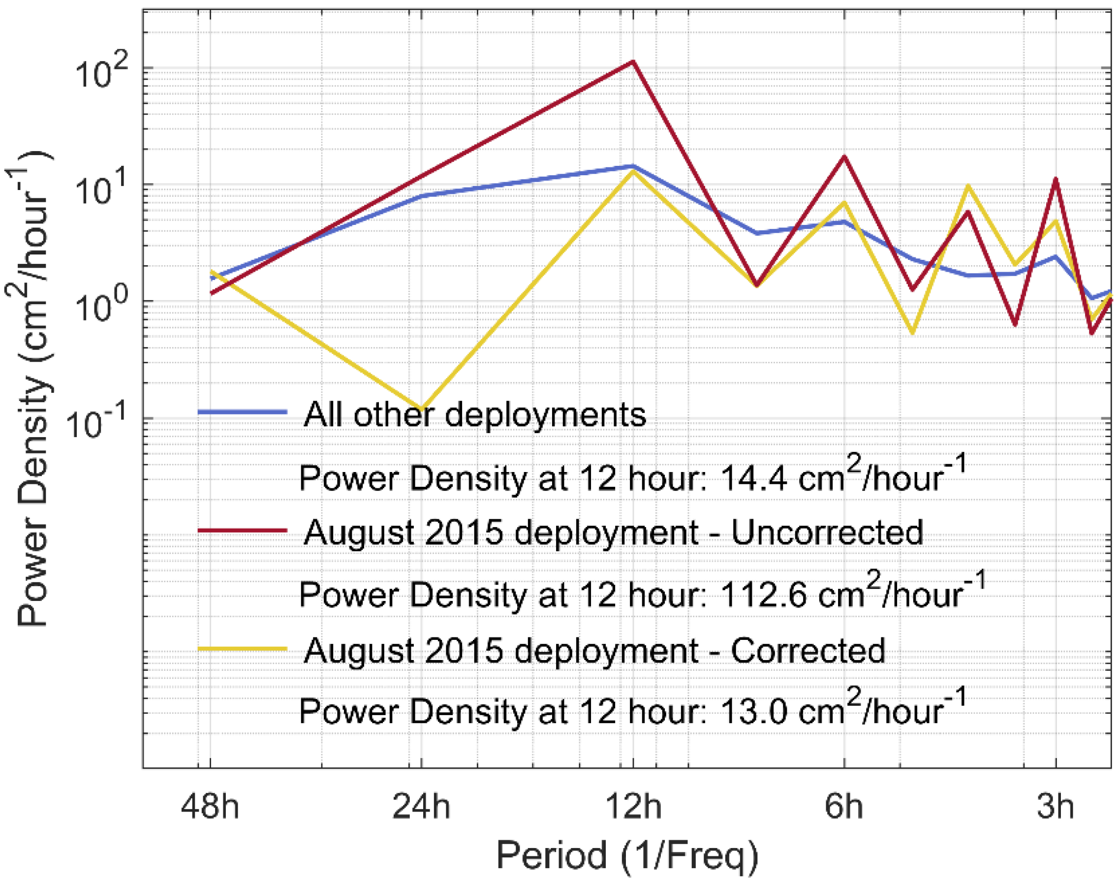
Despite limited low frequency resolution in a ~48-h deployment, the so-called ‘tether tension’ effect is readily apparent in the frequency domain as shown in Figure 5. Here, we see that the August 2015 deployment has an anomalous semi-diurnal signal present in the residual compared with all other available deployments. After applying the modelled signal correction, the power in the ~12-h band was reduced significantly along with some moderate reduction over other low frequency bands as well.

Above the systematic noise baseline of the buoy, we have now shown one possible previously unaccounted factor that can contribute to the overall precision of the buoy system. However, our investigation in this paper is limited to our case study deployment and is not yet applicable for all deployments. Further work is required to understand this effect and we return to possible avenues of investigation in the discussion. One further possible and potentially dominant source of systematic error at higher frequencies is likely because of unmodelled platform orientation—we investigate this issue in the following section.

5.4. Case Study: Modelled Orientation Variation

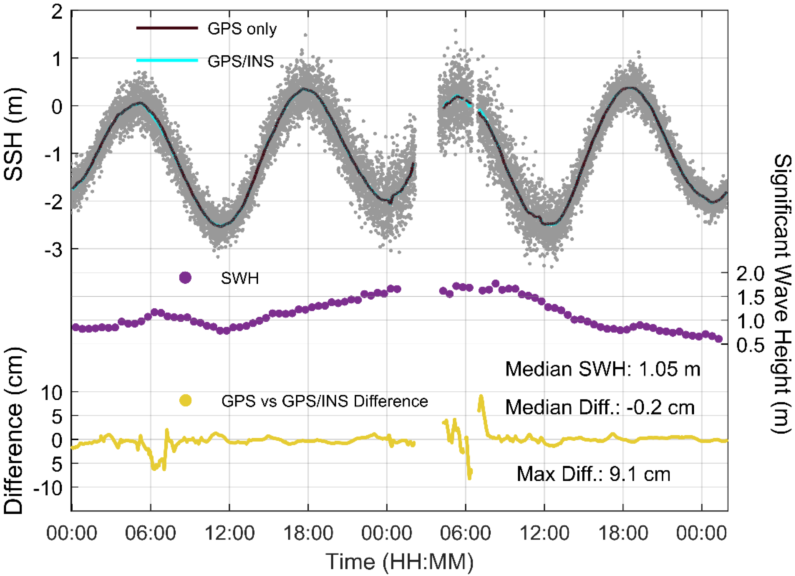
As part of testing new hardware for deployment in the new UTas/IMOS Mk-V buoy system, we were able to integrate an INS unit into our existing Mk-IV system. We use data from a trial deployment in November 2019 to quantify the variation in platform orientation. The top section in Figure 6 shows the GPS/INS processed solution for the trial deployment, where we can see minor variation between GPS only and GPS/INS solutions.

The middle section shows the evolution of significant wave height (SWH) derived from a running 30-min window over the deployment SSH time series. The sea state increases from ~0.75 m to ~1.75 m, returning to a relatively calm ~0.5 m over the deployment. The median SWH is ~1 m, indicating a calm/moderate sea state selected intentionally for standard cal/val deployments at the Bass Strait facility. The bottom section of Figure 6 shows the difference in solutions—both smoothed using a 25 min moving mean smoother prior to differencing. We note that during this relatively calm deployment (see the SWH section and the scatter of the raw GPS/INS solutions in the top section, Figure 6), the difference is usually less than 1 cm. Differences do however reach ~5 cm, when the sea state became rougher around 6 h into the deployment, and as much as ~9 cm during the roughest part of the deployment where loss of lock with satellites was observed possibly due to waves breaking over the relatively low (~0.5 m) Mk-IV antenna.

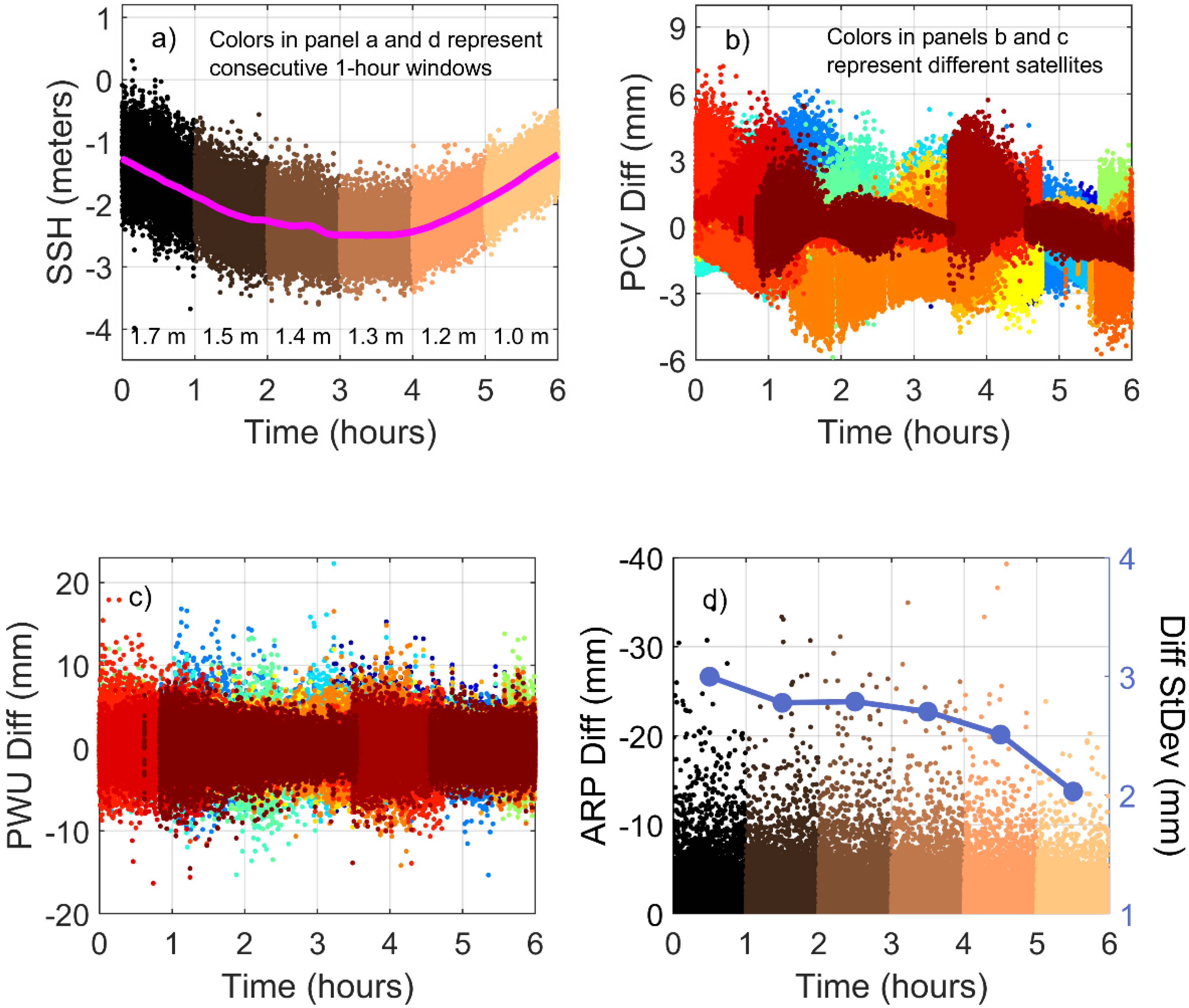
To probe the evolution of orientation variations further, we selected a 6-h session where sea state evolved from moderate to relatively calm (Figure 7a). Figure 7b shows the difference between the GPS only PCV correction on the range and our proposed adaptive PCV correction benefiting from INS data. Here we observe an apparent range in the path-length correction of 9 mm. As the sea state became calmer, the spread of the difference also narrowed to some extent, suggesting a more stable buoy platform.

Satellite-specific plots for GPS only PCV and adaptive GPS/INS PCV are included in the supplementary material (Figure S3), where more obvious platform orientation induced variation can be seen. The difference between static and dynamic phase wrap-up is shown in Figure 7c. Compared with the adaptive PCV, the variation of this term is larger, up to 20 mm when both station and satellite rotations are considered. Inter-comparison plots between static PWU and dynamic PWU are included in the Supplementary Material (Figure S4) in a satellite-specific manner for a more direct comparison between the two terms computed specifically for each satellite. In Figure 7d, the difference between orientation compensated ARP correction and static ARP is shown in corresponding colours to the 1-h window as in Figure 7a. An obvious reduction in the standard deviation of the difference can be observed as the sea states evolves from moderate to calm.

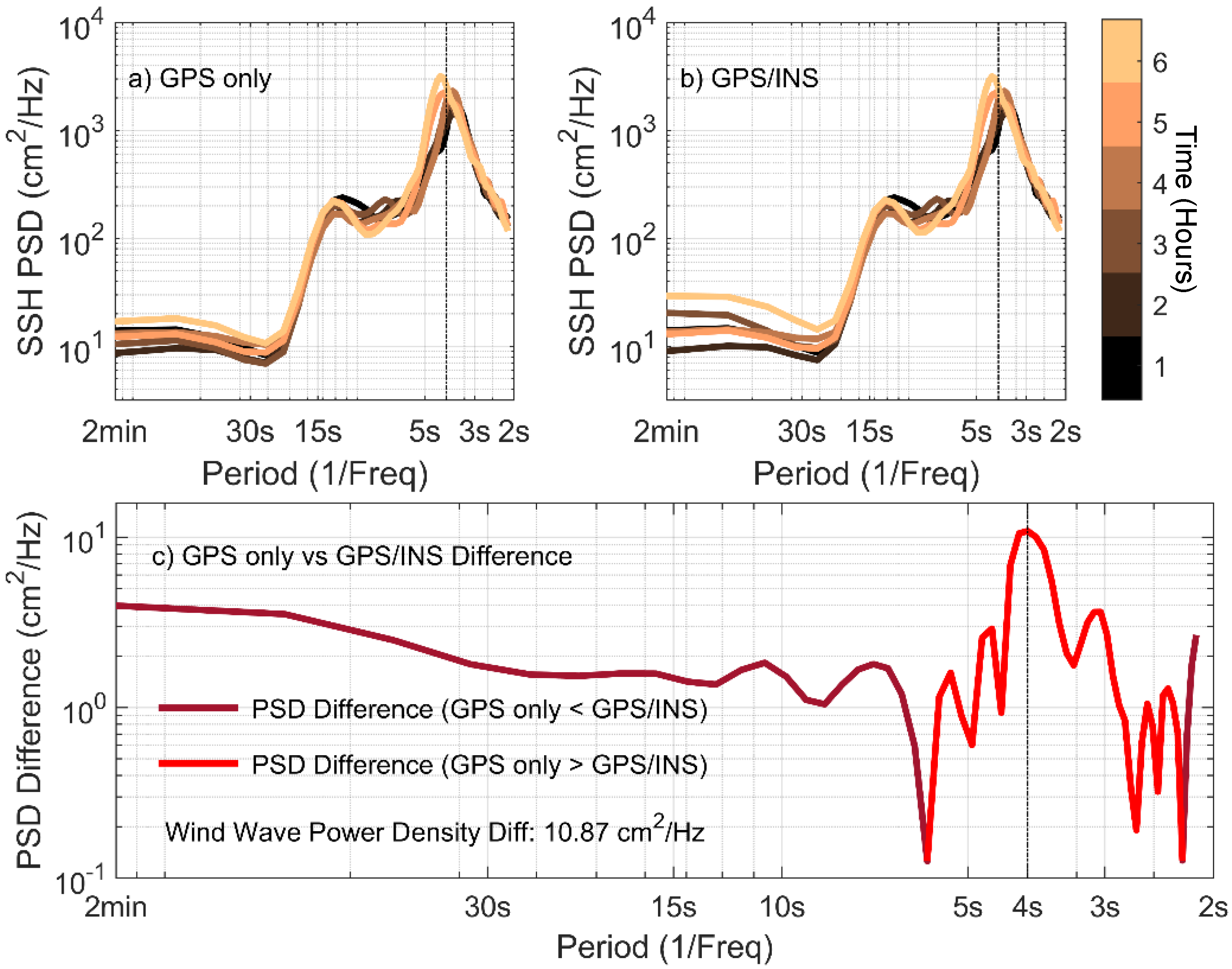
To further investigate the relatively small magnitude variation in GPS only and GPS/INS solutions, we show power density differences within the 2-s to 2-min high frequency band in Figure 8. Within this frequency band, two signals dominate the spectrum—the swell signal band between ~10–14 s and the wind wave band between 3–5 s. In the bottom section of Figure 8, a notable difference is seen between 3 s and 5 s, where the wind waves reside with power density of $10{\mathrm{cm}}^2/\mathrm{Hz}$. This indicates the GPS only residuals have apparent wind wave signals in excess of the GPS/INS solution.

6. Discussion

GNSS-equipped buoys remain a vitally important tool for geometric validation of satellite altimetry. Future wide-swath altimetry missions further elevate the calibration and validation requirements. Understanding the current precision obtainable from an individual buoy and between buoys is therefore essential. Systematic contributions to the buoy error budget must be identified and addressed. Such an advance will benefit present SAR missions (e.g., Sentinel-3A and 3B), the soon to be launched Jason-CS/Sentinel 6 Michael Freilich (end 2020), as well as assist in the preparation for the future interferometric missions (e.g., SWOT).

6.1. Overarching Precision of the UTas/IMOS Mk-IV GNSS Buoy

Thanks to the well archived buoy and co-located mooring datasets from the on-going cal/val activity at the Bass Strait facility, the overarching precision of the buoy system can be assessed. We find a root mean square of the buoy and mooring difference of ~15 mm. Such a precision assessment regards the mooring as a highly reliable in situ ‘ground truth’ which is an assumption with some limitations. Among 27 deployments that we have assessed, one deployment (September 2016) was excluded as an outlier given a mean bias of 44 mm (Table S3). Whether this offset was induced from the mooring or buoy data remains unknown—the mooring cannot be excluded given the potential for temporary fouling of conductivity sensors leading to short-term biases in the dynamic height correction. This highlights that our statistics of the overarching precision includes a contribution from the in situ ‘ground truth’ and is not solely limited to the GNSS-equipped buoy.

Among all deployments we assessed, there were some deployments (Figure S1) with noticeable systematic signals like those evident in the August 2015 deployment investigated for the tether tension effect. These systematic signals have energy in the semi-diurnal tidal band with an amplitude of up to 2 cm. While contribution from the mooring time series cannot be excluded entirely, we suspect that such a periodic signal is most likely related to the variation in buoyancy position of the buoy as function of dynamic changes in the tension of the tension caused by waves and currents. In the context of the cal/val requirements for the future SWOT mission, this presents one of the key motivations for this paper and the simultaneous development of the UTas/IMOS Mk-V buoy. Left unattended, these systematic biases may limit the potential contribution to ocean tidal modelling or SSH validation at frequencies in the tidal band.

The historical buoy dataset at Bass Strait also offered us a unique opportunity to investigate systematic errors within the buoy system from a GPS processing prospective. The assumption involved in this comparison is that by making the difference between measured SSH from the dual-buoy setup, most external factors affecting precision will cancel out. However, since there is still a practical physical distance between two buoys, certain high frequency yet spatially decorrelated signals (e.g., wind waves, swell) should be filtered out before such an assessment. Hence, with a 25-min moving mean filter, we determine a noise baseline of 8.5 mm (Figure 3) for the UTas/IMOS Mk-IV buoy system as used in routine operations at the Bass Strait validation facility. Whether the 25-min moving mean filter is the most appropriate is an open and important question.

The difference between the SSH and δSSH precision metrics (~15 mm vs. ~8.5 mm respectively) prompted our investigation into possible unmodelled effects for the current buoy setup. Buoyancy displacement caused by external forcing and the variation in buoy platform orientation were two key issues investigated.

6.2. Buoyancy Displacement

GNSS buoys for altimetry validation are typically required to be constrained to the near vicinity of a comparison point using a horizontal tether attached to a float that is subsequently anchored to the sea floor. This provides the benefit of securing the scientific equipment and also guarantees measurements taken close enough to the comparison point of interest. This comes with the disadvantage of inducing time variable tension on the tether as a function of external forcing such as currents, surface wind, waves etc. This leads to the self-adjustment of the buoy buoyancy inducing non-linear signals into the SSH solution. For the majority of the 27 deployments investigated from the Bass Strait facility, this signal is typically small (<10 mm) which is likely as a result of relatively calm sea states during deployment and the hydrodynamic properties of the UTas/IMOS Mk-IV buoy. However, a small number of deployments show spurious residuals with energy in the semi-diurnal tidal band suggesting some effect correlated with the tide or tidal currents which are predominately semi-diurnal in nature across Bass Strait.

From the limited dataset we can assemble using current-meter data and hindcast modelled wind stress, our empirically modelled signal shows reasonable agreement with the dominant periodic low frequency signal band of the residual (Figure 4). Applying our model reduces the variability of the variance in the residual by a significant amount (RMS reduced from ~20 mm to ~15 mm corresponding to a variance reduction of ~40%). However, because of the limited temporal and spatial resolution of our input data, only the low frequency components of the residual signal were attenuated effectively. The difference still contains variability suggesting that further effort here may be beneficial. From the perspective of our model input data, the current fields are dominated by semi-diurnal periodicity, hence can only replicate part of the residual signal observed, while wind stress is usually irregular and progresses in a Gauss-Markov manner over the same period of time. In retrospect, the random walk feature of the wind stress input helped to some extent modelling the high frequency response of the tether where abrupt short-term changes were observed (Figure 4). However, to provide further noticeable difference towards the high frequency bands, higher resolution input is needed.

When comparing this deployment to the in situ mooring time series, it is important to note how the mean biases of two separate buoys had been brought closer towards zero using the tether tension model. Moreover, we noticed a reduced asymmetry in distribution of the residuals after the correction (Figure S2), which may be an indicator that the tether model helped to restore the normal distribution of the residual to some extent, leveling out the general in-ward tilting of the buoy relative to the tether during the deployment. Whilst it is difficult to assess the statistical significance of such an effect, the improvement adds weight to our model having some skill in quantifying the variation of buoyancy position.

While our tether tension modelling is simplistic and limited by the spatial and temporal resolution of the input data, the power density reduction shown in Figure 5 shows promise. Power density over low frequency bands of the buoy minus mooring residual was reduced by 51%, though energy towards higher frequencies could possibly be further improved if higher spatiotemporal resolution data can be achieved as input. Although the model fits the August 2015 deployment relatively well, it is not globally applicable to other deployments noting further testing and development is required. This indicates one condition attached to our trial model: tension on the tether has to be significant enough to yield a reasonable Signal-Noise-Ratio (SNR) in the residual. This further implies two potential improvements for the model: better formulation of Equation (7) to reduce parameter sensitivity towards input; and including higher resolution input data.

In the context of SWOT validation at the Bass Strait facility, improved understanding of the tether tension effect will be possible given the planned co-location of new GNSS Mk-V buoys with 5-beam ADCP instruments operating as a shallow water current, waves and pressure inverted echo sounder (CWPIES). This system will observe not only SSH (with arbitrary datum) but surface currents and directional wave data [42]. Combined, these data offer significant potential to further improve our empirical tether tension model which we note will be specific to the hydrodynamic properties of the Mk-V buoy design. Coupled with high resolution ocean and atmospheric modelling over the Bass Strait domain, we see significant potential to further improve from the initial investigation presented here.

6.3. Variation in Buoy Platform Orientation

Another unmodelled but essential consideration for buoy processing is the variation in platform orientation. With constant and ever-changing forcing applied on the buoy, high frequency motions of the buoy are expected and include rotation and horizontal pitching and rolling. This breaks the usual assumption of conventional GNSS processing where the antenna remains upright and fixed with respect to the Earth. The violation of such an assumption dictates that platform orientation must be considered when high precision solutions are required.

It should be noted that the estimation of the platform orientation is usually a requirement in airborne and spaceborne platform positioning and navigation [43,44], where the air/spacecraft has nonholonomic constraints or need to be a strict holonomic system. For our buoy deployments, although the waterbody supports and provides the buoy with a quasi-holonomic constraint to some extent, it also has a “non-rigid” characteristic that induces the variation in orientation. Both aspects to this issue work in favour of our buoy. First, the quasi-holonomic constraint limits the buoy motion and helps maintain a quasi-normal distribution of orientation induced biases—most evident in Figure S4. Additionally, the quasi-free drifting motion (while tethered) helps channel the energy from the ocean with only small influence on the mean buoyancy location.

However, there are some limitations caused by the nature of the buoy motion. We note the buoy usually moves at horizontal velocities of ~0.2 m/s during typical deployments which have relatively low sea states. Since our INS unit is MEMS grade, under low velocity scenarios, it cannot generate an acceptable SNR for conventional GNSS/INS integration (e.g., [45,46]). To compensate, we took advantage of the magnetometer onboard the INS unit and applied a 9-DOF (i.e., 3-axis gyroscope, 3-axis accelerometer, 3-axis magnetometer) filter to derive platform orientations. Orientation solutions were then passed to the GNSS processing to apply orientation corrections at observation level, which further helped ambiguity resolution along the processing flow.

Our results from using our enhanced TRACK processing suite suggest that the differences between GPS only and GPS/INS SSH solutions are non-trivial at the cm level (Figure 6), signifying the importance of platform orientations. At the observation level, adaptive PCV and dynamic PWU may bias the theoretical range during ambiguity resolution up to a magnitude of 1 cm and 2 cm respectively (Figure 7) under relatively low sea states (SWH = 1 m). These biases will undoubtedly scale with increasing sea state.

The orientation compensated ARP is a more direct but larger magnitude correction to the measured SSH. For the previous buoy deployment processing for the Bass Strait validation activities, the ARP was considered as a constant offset and was directly applied during postprocessing procedures. This simply ignores the antenna motion at sea and the reduced height was an approximation of the instantaneous SSH. While a large proportion of this bias can be eliminated, there is certain part of the bias that will not be ‘averaged’ out causing a systematic difference in the solution. This is because the “true” ARP correction in the vertical component is always smaller than the “constant” ARP value at sea and the antenna seldom returns to its upright position. From Figure 7 we can infer that the ARP bias for the historical buoy solution (using the Mk-IV buoys) is highly likely to be within a range of 0 to +5 mm in typical sea states of SWH 0.5–1 m. This bias will increase for the newer Mk-V buoys given an increase in antenna to nominal water level distance from ~0.5 m to ~1.0 m.

In the frequency domain, the power density difference (Figure 8) showed a significant peak between the 3–5 s period band. This is an important point—the enhanced processing reduces high frequency biases, with improvements of ~10 ${\mathrm{cm}}^2/\mathrm{Hz}$. Such improvement may assist us understand the energy evolution between swell and wind waves better. We note, however, that the use of GNSS-equipped buoys to characterise the true high frequency sea state is dependent on the hydrodynamic properties of the buoy.

Although our GPS/INS solution showed some differences in the temporal and frequency domain compared with the GPS only solution, we are not yet able to formally quantify the orientation induced biases on the historical deployments because they lacked an INS instrument. We require further deployments with the new Mk-V buoy design deployed with co-located CWPIES and conventional mooring SSH to fully understand the performance of the Mk-V design. This will include the assessment of the inclusion of INS data for improved ambiguity resolution.

6.4. Implication for Ocean Process Studies

The capability of present-day altimetry missions limits our ability to study ocean processes under spatial scales of 200 km. This is primarily due to the satellite ground track separation and partially because of the along-track footprint resolution. SWOT holds the potential of overcoming the limitation of ground track separation associated with present-day missions and will eventually enable us to probe into meso- to sub-mesoscale ocean processes which evolve at spatial scales below 200 km.

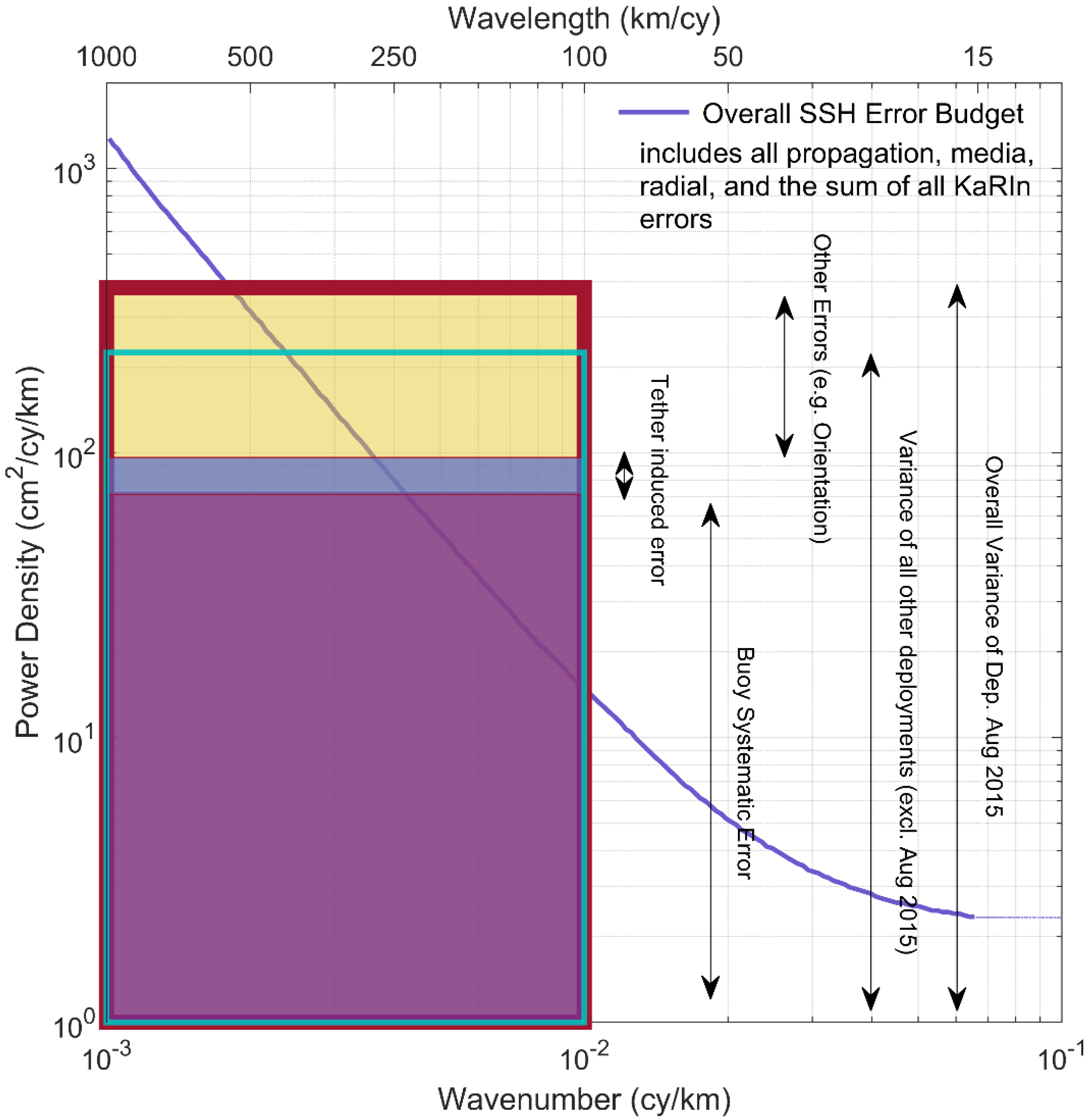
To prepare for the mission, the SWOT science definition team generated an empirically derived set of scientific requirements spanning a full range of ocean processes ranging in wavelength from 15 km to 1000 km (Figure 8). The requirements are prescribed in the spatial frequency domain or wavenumber space as directly linked to the wavelength of ocean process under investigation.

This offers us the opportunity to map our present-day buoy precision onto the SWOT requirement spectrum and discuss the implications for both buoy development and SWOT validation. Using our case study deployment for tether tension modelling, we were able to generate comparative components on the wavenumber spectrum (Text S2) in Figure 9. However, it should be clear that our discussion here transforms point-based buoy precision onto a wavenumber spectrum from an integrated variance perspective. It does not indicate power density corresponding to any wavenumber. As a result, we selectively mapped against wavelength of 100 km simply for comparative purposes (Figure 9).

The outer rectangular box in Figure 9 indicates a 19.5 mm RMS of the buoy against mooring residual from the August 2015 deployment. Inside it, the purple area shows the systematic noise we have assessed from dual-buoy system analysis, which is 8.5 mm. The thin blue area in the middle is from the tether tension model. We used 5 mm from the standard deviation reduction. All other remaining error sources (including the orientational error) are coloured yellow. The area enclosed by cyan lines indicates the overarching precision of 15 mm derived from all other deployments (excluding August 2015).

From Figure 9 it is obvious that the present-day Mk-IV buoy system does not meet the precision requirements for studying ocean processes at spatial scales of 100 km as represented by the purple line. However, our work here identifies significant scope for improvement. First, systematic error may be further reduced with the improved observational model adopted, the addition of other GNSS constellations (e.g., GLONASS) and INS integration at the observational level to improve ambiguity resolution. With reference to Figure 9, these changes will reduce the yellow and purple areas respectively. Second, improvements to the tether tension model as discussed earlier will contract the blue area in the figure, and further reduce the yellow area. The proposed UTas/IMOS Mk-V buoy system currently under development aims to address and mitigate these issues.

7. Conclusions

Both the overarching and relative precision of the present-day Mk-IV buoy system at the Bass Strait altimeter validation facility was assessed using an existing archived dataset. Using over 2000 h of 1 Hz GNSS buoy deployment data, we were able to quantify the overarching precision of the buoy to be approximately 15 mm. Analysis of dual-buoy deployments enabled the determination of the systematic error of the buoys at 8.5 mm. In the context of the demanding validation requirements for future altimeter missions, we sought to find avenues for improvement.

Through a careful examination of the buoy data and assessment of the actual deployment configuration, we further identified two key previously unaddressed issues; namely buoyancy displacement caused by the tether tension and bias induced by unmodelled changes in platform orientation. Our first attempt at an empirical model to address tether tension showed promising results with a strong correlation between currents, wind stress and buoy SSH residual against the in situ mooring time series. Our simple empirical model was able to reduce the power density over low frequency bands (up to 6 h) of the residuals by ~51% corresponding to an overall ~5 mm RMS reduction in the residual, though limited in part by the insufficient resolution of input data. Significant scope to further improve this result was identified with the future co-location of GNSS-equipped buoys and coastal CWPIES instruments, together with higher resolution wave and atmospheric modelling. INS integration was proven to be a necessity as all three unmodelled variations associated with platform orientation combined with a magnitude at the 1 cm level in the final GPS/INS solutions. Under sea states with SWH >1 m, these three variations will induce even higher magnitude of biases if left uncorrected.

As the international community awaits interferometric wide-swath altimetry with the planned launch of SWOT in 2022, further preparations like those presented here are required to meet the demanding validation requirements of such missions. With the present-day transition from LRM to SAR altimetry, we are offered an opportunity to improve our understanding of both altimeter and in situ observations of the sea surface and thus improve oceanographic interpretation. GNSS-equipped buoys remain an important tool in this endeavour.

References

- Fu, L.-L.; Cazenave, A. Satellite Altimetry and Earth Sciences: A Handbook of Techniques and Applications; Academic Press: London, UK, 2000. [Google Scholar]
- Ablain, M.; Cazenave, A.; Larnicol, G.; Balmaseda, M.; Cipollini, P.; Faugère, Y.; Fernandes, M.J.; Henry, O.; Johannessen, J.A.; Knudsen, P.; et al. Improved sea level record over the satellite altimetry era (1993–2010) from the Climate Change Initiative project. Ocean. Sci. 2015, 11, 67–82. [Google Scholar] [CrossRef]
- Nerem, R.S.; Beckley, B.D.; Fasullo, J.T.; Hamlington, B.D.; Masters, D.; Mitchum, G.T. Climate-change-driven accelerated sea-level rise detected in the altimeter era. Proc. Natl. Acad. Sci. USA 2018, 115, 2022–2025. [Google Scholar] [CrossRef] [PubMed]
- Stammer, D.; Wunsch, C. Preliminary assessment of the accuracy and precision of TOPEX/POSEIDON altimeter data with respect to the large-scale ocean circulation. J. Geophys. Res. Space Phys. 1994, 99, 24584. [Google Scholar] [CrossRef]
- Stammer, D. Global characteristics of ocean variability estimated from regional TOPEX/POSEIDON altimeter measurements. J. Phys. Oceanogr. 1997, 27, 1743–1769. [Google Scholar]
- Fu, L.-L.; Chelton, D.; Le Traon, P.-Y.; Morrow, R. Eddy Dynamics from Satellite Altimetry. Oceanography 2010, 23, 14–25. [Google Scholar] [CrossRef]
- Fiedler, M.; Adler, L.; Young, C.L. Health Care in President Trump’s Fiscal Year 2021 Budget. JAMA Health Forum 2020, 1, e200181. [Google Scholar] [CrossRef]
- Morrow, R.; Fu, L.-L.; Ardhuin, F.; Benkiran, M.; Chapron, B.; Cosme, E.; D’Ovidio, F.; Farrar, J.T.; Gille, S.T.; Lapeyre, G.; et al. Global Observations of Fine-Scale Ocean Surface Topography With the Surface Water and Ocean Topography (SWOT) Mission. Front. Mar. Sci. 2019, 6. [Google Scholar] [CrossRef]
- Fernandez, D.E.; Fu, L.; Pollard, B.; Vaze, P.; Abelson, R.; Nathalie, S. SWOT Project Mission Performance and Error Budget; Jet Propulsion Laboratory Document D-79084 Revision A: Pasadena, CA, USA, 2017. [Google Scholar]
- Bonnefond, P.; Exertier, P.; Laurain, O.; Jan, G. Absolute Calibration of Jason-1 and Jason-2 Altimeters in Corsica during the Formation Flight Phase. Mar. Geod. 2010, 33, 80–90. [Google Scholar] [CrossRef]
- White, N.J.; Coleman, R.; Church, J.A.; Morgan, P.J.; Walker, S.J. A southern hemisphere verification for the TOPEX/POSEIDON satellite altimeter mission. J. Geophys. Res. Space Phys. 1994, 99, 24505. [Google Scholar] [CrossRef]
- Watson, C.S.; Coleman, R.; White, N.; Church, J.A.; Govind, R. Absolute Calibration of TOPEX/Poseidon and Jason-1 Using GPS Buoys in Bass Strait, Australia Special Issue: Jason-1 Calibration/Validation. Mar. Geod. 2003, 26, 285–304. [Google Scholar] [CrossRef]
- Watson, C.S.; White, N.; Coleman, R.; Church, J.; Morgan, P.; Govind, R. TOPEX/Poseidon and Jason-1: Absolute Calibration in Bass Strait, Australia. Mar. Geod. 2004, 27, 107–131. [Google Scholar] [CrossRef]
- Watson, C.S. Satellite Altimeter Calibration and Validation Using GPS Buoy Technology. Ph.D. Thesis, University of Tasmania, Burnie, Tasmania, 2005. [Google Scholar]
- Watson, C.S.; White, N.; Church, J.A.; Burgette, R.; Tregoning, P.; Coleman, R. Absolute Calibration in Bass Strait, Australia: TOPEX, Jason-1 and OSTM/Jason-2. Mar. Geod. 2011, 34, 242–260. [Google Scholar] [CrossRef]
- Watson, C.; White, N.; Burgette, R.; Coleman, R.; Church, J.; Zhang, J. In Situ Calibration Results from Bass Strait. In Proceedings of the OSTST Meeting, Seattle, WA, USA, 22–24 June 2009. [Google Scholar]
- Hein, G.W.; Landau, H.; Blomenhofer, H. Determination of instantaneous sea surface, wave heights, and ocean currents using satellite observations of the global positioning system. Mar. Geod. 1990, 14, 217–224. [Google Scholar] [CrossRef]
- Kelecy, T.; Born, G.; Röcken, C. GPS buoy and pressure transducer results from the August 1990 Texaco Harvest Oil Platform Experiment. Mar. Geod. 1992, 15, 225–243. [Google Scholar] [CrossRef]
- Born, G.H.; Parke, M.E.; Axelrad, P.; Gold, K.L.; Johnson, J.; Key, K.W.; Kubitschek, D.G.; Christensen, E.J. Calibration of the TOPEX altimeter using a GPS buoy. J. Geophys. Res. Space Phys. 1994, 99, 24517. [Google Scholar] [CrossRef]
- Bonnefond, P.; Exertier, P.; Laurain, O.; Ménard, Y.; Orsoni, A.; Jeansou, E.; Haines, B.J.; Kubitschek, D.G.; Born, G. Leveling the Sea Surface Using a GPS-Catamaran Special Issue: Jason-1 Calibration/Validation. Mar. Geod. 2003, 26, 319–334. [Google Scholar] [CrossRef]
- Fund, F.; Perosanz, F.; Testut, L.; Loyer, S. An Integer Precise Point Positioning technique for sea surface observations using a GPS buoy. Adv. Space Res. 2013, 51, 1311–1322. [Google Scholar] [CrossRef]
- Maqueda, M.A.M.; Penna, N.T.; Williams, S.; Foden, P.R.; Martin, I.; Pugh, J. Water Surface Height Determination with a GPS Wave Glider: A Demonstration in Loch Ness, Scotland. J. Atmos. Ocean. Technol. 2016, 33, 1159–1168. [Google Scholar] [CrossRef]
- Penna, N.T.; Maqueda, M.A.M.; Martin, I.; Guo, J.; Foden, P.R. Sea Surface Height Measurement Using a GNSS Wave Glider. Geophys. Res. Lett. 2018, 45, 5609–5616. [Google Scholar] [CrossRef]
- Haines, B.; Desai, S.; Dodge, A.; Meinig, C.; Leben, B.; Shannon, M. The Harvest Experiment: New Results from the Platform and Moored GPS Buoys [Poster Presentation]. In Proceedings of the Ocean Surface Topography Science Team (OSTST) Meeting, Chicago, IL, USA, 21–25 October 2019. [Google Scholar]
- De Vries, J.J.; Waldron, J.; Cunningham, V. Field tests of the new Datawell DWR-G GPA wave buoy. Sea Technol. 2003, 44, 50–55. [Google Scholar]
- Jeans, G.; Bellamy, I.; de Vries, J.J.; Van Weert, P. Sea trial of the new Datawell GPS directional Waverider. In Proceedings of the IEEE/OES Seventh Working Conference on Current Measurement Technology, San Diego, CA, USA, 13–15 March 2003. [Google Scholar]
- Datawell BV. Datawell Waverider Reference Manual. Datawell BV Zumerlustraat 2006, 4, 2012. [Google Scholar]
- Farnell. MTi User Manual 2018, MTi 10-series and MTi 100-series 5th Generation, Document MT0605P, Revision 2018.A; Xsens Technologies: Culver City, CA, USA, 2018. [Google Scholar]
- BoM, A. Operational implementation of the ACCESS Numerical Weather Prediction systems. NMOC Oper. Bull. 2010, 83, 12. [Google Scholar]
- TRACK MIT. GPS Differential Phase Kinematic Positioning Program; Delft University of Technology: Delft, The Netherlands, 2011. [Google Scholar]
- Kouba, J. Implementation and testing of the gridded Vienna Mapping Function 1 (VMF1). J. Geod. 2007, 82, 193–205. [Google Scholar] [CrossRef]
- Petit, G.; Luzum, B. IERS Conventions; Bureau International des Poids et Mesures: Sevres, France, 2010. [Google Scholar]
- Zhu, S.Y.; Groten, E. Relativistic effects in GPS. GPS-Techniques Applied to Geodesy and Surveying; Springer: Berlin/Heidelberg, Germany, 1988; pp. 41–46. [Google Scholar]
- Landskron, D.; Böhm, J. VMF3/GPT3: Refined discrete and empirical troposphere mapping functions. J. Geod. 2018, 92, 349–360. [Google Scholar] [CrossRef] [PubMed]
- Berrisford, P.; Dee, D.; Poli, P.; Brugge, R.; Fielding, K.; Fuentes, M.; Kallberg, P.; Kobayashi, S.; Uppala, S.; Simmons, A. The ERA-Interim Archive, Version 2.0; ECMWF: Shinfield Park, Reading, UK, 2011. [Google Scholar]
- Boehm, J.; Werl, B.; Schuh, H. Troposphere mapping functions for GPS and very long baseline interferometry from European Centre for Medium-Range Weather Forecasts operational analysis data. J. Geophys. Res. Sol. Earth 2006, 111, 406. [Google Scholar] [CrossRef]
- Madgwick, S. An efficient orientation filter for inertial and inertial/magnetic sensor arrays. Rep. X-IO Univ. Bristol 2010, 25, 113–118. [Google Scholar]
- Van Loan, C.F.; Golub, G.H. Matrix Computations; Johns Hopkins University Press: Baltimore, MD, USA, 1983. [Google Scholar]
- Rauch, H.E.; Tung, F.; Striebel, C.T. Maximum likelihood estimates of linear dynamic systems. AIAA J. 1965, 3, 1445–1450. [Google Scholar] [CrossRef]
- Wu, J.-T.; Wu, S.C.; Hajj, G.A.; Bertiger, W.I.; Lichten, S.M. Effects of antenna orientation on GPS carrier phase. ASDY 1992, 1647–1660. [Google Scholar]
- Brook, R.J.; Arnold, G.C. Applied Regression Analysis and Experimental Design; Informa UK Limited: London, UK, 2018. [Google Scholar]
- Legresy, B.; Watson, C.; Carentz, S. CWPIES, a shallow water current, waves and pressure inverted echo sounder for higher resolution satellite altimetry calibration and validation [Poster presentation CVL_002]. In Proceedings of the Ocean Surface Topography Science Team (OSTST) Meeting, Chicago, IL, USA, 21–25 October 2019. [Google Scholar]
- Kim, S.-G.; Crassidis, J.L.; Cheng, Y.; Fosbury, A.M.; Junkins, J.L. Kalman Filtering for Relative Spacecraft Attitude and Position Estimation. J. Guid. Control. Dyn. 2007, 30, 133–143. [Google Scholar] [CrossRef]
- Watson, R.M.; Gross, J.N.; Bar-Sever, Y.; Bertiger, W.I.; Haines, B.J. Flight data assessment of tightly coupled PPP/INS using real-time products. IEEE Aerosp. Electron. Syst. Mag. 2017, 32, 10–21. [Google Scholar] [CrossRef]
- Shin, E.-H. Accuarcy Improvement of Low Cost INS/GPS for Land Applications. Master’s Thesis, University of Calgary, Calgary, AB, Canada, 2001. [Google Scholar]
- Shin, E.-H. Estimation Techniques for Low-Cost Inertial Navigation; UCGE Report 20219. Ph.D. Thesis, University of Calgary, Calgary, AB, Canada, 2005. [Google Scholar]
Figure 1.
Detailed view of the Bass Strait altimeter validation facility. Existing comparison points (CPs) for the Jason-series, Sentinel-3A and Sentinel-3B missions are shown as coloured dots. Buoy 3, Buoy 4 and the mooring from the deployments investigated in this paper were deployed at the JAS CP (red). Mission ground tracks shown as coloured lines. The SWOT 1-day repeat fast sampling orbit is shown in yellow (swath limits shown as solid lines, centre nadir altimeter shown as a dashed line). Note the red line indicates the Jason-series ground track also to be used for the Sentinel-6 Michael Freilich mission.
Figure 2.
Distribution of summary statistics derived from buoy against mooring residuals. StDev stands for standard deviation. Blue histogram shows the distribution of deployment-wise means of residuals; Yellow histogram shows the distribution of deployment-wise standard deviations. A total number of 27 deployments, 2015 h of data is used in the histogram.
Figure 3.
Histogram of δSSH between both buoys deployed in close proximity at the Bass Strait Jason-series comparison point. StDev stands for standard deviation. A total number of 645-h 1 Hz GPS data was involved.
Figure 4.
Residual investigation for the August 2015 deployment; Upper section: SSH residual between buoy and mooring; Middle section: simulated signal as a function of current and wind stress; Lower section: difference between tether modelled SSH residual and measured SSH residual; StDev stands for standard deviation; Vertical line is to separate Buoy 3 and Buoy 4 solutions in the same deployment.
Figure 5.
Power spectrums of buoy-mooring SSH residual. Blue line is the median spectrum for residuals from all the other deployments excluding August 2015, all with less apparent quasi-semi-diurnal signals; Red line is the raw August 2015 deployment residuals; Yellow line is following correction using the empirical model. Note the focus of this figure is on the low frequency bands, hence only these bands are shown.
Figure 6.
Inter-comparison between GPS only and GPS/INS solutions; Grey dots show the 15 s sub-samples from raw 2 Hz GPS/INS solutions; Black and cyan lines show respectively the 25-min moving mean solutions from GPS only and GPS/INS (note these two lines are largely indistinguishable in the top panel); Purple dots show SWH computed from raw SSH solutions over a running 30-min window for the deployment; Yellow line shows the difference between GPS only and GPS/INS SSH solutions.
Figure 7.
GPS/INS solution and orientational variation from a selected session window; (a) SSH showing decreasing sea state over consecutive 1-h sessions colored accordingly. Dots show the raw SSH, the solid magenta line shows the smoothed SSH with a 25-min moving mean; the number annotated at the bottom of (a) indicates the SWH computed over corresponding 1-h window; (b) difference between adaptive PCV and static PCV for all satellites (colored accordingly) involved within the same time window, taken as adaptive minus static; (c) difference between dynamic PWU and static PWU for all satellites involved within the same time window, taken as dynamic minus static; (d) Difference between orientation compensated ARP and static ARP for the same time window, taken as orientation compensated minus static; blue line shows the standard deviation (StDev) of the difference.
Figure 8.
High frequency Power Spectrum Density (PSD) of GPS only (a) and GPS/INS SSH (b) solutions; Panel (c) shows differences of PSD between GPS only and GPS/INS, taken as the absolute value of GPS only minus GPS/INS, but marked in different colours to show which solution has the dominant noise; Vertical thin black line indicates maximum PSD difference; Colormap indicates six consecutive 1-h windows for the upper panel of (a,b).
Figure 9.
SWOT wave-number spectrum requirement with buoy deployment derived error sources mapped arbitrarily to the 100 km wavelength.
© 2020 by the authors. Licensee MDPI, Basel, Switzerland. This article is an open access article distributed under the terms and conditions of the Creative Commons Attribution (CC BY) license (http://creativecommons.org/licenses/by/4.0/).