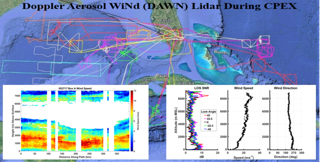
Doppler Aerosol WiNd (DAWN) Lidar during CPEX 2017: Instrument Performance and Data Utility


Abstract

1. Introduction
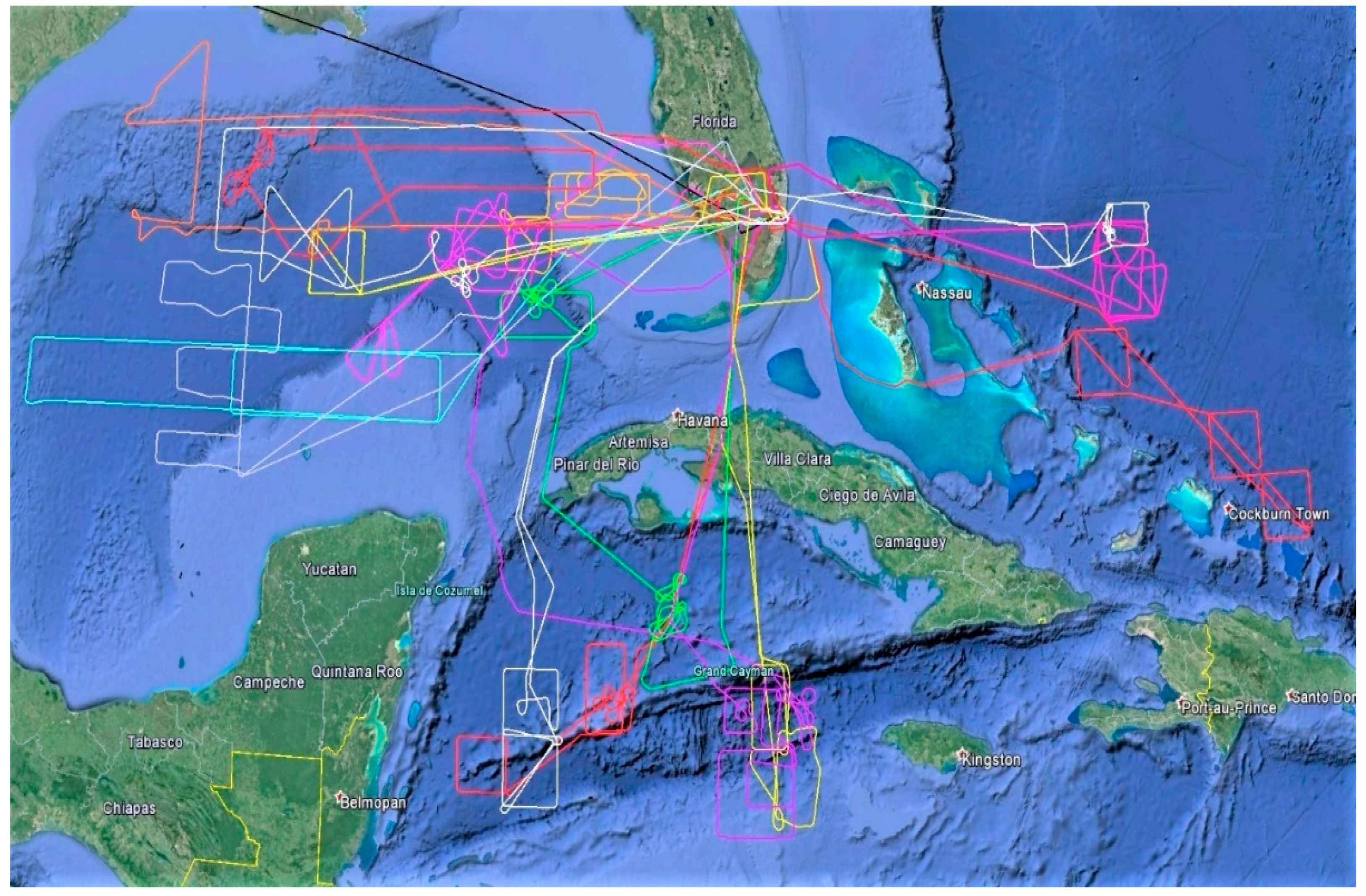
2. Field Campaign
3. The DAWN Instrument and Wind Data Retrieval Methods
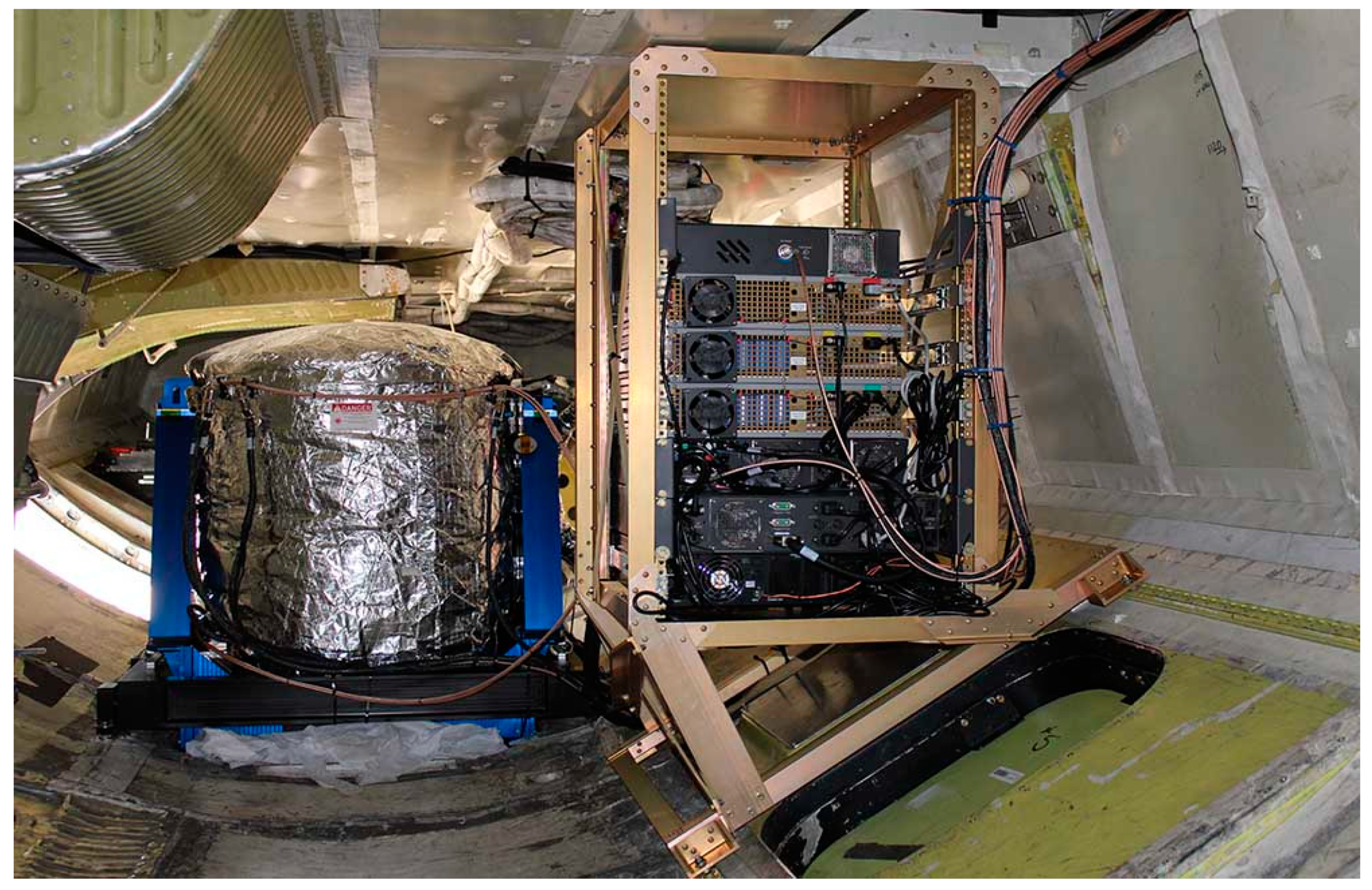
3.1. DAWN Instrument Description
3.2. DAWN Wind Data Retrieval and Data Products
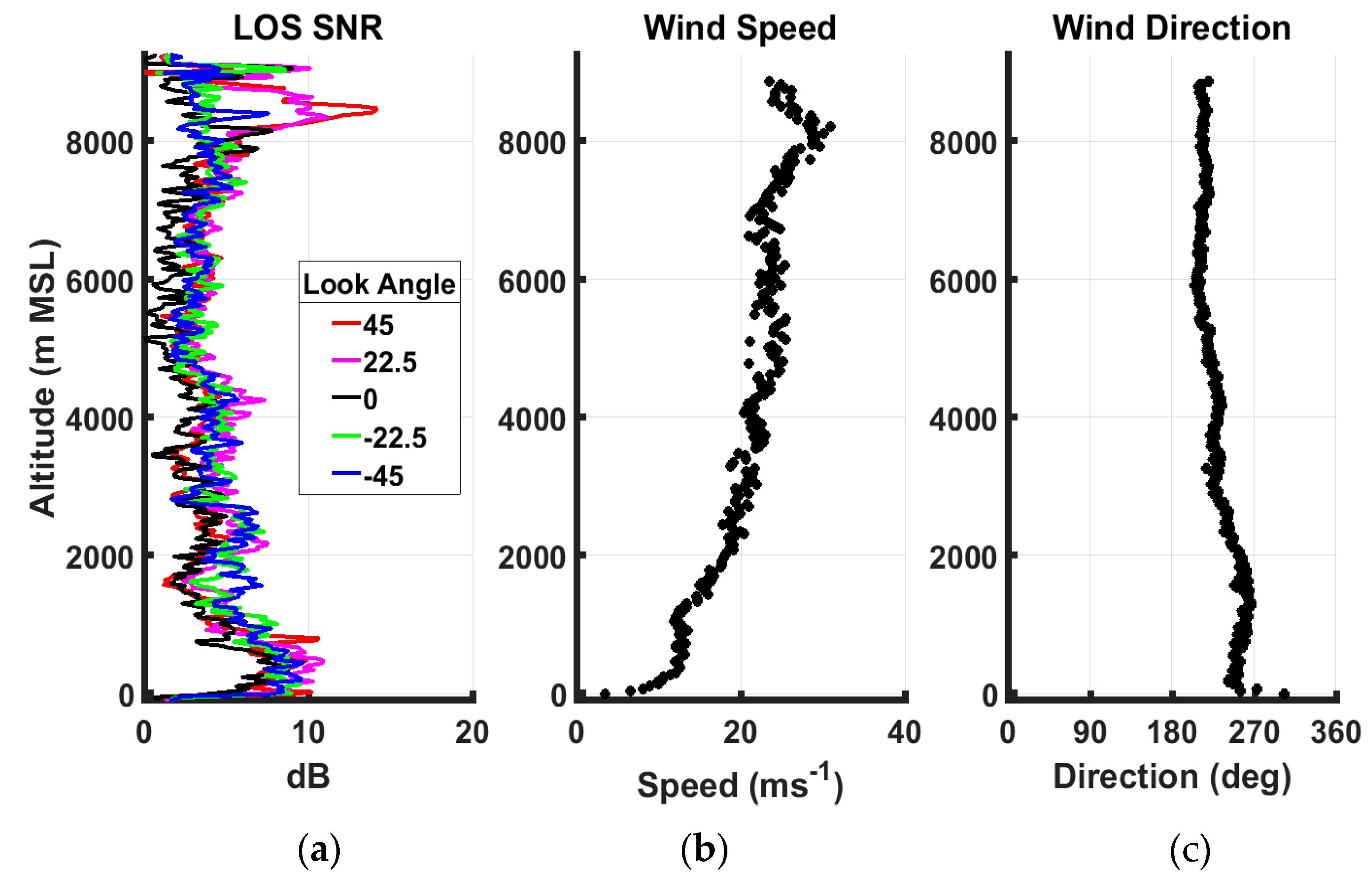
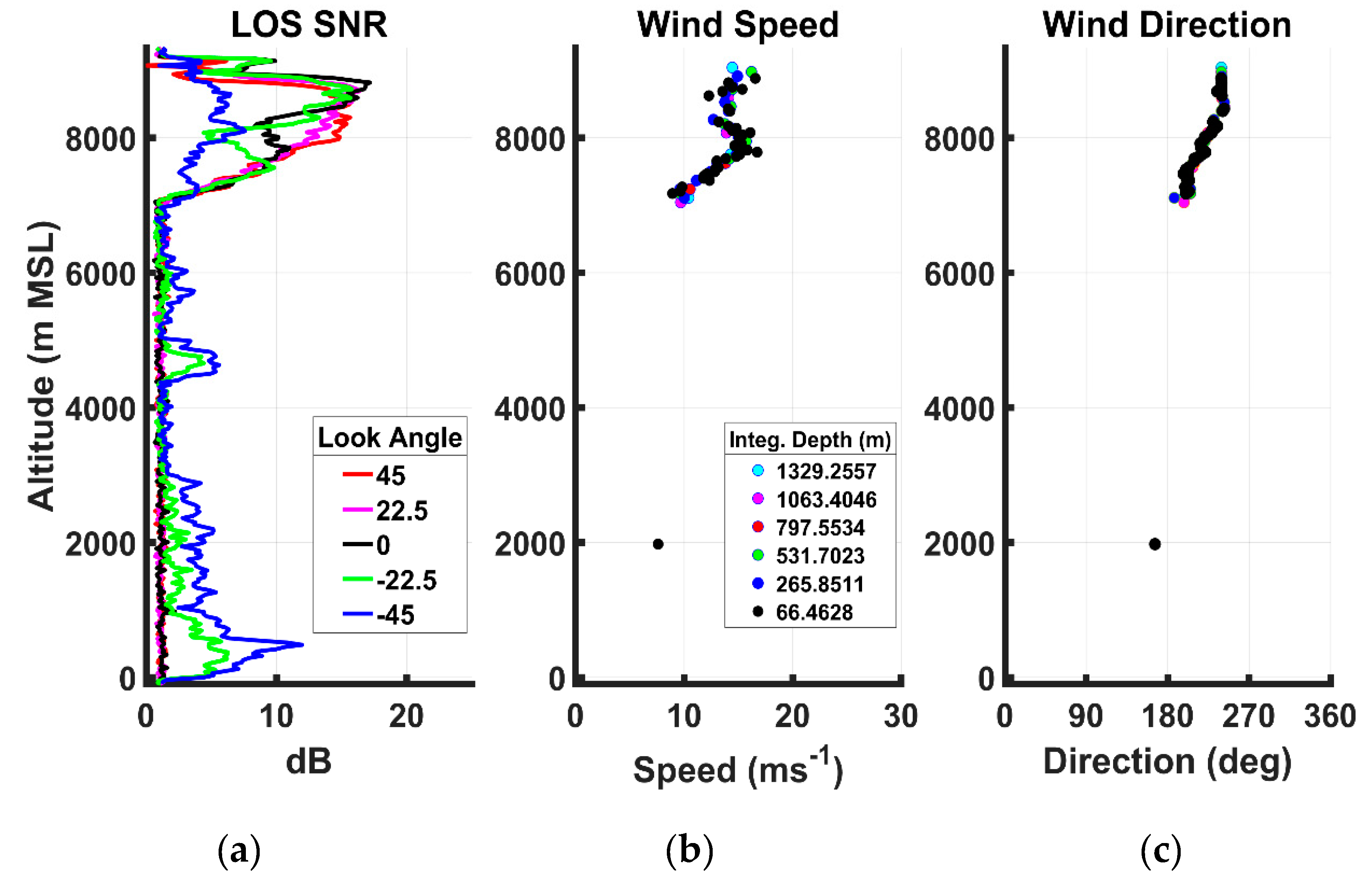
- Range gated LOS component of the 3-D wind vector illuminated along the range gate. The length of the range gate varies from ~30 m to 1000 m depending upon the strength of the backscattered signal measured as the SNR (in dB). The lidar system noise is determined from the range gates that are below the surface, i.e., from times when no reflected signal is being received.
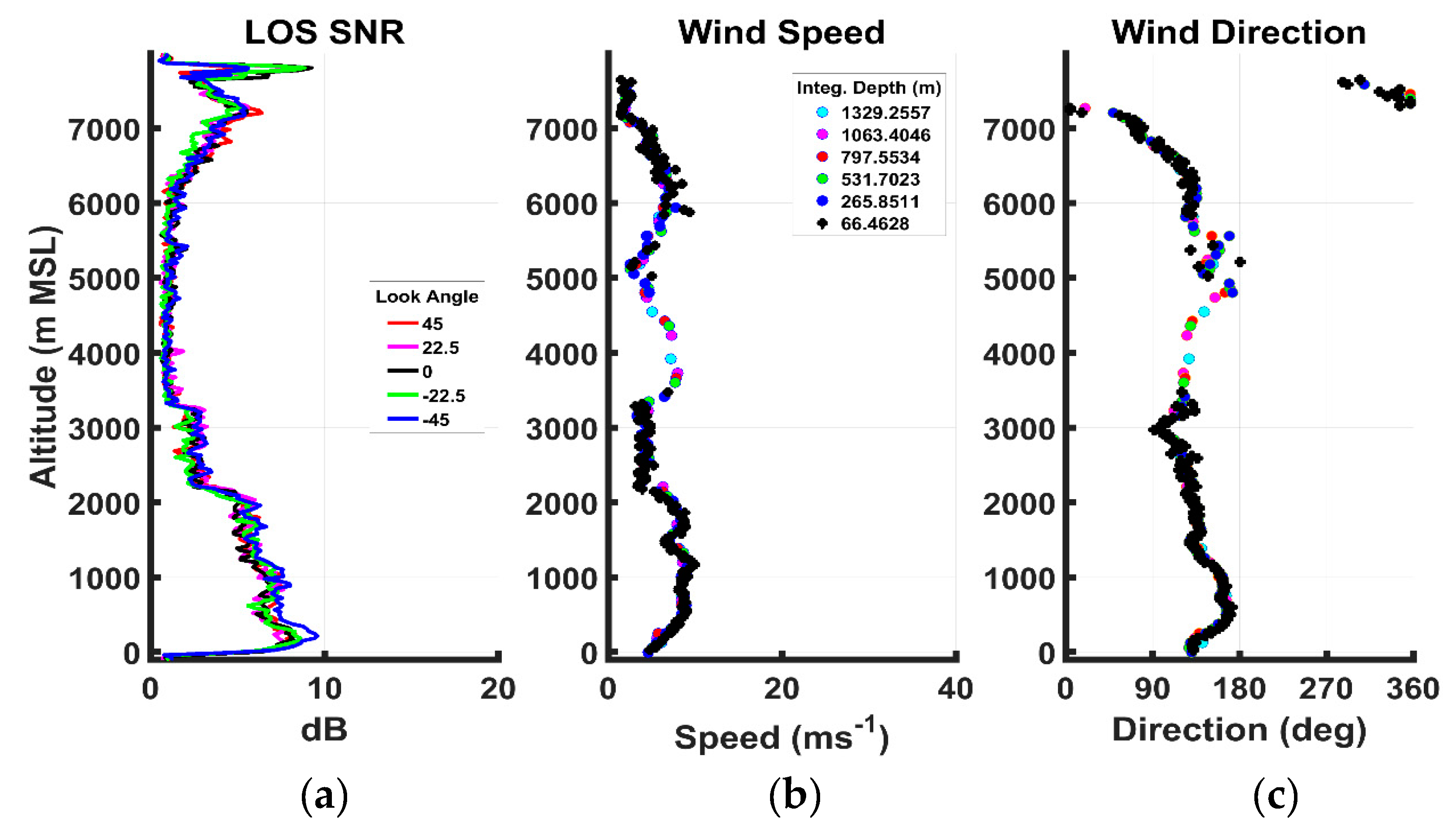
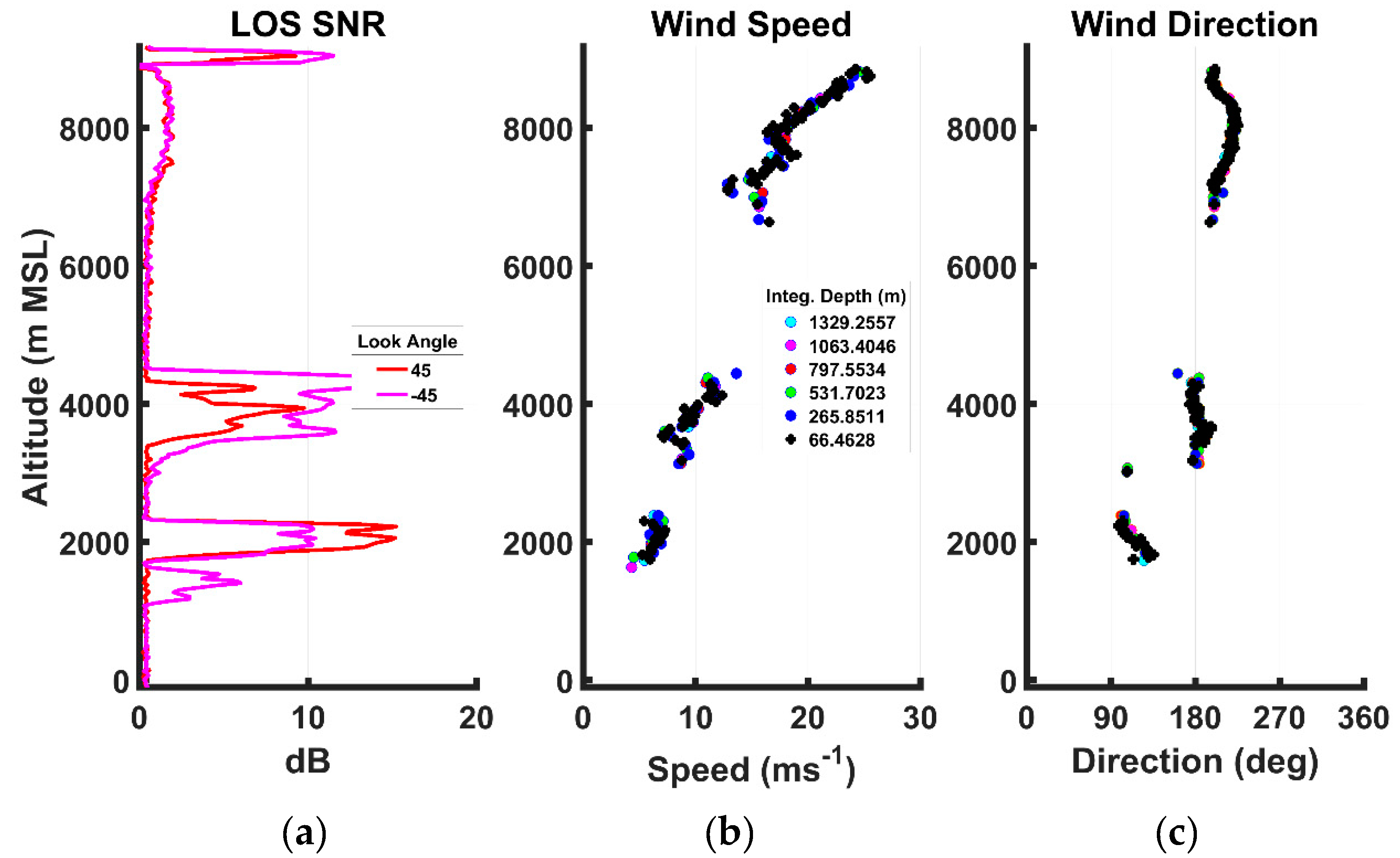
- Range gated LOS SNR determined from the power of the “information” peak in the frequency spectrum derived for each range gate.
3.2.1. LOS Adjustments
3.2.2. Wind Profile Retrieval and Products
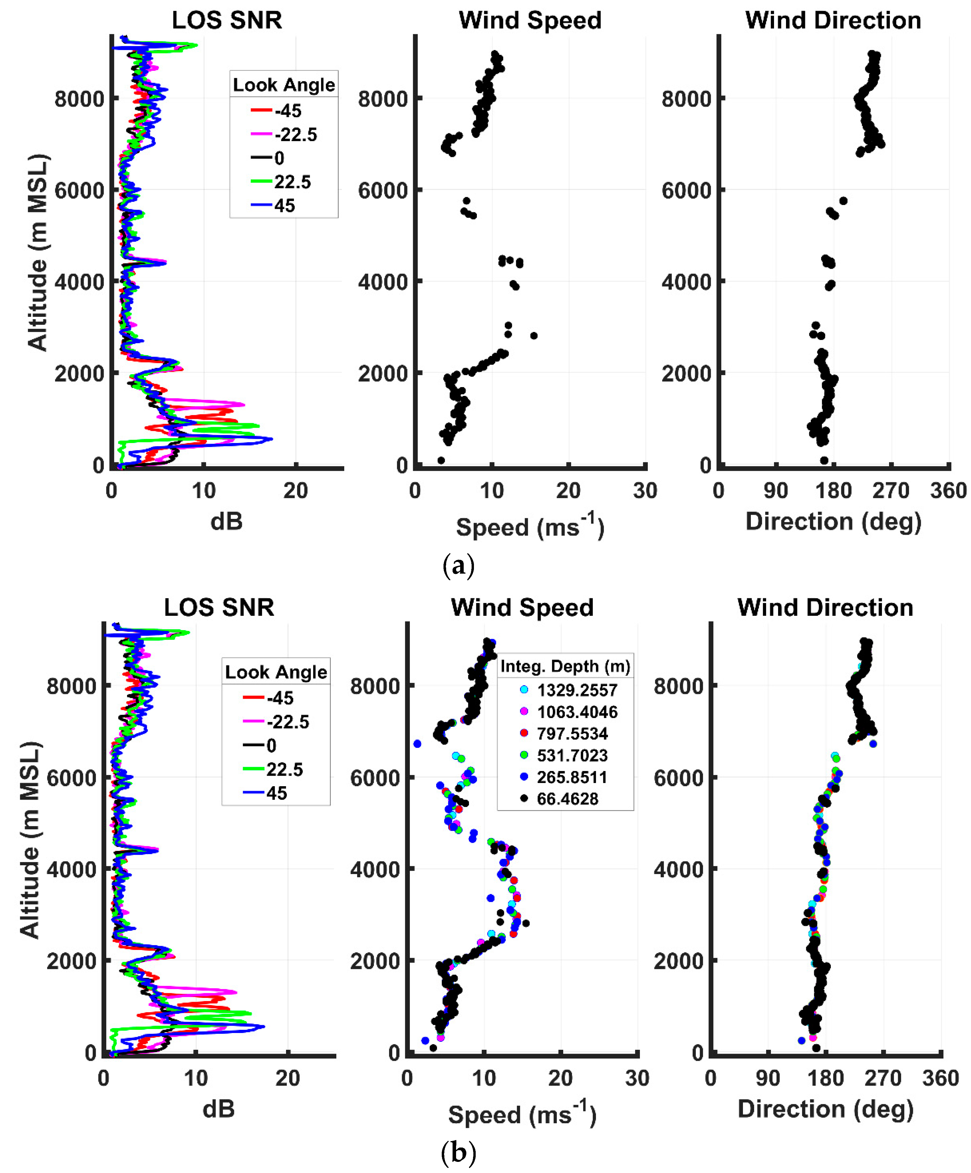
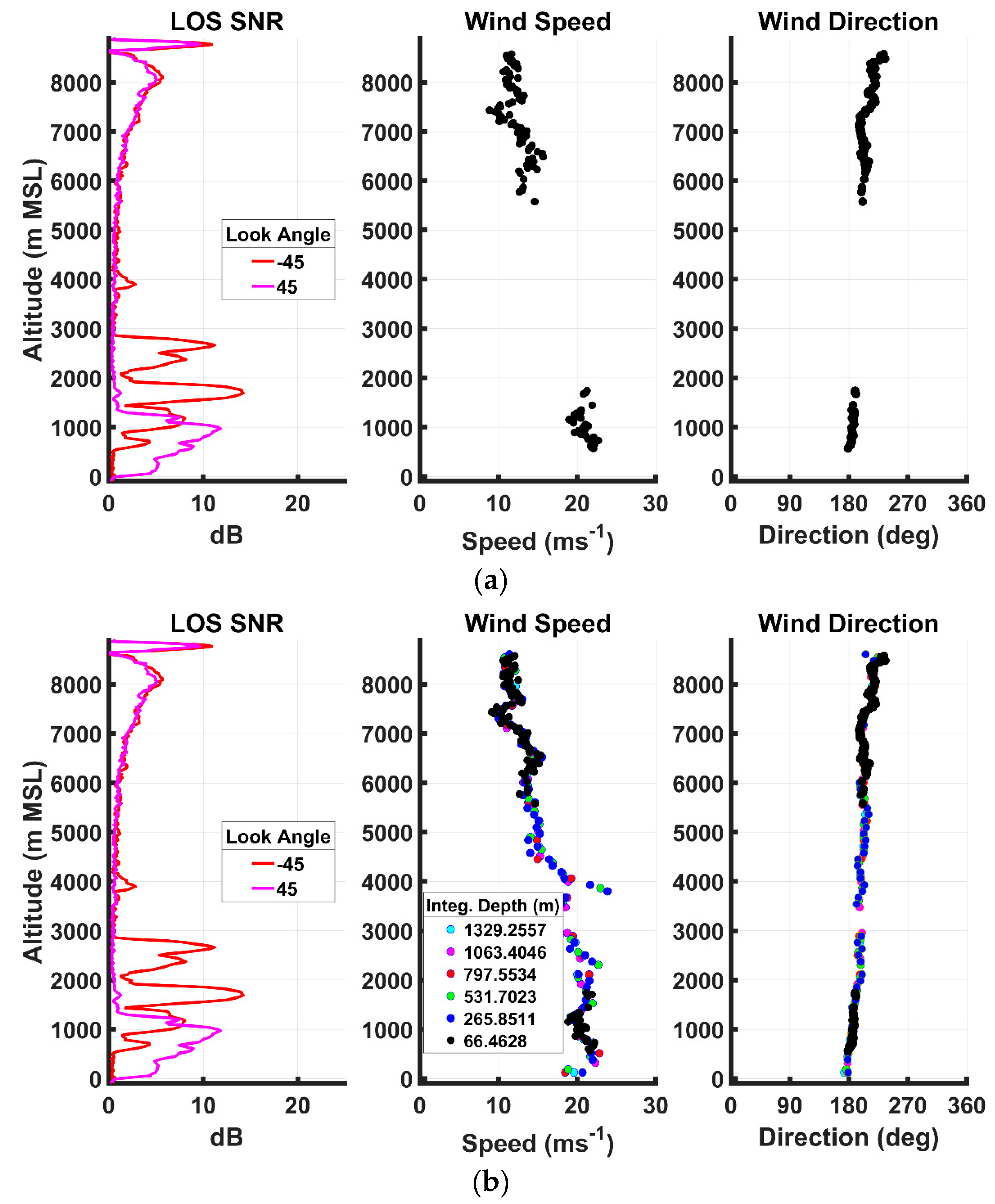
3.2.3. Adaptive Range Gate/Shot Integration for Wind Profiles
- Size of the “base” range gate.
- Maximum amount of LOS integrations appropriate for the atmospheric conditions.
- Integration lengths between the “base” range gate defined by 1. above and the maximum length of integration defined in 2. above.
- Threshold SNR for using a LOS integration in the LM wind vector solver.
- Threshold GOF for accepting wind profiles obtained from the LM wind vector solver.
4. Results
4.1. Evaluation of DAWN Performance
- The best performance in regard to providing full profiles was, as to be expected, during undisturbed days such as 27 May, 29 May and 23 June.
- Over 90% (4269 of 4585) of the processed DAWN base profiles on all missions provided needed measurements in the upper portions of the vertical column
- Despite the frequent attenuation of the DAWN signal by clouds in the convective environment, almost 50% of the processed DAWN base profiles provided useful measurements in the bottom 2 km, within or just above the MABL.
4.2. DAWN Data Comparisons
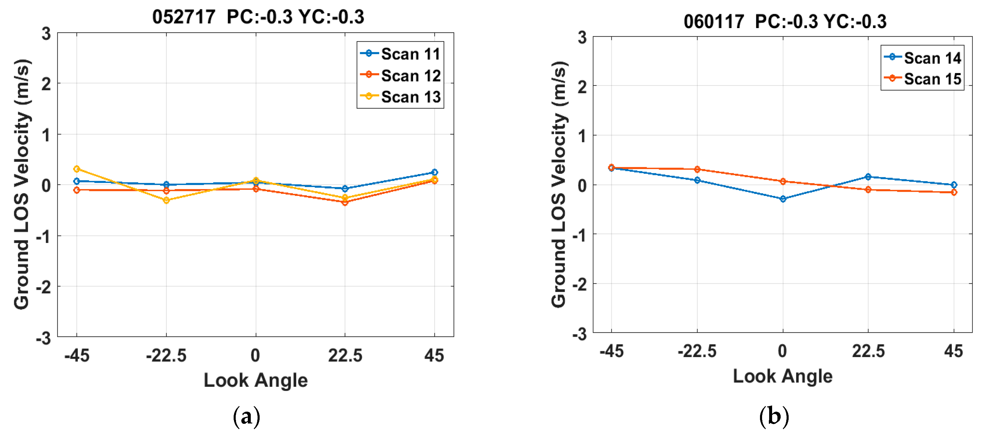
4.2.1. DAWN Measured Ground Speeds
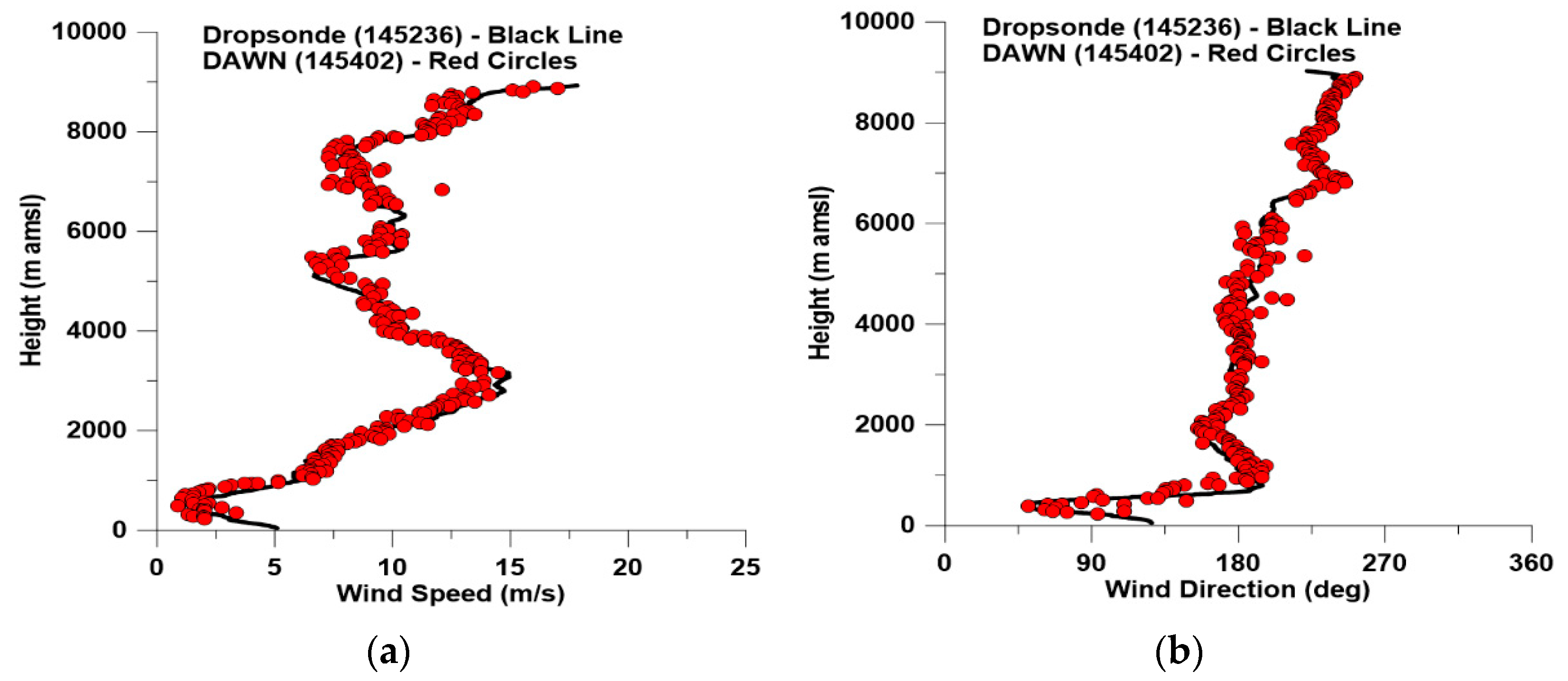
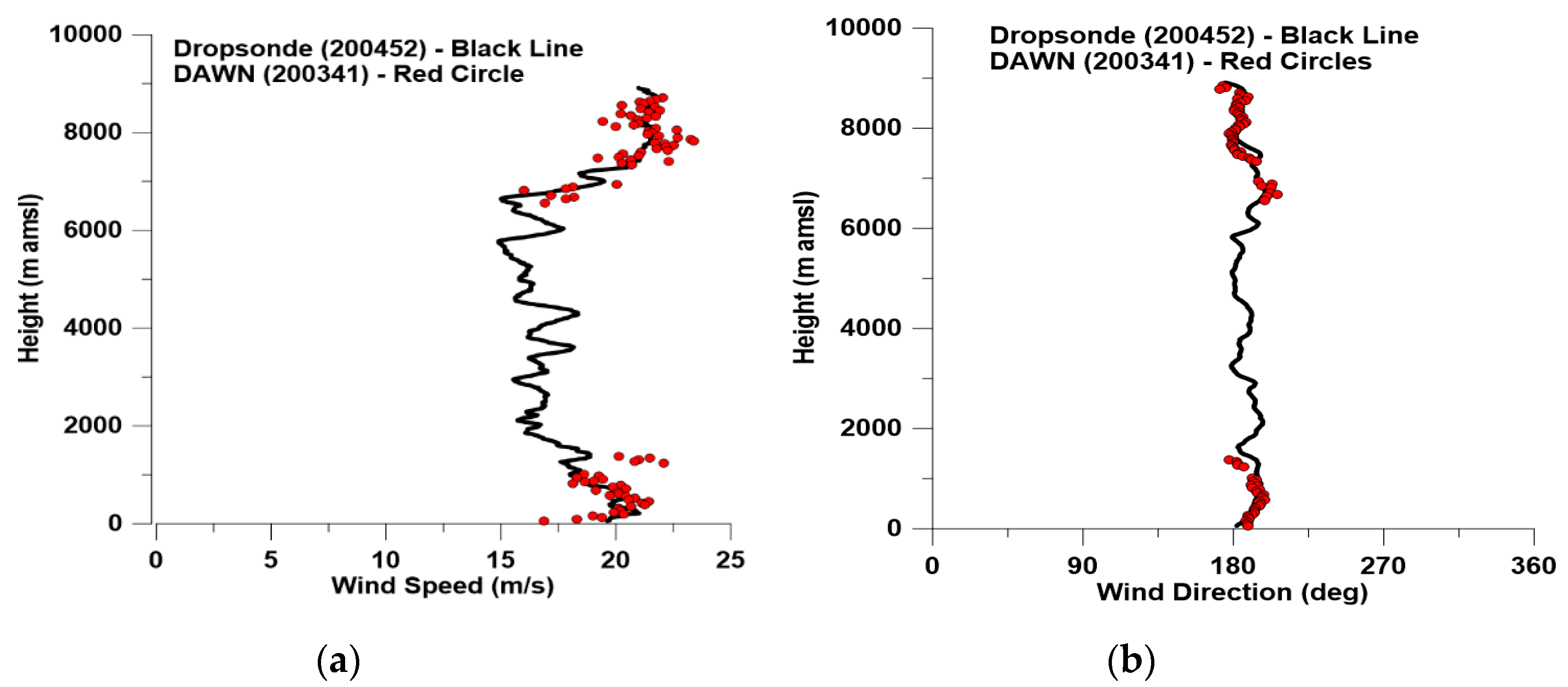
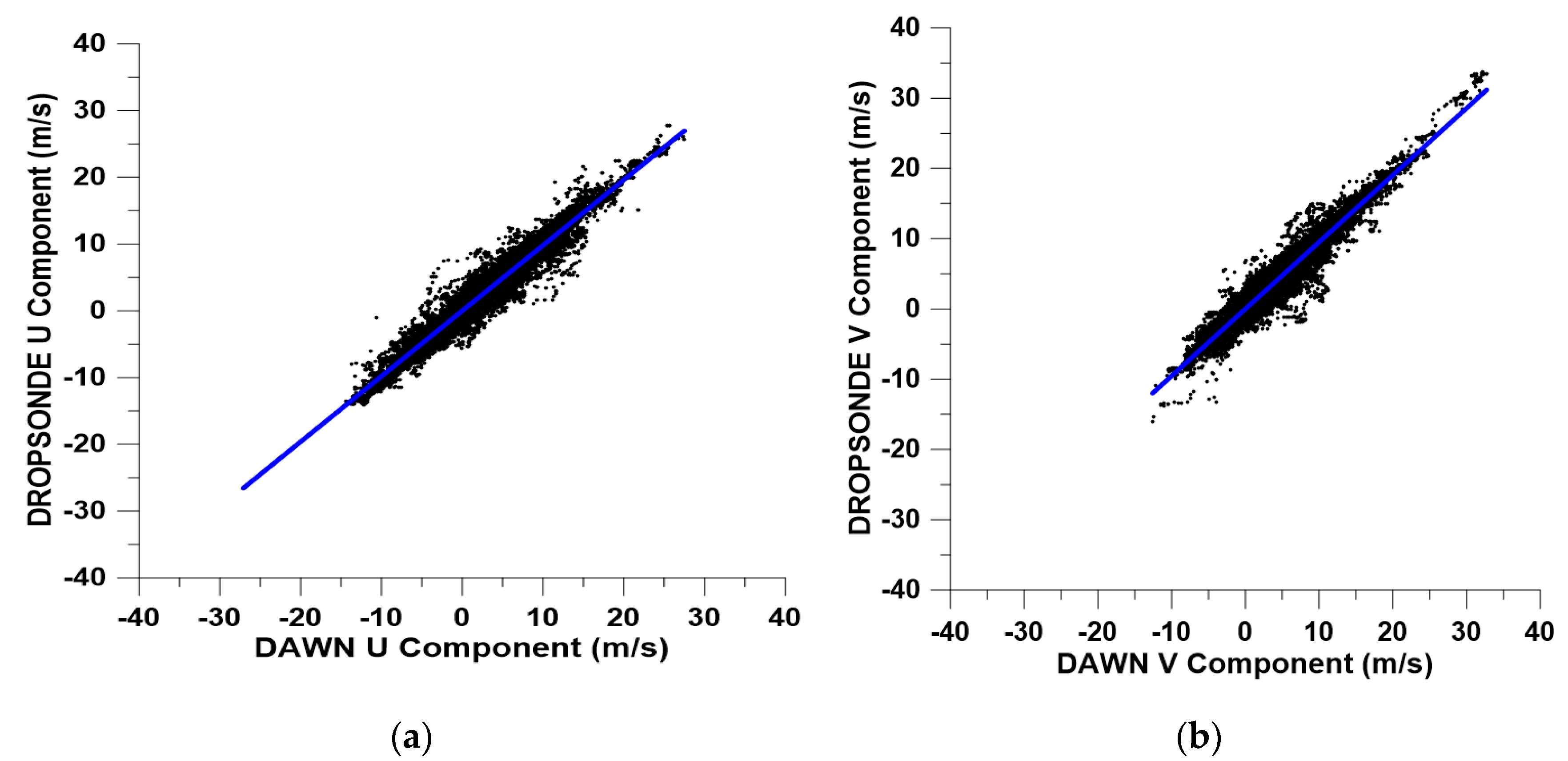
4.2.2. Vertical Profile Comparisons with Dropsondes
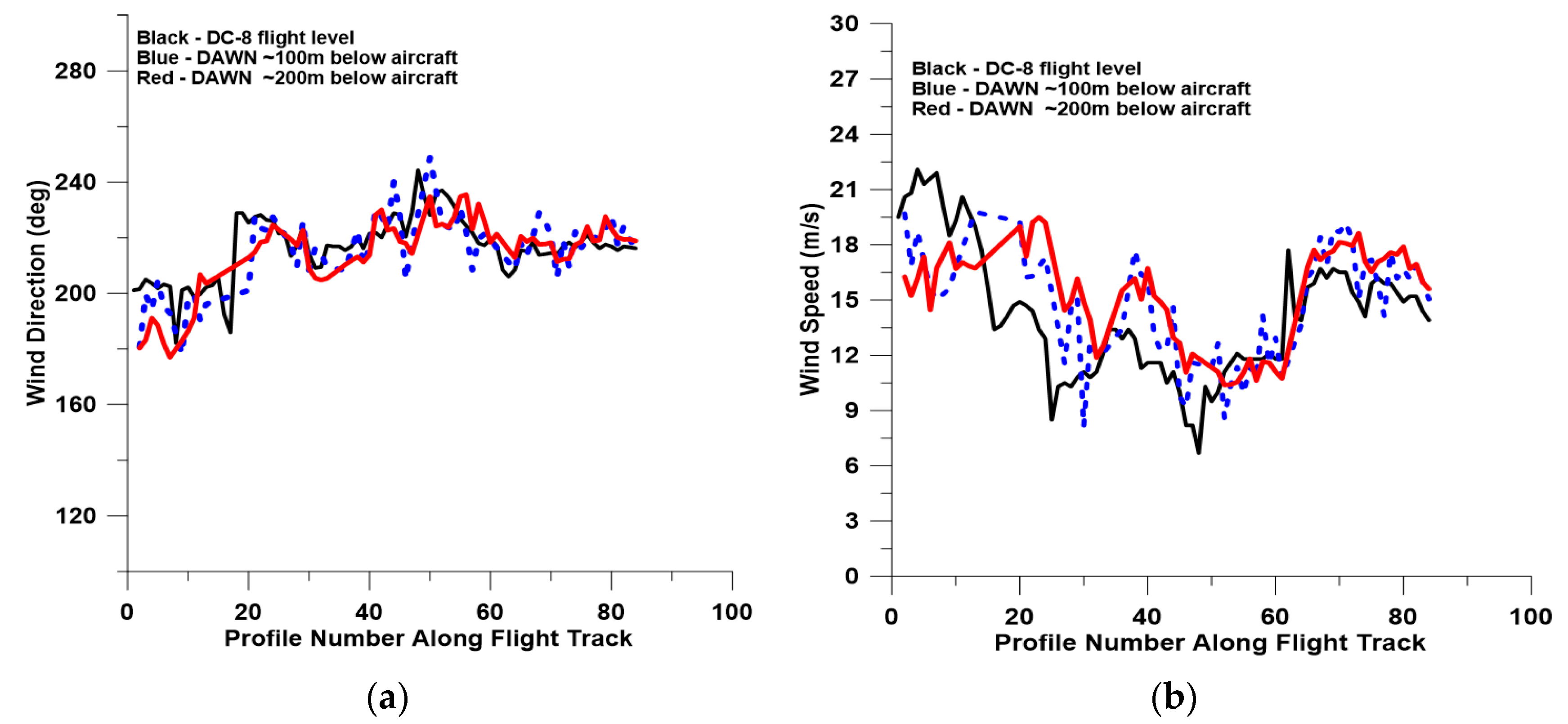
4.2.3. DAWN Comparisons with Flight Level Winds
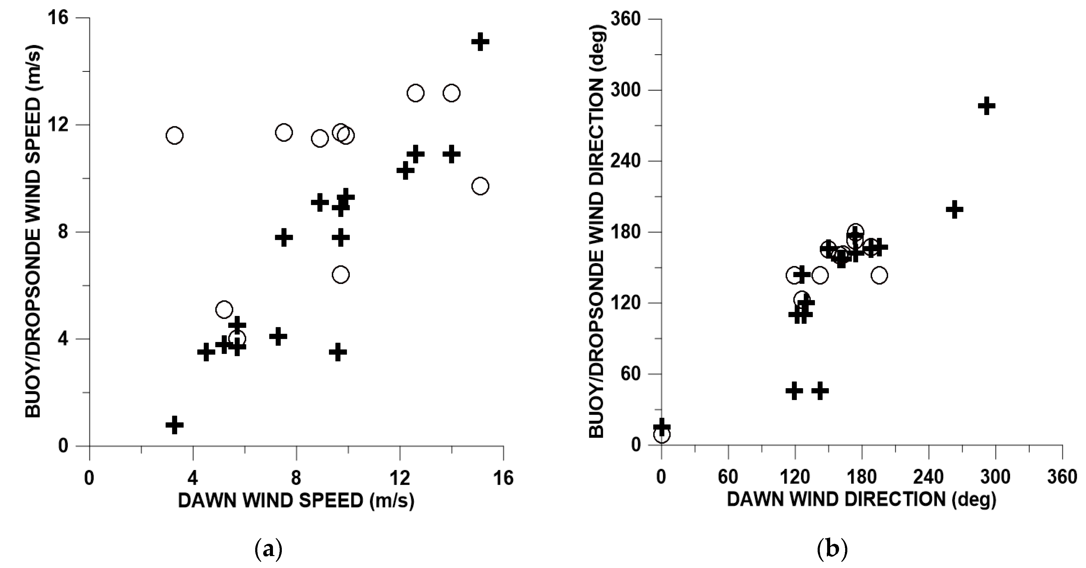
4.2.4. DAWN Near Surface Wind Comparisons with Dropsondes and Buoys
4.3. Case Studies
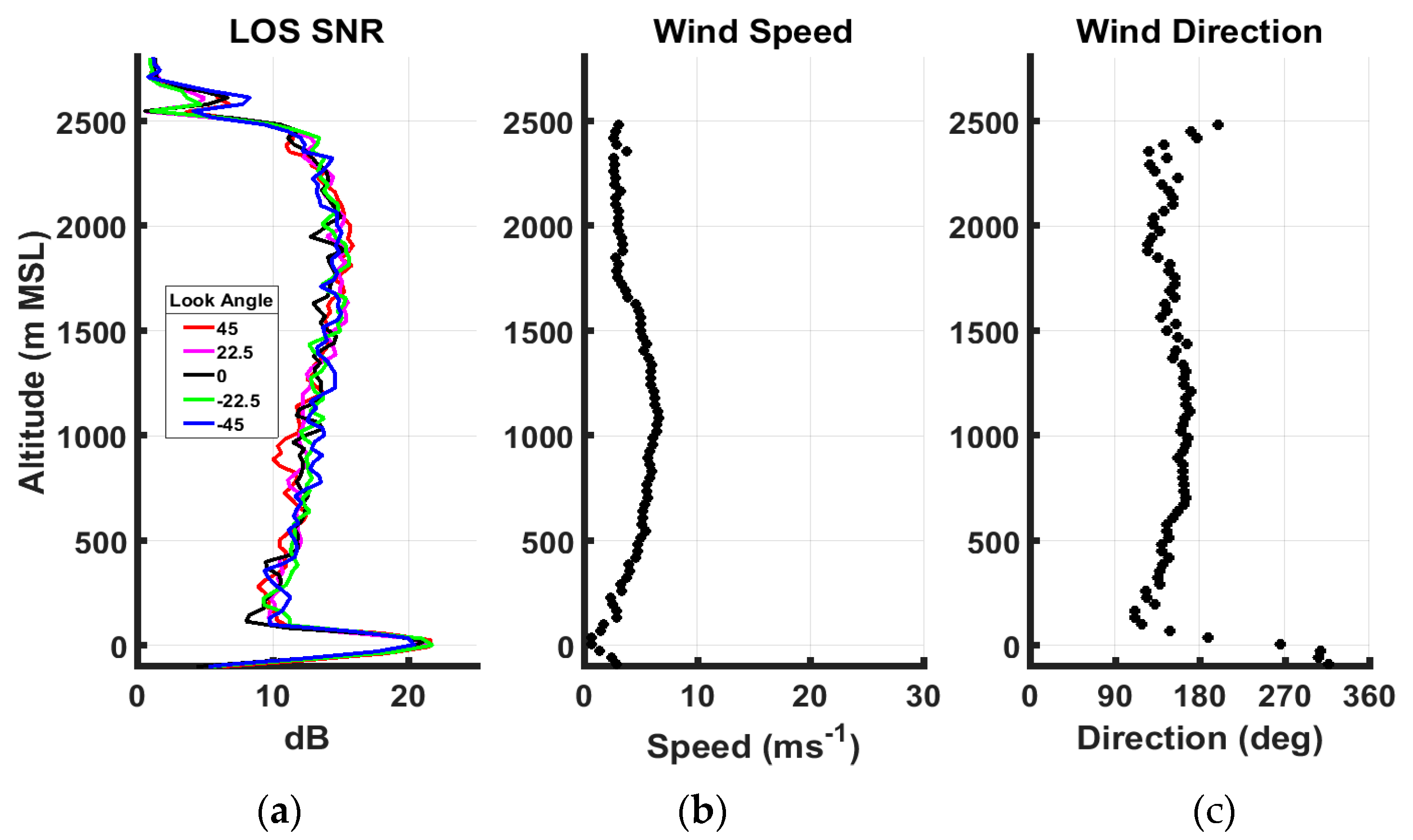
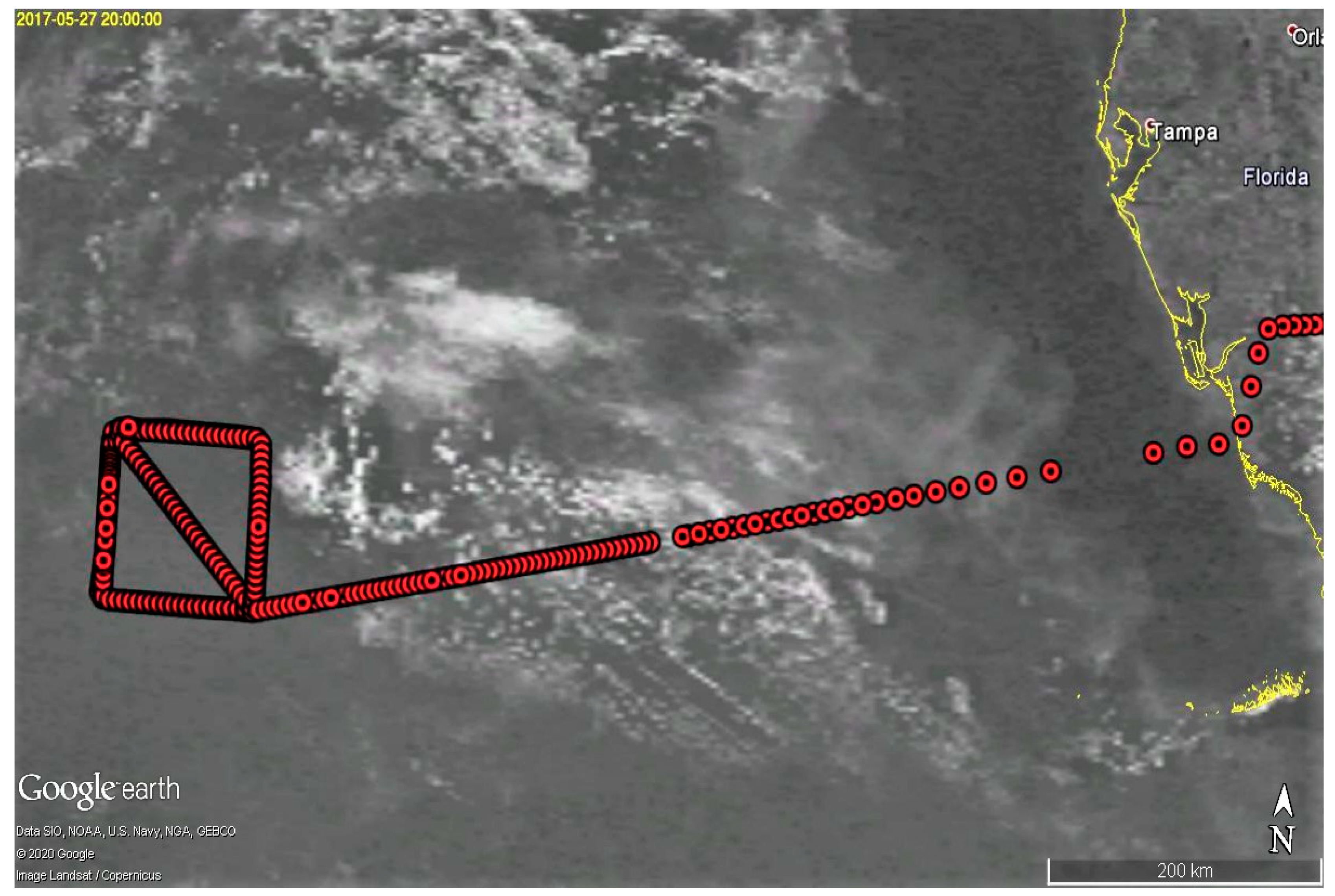
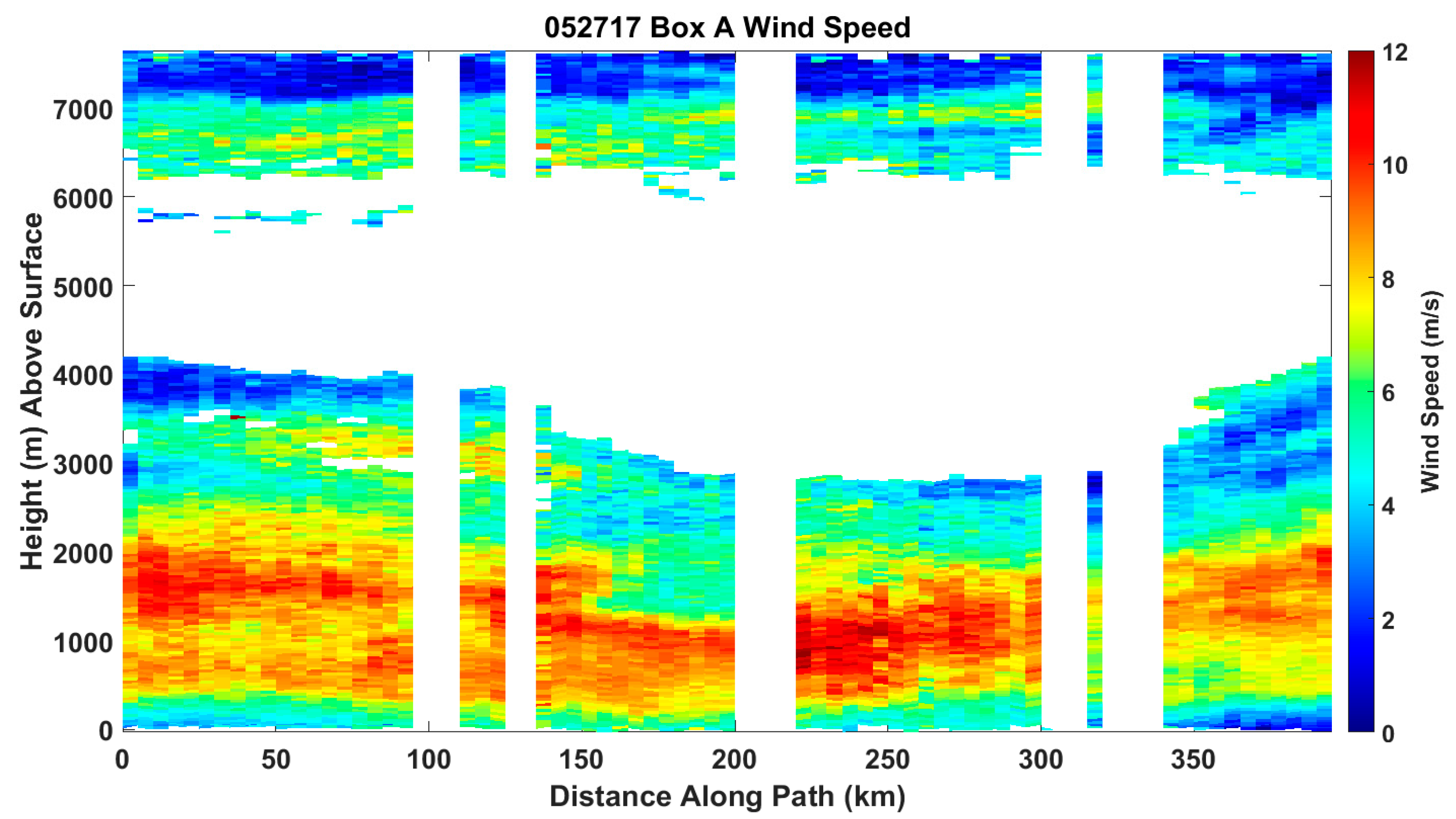
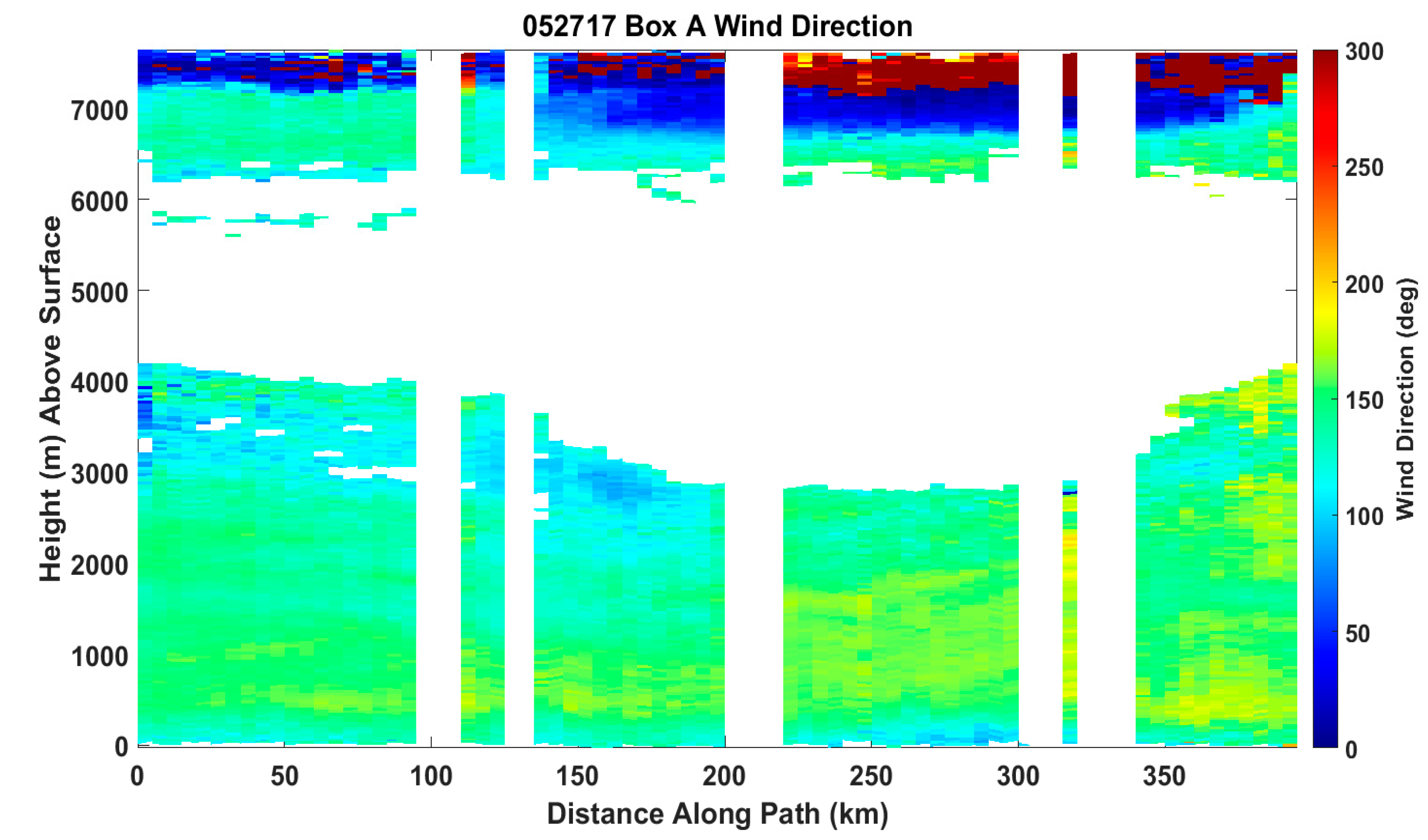
4.3.1. Undisturbed Conditions–27 May 2017
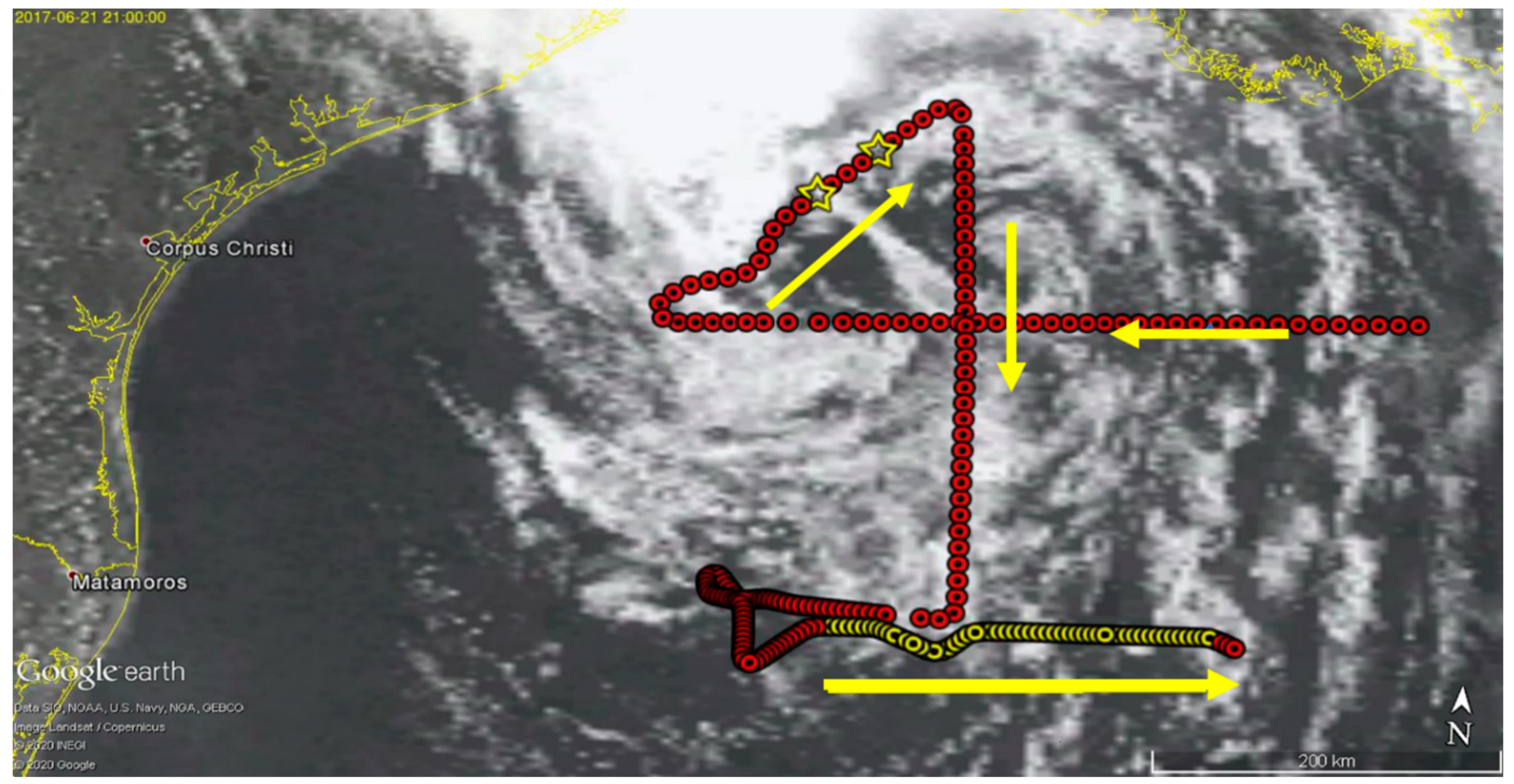
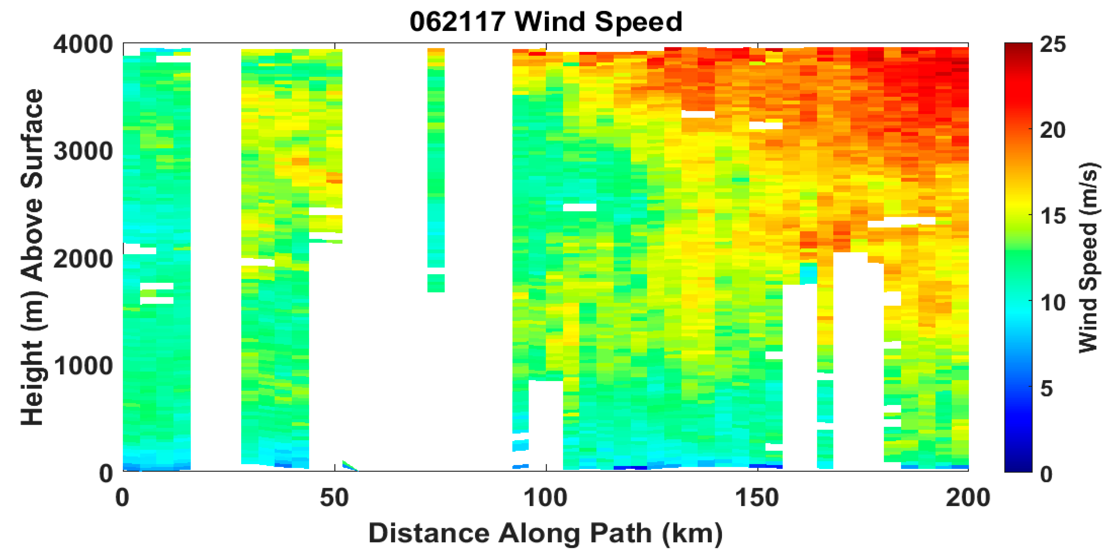
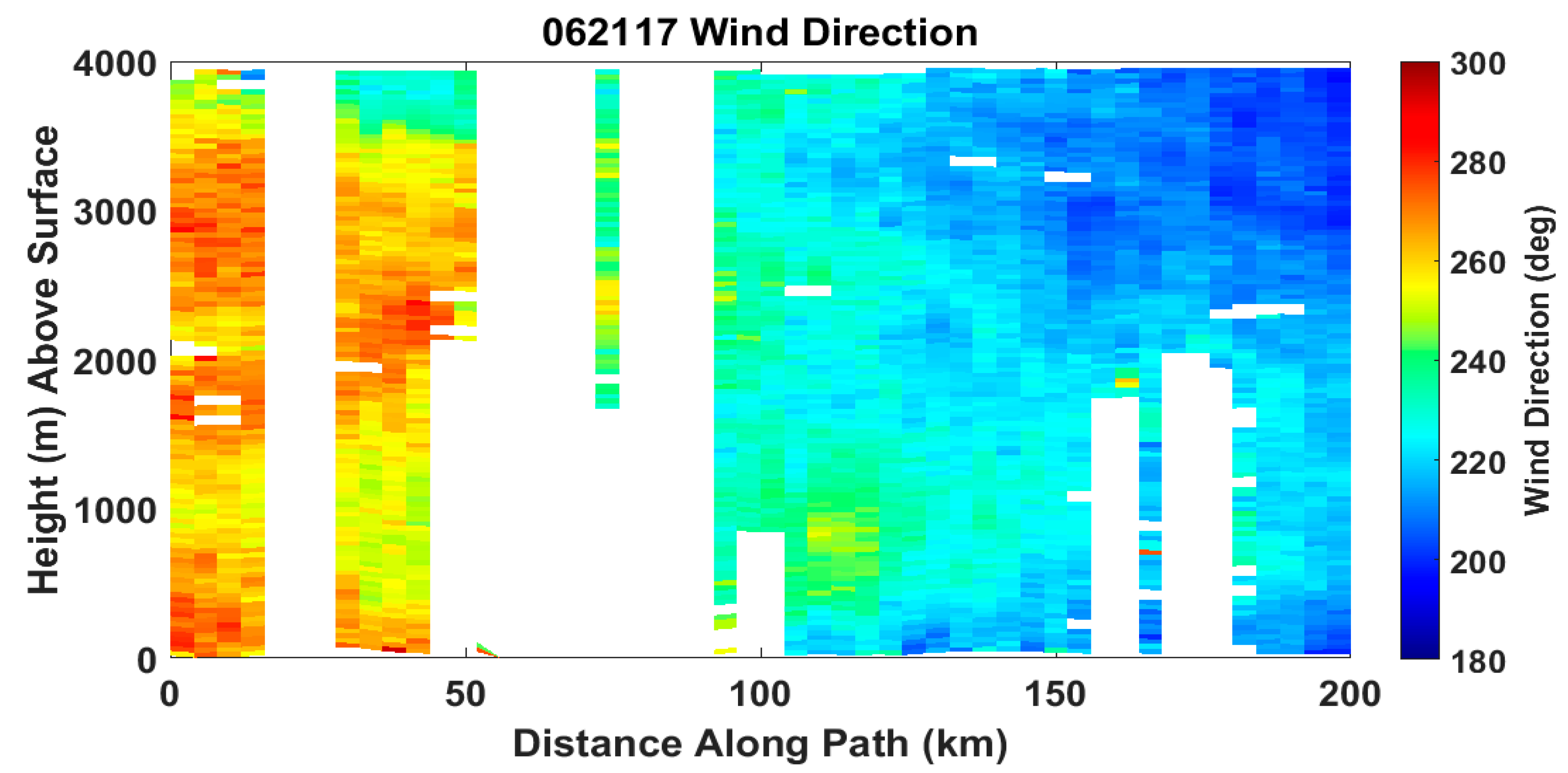
4.3.2. Investigation of Tropical Storm Cindy—21 June 2017
4.3.3. Organized Convection and Inflow—11 June 2017
5. Discussion
6. Conclusions
Author Contributions
Funding
Acknowledgments
Conflicts of Interest
Abbreviations
| ADWL | Airborne Doppler Wind Lidar |
| APR-2 | Airborne Second Generation Precipitation Radar |
| ASIA | Adaptive Sample Integration Algorithm |
| CPEX | Convective Processes Experiment |
| CPEX-AW | CPEX Aerosols and Winds |
| DAWN | Doppler Aerosol WiNd Lidar |
| FFT | Fast Fourier Transform |
| FOM | Figure Of Merit |
| FWHM | Full Width Half Max |
| GOES | Geostationary Operational Environmental Satellite |
| GOF | Goodness of Fit |
| GoM | Gulf of Mexico |
| GPS | Global Positioning System |
| GRIP | Genesis And Rapid Intensification Processes |
| HAMSR | High Altitude MMIC Sounding Radiometer |
| HDSS | High Definition Sounding System |
| HLOS | Horizontal Line-of-Sight |
| INS | Inertial Navigation System |
| JPL | Jet Propulsion Laboratory |
| LaRC | Langley Research Center |
| LM | Levenberg-Marquardt |
| LOS | Line-of-Sight |
| MABL | Marine Atmospheric Boundary Layer |
| MASC | Microwave Atmospheric Sounder for Cubesat |
| MTHP | Microwave Temperature and Humidity Profiler |
| NASA | National Aeronautics and Space Administration |
| NDBC | National Data Buoy Center |
| NOAA | National Oceanic and Atmospheric Administration |
| P3DWL | P-3 Doppler Wind Lidar |
| RMSD | Root Mean Square Difference |
| SNR | Signal to Noise Ratios |
| TODWL | Twin Otter Doppler Wind Lidar |
| TS | Tropical Storm |
| UWIN-CM | Unified Wave INterface-Coupled Model |
| XDD | eXpendable Digital Dropsonde |
| YES | Yankee Environmental Services |
References
- Kavaya, M.J.; Beyon, J.Y.; Koch, G.J.; Petros, M.; Petzar, P.J.; Singh, U.N.; Trieu, B.C.; Yu, J. The Doppler Aerosol Wind Lidar (DAWN) Airborne, Wind-Profiling, Coherent-Detection Lidar System: Overview, Flight Results, and Plans. J. Atmos. Ocean. Technol. 2014, 34, 826. [Google Scholar] [CrossRef]
- Black, P.; Harrison, L.; Beaubien, M.; Bluth, R.; Woods, R.; Penny, A.; Smith, R.W.; Doyle, J.D. High-definition Sounding System (HDSS) for atmospheric profiling. J. Atmos. Oceanic Technol. 2017, 34, 777–796. [Google Scholar] [CrossRef]
- Sadowy, G.A.; Berkun, A.C.; Chun, W.; Im, E.; Durden, S.L. Development of an advanced airborne precipitation radar. Microw. J. 2003, 46, 84–86. [Google Scholar]
- Brown, S.T.; Lambrigtsen, B.; Denning, R.F.; Gaier, T.; Kangaslahti, P.; Lim, B.H.; Tanabe, J.M.; Tanner, A.B. The High-Altitude MMIC Sounding Radiometer for the Global Hawk unmanned aerial vehicle: Instrument description and performance. IEEE Trans. Geosci. Remote Sens. 2011, 49, 3291–3301. [Google Scholar] [CrossRef]
- Lim, B.; Bendig, R.; Denning, R.; Pandian, P.; Read, W.; Tanner, A. The microwave temperature and humidity profiler instrument airborne shakeout performance. In Proceedings of the 2017 IEEE International Geoscience and Remote Sensing Symposium (IGARSS), Fort Worth, TX, USA, 23–28 July 2017; pp. 4530–4533. [Google Scholar]
- Tanelli, S.; Padmanabhan, S.; Peral, E.; Sy, O.; Durden, S.L.; Price, D.; Ortloff, B.; Parashare, C.; Turk, F.J.; Stachnick, R.; et al. Rain Cube and MASC in PECAN; Jet Propulsion Laboratory, California Institute of Technology: Pasadena, CA, USA, 2016. [Google Scholar]
- Trier, S.B. Convective Storms/Convective Initiation; Holton, J.R., Ed.; Encyclopedia Atmospheric Sciences Academic Press: London, UK, 2003; pp. 560–570. [Google Scholar]
- Pu, Z.; Zhang, L.; Emmitt, G.D. Impact of airborne Doppler wind lidar profiles on numerical simulations of a tropical cyclone. Geophy. Res. Lett. 2010, 37. [Google Scholar] [CrossRef]
- Waliser, D.E.; Moncrieff, M.W.; Burridge, D. The “Year” of tropical convective (May 2008–April 2010): Climate variability and weather highlights. Bull. Amer. Meteor. Soc. 2012, 93, 1189–1218. [Google Scholar] [CrossRef]
- Cui, Z.; Pu, Z.; Emmitt, G.D.; Greco, S. The Impact of Airborne Doppler Aerosol WiNd lidar (DAWN) Wind Profiles on Numerical Simulations of Tropical Convective Systems during the NASA Convective Processes Experiment (CPEX). J. Atmos. Oceanic Technol. 2020, 37, 705–722. [Google Scholar] [CrossRef]
- Turk, J.; Hristova-Veleva, S.M.; Durden, S.; Tanelli, S.; Sy, O.; Emmitt, D.; Greco, S.; Zhang, S. Joint Analysis of Convective Structure from the APR-2 Precipitation Radar and the DAWN Doppler Wind Lidar during the 2017 Convective Processes Experiment (CPEX). Atmos. Meas. Tech. 2020, in press. [Google Scholar] [CrossRef]
- Yu, J.; Trieu, B.C.; Modlin, E.A.; Singh, U.N.; Kavaya, M.J.; Chen, S.; Bai, Y.; Petzar, P.J.; Petros, M. 1 J/pulse Q-switched 2-micron solid-state laser. Opt. Letters. 2006, 31, 462. [Google Scholar] [CrossRef] [PubMed]
- Singh, U.N.; Walsh, B.M.; Yu, J.; Petros, M.; Kavaya, M.J.; Refaat, T.F.; Barnes, N.P. 20 years of Tm,Ho:YLF and LuLF Laser Development for Global Winds Measurements. Opt. Mater. Express. 2015, 5, 827. [Google Scholar] [CrossRef]
- Greco, S.; Emmitt, G.D. Investigation of flows within complex terrain and along coastlines using an airborne Doppler wind lidar: Observations and model comparisons. In Proceedings of the Sixth Conference on Coastal Atmospheric and Oceanic Prediction and Processes, Annual American Meeting Society Conference, San Diego, CA, USA, 25–28 January 2005. [Google Scholar]
- Bucci, L.R.; O’Handley, C.; Emmitt, G.D.; Zhang, J.A.; Ryan, K.; Atlas, R. Validation of an Airborne Doppler Wind Lidar in Tropical Cyclones. Sensors 2018, 18, 4288. [Google Scholar] [CrossRef] [PubMed]
- Greco, S.; Emmitt, G.D.; Wood, S.A. Recent Airborne Doppler Wind Lidar Investigations of Lower Troposphere Circulations from the Tropics to the Poles. In Proceedings of the American Meteorology Society 97th Annual Meeting, Observation Symposium Poster Session, Seattle, WA, USA, 22–26 January 2017. [Google Scholar]
- Greco, S.; Emmitt, G.D.; Kavaya, M.; Kakar, R.; Cassano, J.J.; Hines, K. Airborne Doppler Wind Lidar Missions in the Arctic: Low Level Observations and Comparison with Models and other Observing Platforms. In Proceedings of the American Meteorology Society 96th Annual Meeting, 20th Conference on Integrated Observing and Assimilation Systems for the Atmosphere, Oceans, and Land Surface (IOAS-AOLS), New Orleans, LA, USA, 10–14 January 2016. [Google Scholar]
- DuVivier, A.K.; Cassano, J.J.; Greco, S.; Emmitt, G.D. A case study of observed and modeled barrier flow in the Denmark Strait in May 2015. Mon. Weather Rev. 2017, 145, 2385–2404. [Google Scholar] [CrossRef]
- Emmitt, G.D.; Godwin, K.S.; Greco, S.; Wood, S.A. The 2014–2015 Polar Winds DAWN Airborne Campaigns; Instrument Performance, Data Collection and Advanced data Processing Algorithm Development. In Proceedings of the American Meteorology Society 97th Annual Meeting, 8th Symposium on Lidar Atmospheric Applications, Seattle, WA, USA, 16–28 January 2017. [Google Scholar]
- Liu, Z.; Kavaya, M.J.; Bedka, K.M. Coherent Doppler Wind Lidar Data Processing Software and Wind Retrieval from the Aeolus Cal/Val Field Campaign. In Proceedings of the ADM-Aeolus CAL/VAL Rehearsal, Météo-France, Toulouse, France, 28–30 March 2019; p. A12A-07. [Google Scholar]
- Koch, G.; Beyon, J.Y.; Cowen, L.J.; Kavaya, M.J.; Grant, M.S. Three-dimensional wind profiling of offshore wind energy areas with airborne Doppler lidar. J. Appl. Remote Sens. 2014, 8, 083662. [Google Scholar]
- Koch, G.; Beyon, J.Y.; Modlin, E.A.; Petzar, P.J.; Woll, S.; Petros, M.; Yu, J.; Kavaya, M.J. Side-scan Doppler lidar for offshore wind energy applications. J. Appl. Remote Sens. 2012, 6, 063562. [Google Scholar] [CrossRef]
- Creasey, R.L.; Elsberry, R.L. Tropical cyclone center positions from sequences of HDSS sondes deployed along high-altitude overpasses. Weather Forecast. 2017, 32, 317–325. [Google Scholar] [CrossRef]
- Nelson, T.C.; Harrison, L.; Corbosiero, K.L. Examination of the Expendable Digital Dropsonde–Derived Vertical Velocities from the Tropical Cyclone Intensity (TCI) Experiment. Mon. Weather Rev. 2019, 147, 2367–2386. [Google Scholar] [CrossRef]
- Liu, W.T.; Katsaros, K.B.; Businger, J.A. Bulk Parameterizations of Air-Sea Exchanges of Heat and Water Vapor Including Molecular Constraints at the Interface. J. Atmos. Sci. 1979, 36, 1722–1735. [Google Scholar] [CrossRef]
- LeMone, M.A.; Zipser, E.J.; Trier, S.B. The role of environmental shear and thermodynamic conditions in determining the structure and evolution of mesoscale convective systems during TOGA COARE. J. Atmos. Sci. 1998, 55, 3493–3518. [Google Scholar] [CrossRef]


| Mission | Location Focus | Vertical Extent | DAWN Hor. Res. | Number of XDD | Atmospheric Environment |
|---|---|---|---|---|---|
| 27 May | GoM | 7–8 km | 3–7 km | 9 (9) | undisturbed |
| 29 May | Caribbean Sea | 8–9 km | 5–7 km | 15 (13) | scattered. shallow convection |
| 31 May | east of Bahamas | 9–10 km | 10–15 km | 16 (13) | scattered/isolated convection |
| 1 June | eastern GoM | 12 km | 7–15 km | 21 (13) | organized convection |
| 2 June | GoM | 12 km | 5–10 km | 19 (17) | convection |
| 6 June | eastern GoM | 9 km | 7–10 km | 7 (6) | undisturbed west; convection east |
| 10 June | east of Bahamas | 9–10 km | 4–6 km | 26 (14) | targeted mesoscale cluster |
| 11 June | Central GoM | 8–10 km | 7–10 km | 28 (14) | organized convection and inflow |
| 15 June | Caribbean Sea | 10 km | 4–7 km | 9 (4) | active convection |
| 16 June | Caribbean Sea | 10 km | 10–15 km | 28 (12) | convection |
| 17 June | Caribbean Sea | 9–12 km | 7–10 km | 20 (NA) | convection |
| 19 June | GoM | 12 km | 3–15 km; | 19 (8) | convection; precursor TS Cindy |
| 20 June | central GoM | 10–12 km | 9–12 km | 16 (12) | TS Cindy; convective and inflow |
| 21 June | Northern GoM | 4–12 km | 9–12 km | 30 (22) | TS Cindy (southern inflow) |
| 23 June | east of Bahamas | 7 km | 10–20 km; | 7 (6) | undisturbed/isolated convection |
| 24 June | Caribbean Sea | 10–12 km | 10–20 km; | 9 (NA) | undisturbed and convection |
| Attribute | Value |
|---|---|
| Airplanes flown | DC-8 and UC-12B |
| Solid-state laser crystal and wavelength | Ho:Tm:LuLiF, 2.053472 microns |
| Laser pulse energy, rate, and FWHM duration | 250 mJ, 10 Hz, 180 ns |
| Receiver telescope diameter | 15 cm; the transmitted laser beam is aligned for the optimum (coherent detection, diffuse target) e−2 intensity diameter of 12 cm |
| Scan pattern | Step-stare, 30-deg half angle conical, centered on nadir |
| Number of LOS/azimuth angles | SelecTable 1, 2, 5, 8 or 12 |
| Number of laser shots at each LOS | Selectable, typically 10–20 (1–2 s) |
| Optical detection | Dual-balanced coherent (heterodyne), InGaAs |
| Laser pointing knowledge | Dedicated INS/GPS on lidar supplemented by ground returns |
| Parameter | DAWN | TODWL | P3DWL | Comments |
|---|---|---|---|---|
| Wavelength (microns) | 2.05 | 2.05 | 1.67 | |
| Energy per pulse (mJ) | 100 | 1 | 2 | |
| Pulse rate(Hz) | 10 | 500 | 500 | |
| Pulse length(m) | ~30 | 90 | 90 | Range resolution |
| Telescope diameter(m) | 0.15 | 0.10 | 0.10 | |
| Detection type | Coherent | Coherent | Coherent | 0.5 m/s LOS precision |
| Weight(kg) | 450 | 300 | 275 | Approximate weights |
| Power(watts) | 3250 | 700 | 550 | Approximate power |
| FOM ** | 1.14 | 0.02 | 0.05 |
| Pointing/Accuracy | DC-8 at 10 km FL | Twin Otter at 1 km FL | Comments | ||
|---|---|---|---|---|---|
| HLOS Vel | Height | HLOS Vel | Height | Height Errors for Layer Just above the Surface | |
| Pitch Error (deg) | 0.03 | 0.1 | 0.13 | 1.0 | |
| Roll Error (deg) | 0.14 | 0.6 | 1.0 | 6.0 | Reference roll is wings level |
| Yaw Error (deg) | 0.02 | 0.0 | 0.12 | 0.0 | Ground track heading reporting error |
| LOS Wind Measurement Precision | ~1 m/s; Bias < 0.25 m/s |
|---|---|
| u, v, w measurement precision | <~1.5 m/s; bias < 0.2 m/s |
| Data product vertical resolution | 30–150 m., selectable in post-processing |
| Horizontal resolution of each LOS wind profile | 500 m typical (variable with # shots) |
| Horizontal resolution of vertical profile of horizontal wind | 3–20 km (variable with # LOS, # shots, aircraft ground speed) |
| Mission | Profiles Attempted | Not Processed (Turn/Climb) | Successful Profiles | Full Profiles | Top 2 km Below DC8 | Lower 2 km |
|---|---|---|---|---|---|---|
| 27 May | 320 | 39 | 281 | 155 | 267 | 277 |
| 29 May | 412 | 77 | 335 | 49 | 329 | 294 |
| 31 May | 232 | 35 | 197 | 2 | 185 | 180 |
| 1 June | 372 | 124 | 248 | 4 | 241 | 41 |
| 2 June | 583 | 58 | 525 | 0 | 508 | 52 |
| 6 June | 266 | 108 | 158 | 71 | 141 | 66 |
| 10 June | 540 | 138 | 402 | 36 | 376 | 174 |
| 11 June | 415 | 97 | 318 | 51 | 295 | 88 |
| 15 June | 422 | 100 | 322 | 15 | 291 | 86 |
| 16 Jun | 119 | 23 | 96 | 7 | 94 | 55 |
| 17 June | 407 | 162 | 245 | 42 | 159 | 57 |
| 19 June | 354 | 58 | 296 | 2 | 258 | 10 |
| 20 June | 196 | 39 | 157 | 2 | 154 | 71 |
| 21 June 0–4 km | 430 210 | 113 76 | 317 134 | 105 * 105 | 314 * 133 | 200 105 |
| 23 June | 747 | 179 | 568 | 119 | 549 | 498 |
| 24 June | 205 | 85 | 120 | 4 | 108 | 75 |
| Total | 6020 | 1435 | 4585 (76%) | 664 | 4269 | 2224 (48%) |
| # of Comps | Mean ∆z (m) | Mean ∆v (bias) | RMSD ∆v | R2 Coefficient Y = B × X + A | B | A | |
|---|---|---|---|---|---|---|---|
| Sfc-3 km | 4808 | 2.52 | 0.17 | 1.29 | 0.922 | 0.97 | 0.07 |
| 3–6 km | 1866 | 2.89 | 0.21 | 1.67 | 0.893 | 0.91 | 0.30 |
| 6–9 km | 6012 | 3.35 | 0.28 | 1.72 | 0.918 | 0.93 | 0.66 |
| 9–12 km | 3521 | 3.62 | 0.10 | 1.78 | 0.922 | 0.97 | 0.07 |
| ALL | 16,207 | 3.11 | 0.19 | 1.61 | 0.923 | 0.95 | 0.05 |
| # of Comps | Mean ∆z (m) | Mean ∆u (bias) | RMSD ∆u | R2 Coefficient Y = B × X + A | B | A | |
|---|---|---|---|---|---|---|---|
| Sfc-3 km | 4808 | 2.52 | 0.32 | 1.29 | 0.940 | 0.950 | −0.46 |
| 3–6 km | 1866 | 2.89 | 0.21 | 1.68 | 0.924 | 0.944 | −0.19 |
| 6–9 km | 6012 | 3.35 | −0.04 | 1.71 | 0.851 | 0.895 | 0.45 |
| 9–12 km | 3521 | 3.62 | −0.10 | 1.63 | 0.927 | 0.970 | 0.39 |
| ALL | 16,207 | 3.11 | 0.08 | 1.59 | 0.949 | 0.982 | −0.03 |
| # of Comps | Mean ∆z (m) | Mean ∆v (bias) | RMSD ∆v | R2 Coefficient Y = B × X + A | B | A | |
|---|---|---|---|---|---|---|---|
| 0–5 m/s | 3437 | 2.98 | −0.14 | 1.44 | 0.670 | 0.88 | 0.282 |
| 5–10 m/s | 6576 | 3.05 | 0.12 | 1.49 | 0.859 | 0.90 | 0.24 |
| 10–15 m/s | 4038 | 3.19 | 0.38 | 1.71 | 0.91 | 0.97 | −0.19 |
| >15 m/s | 2156 | 3.35 | 0.65 | 1.89 | 0.942 | 1.01 | −0.80 |
| ALL | 16,207 | 3.11 | 0.19 | 1.61 | 0.923 | 0.95 | 0.049 |
| # of Comps | Mean ∆z (m) | Mean ∆u (bias) | RMSD ∆u | R2 Coefficient Y = B × X + A | B | A | |
|---|---|---|---|---|---|---|---|
| 0–5 m/s | 3437 | 2.98 | 0.04 | 1.51 | 0.753 | 1.03 | −0.016 |
| 5–10 m/s | 6576 | 3.05 | 0.02 | 1.47 | 0.931 | 0.99 | 0.008 |
| 10–15 m/s | 4038 | 3.19 | 0.15 | 1.55 | 0.958 | 0.972 | −0.008 |
| >15 m/s | 2156 | 3.35 | 0.31 | 2.03 | 0.925 | 0.991 | −0.288 |
| ALL | 16,207 | 3.11 | 0.08 | 1.59 | 0.949 | 0.982 | −0.03 |
| Date/Time | DAWN-Buoy Distance | Buoy # | DAWN WS/WD | Dropsonde WS/WD | Buoy WS/WD |
|---|---|---|---|---|---|
| 0527 203018 | Over | 42001 | 5.2/125.8 (17 m) | 5.1/123 (24 m) | 3.8/144 |
| 0527 210847 | Over | 42001 | 5.7/129.7 (34 m) | NA | 4.5/120 |
| 0606 190855 | 15 km | 42003 | 7.3/263.1 (21 m) | NA | 4.1/199 |
| 0616 180113 | 2 km | VCAF1 | 5.7/174.0 (31 m) | 4.0/180 (21 m) | 3.7/162 |
| 0620 194705 | 19 km | 42001 | 14.0/163.1 (13 m) | 13.2/160.1(10 m) | 10.9/157 |
| 0620 194815 | 21 km | 42001 | 12.6/159.7 (13 m) | 13.2/160.1(10 m) | 10.9/157 |
| 0620 201750 | 15 km | 42395 | 15,1/359.6 (15 m) | 9.7/008.9 (15 m) | 15.1/015 |
| 0621 190738 | 45 km | 42022 | 9.7/142.2 (16 m) | 11.7/143.7(11 m) | 7.8/046 |
| 0621 190800 | NA | 42022 | 7.5/119.4 (12 m) | 11.7/143.7(11 m) | 7.8/046 |
| 0621 212017 | 15 km | 42002 | 12.2/292 (36 m) | NA | 10.3/287 |
| 0621 221328 | NA | 42001 | 9.9/173.9 (39 m) | 11.6/173.1(11 m) | 9.3/177 |
| 0621 222112 | 8 km | 42001 | 9.7/150.1 (36 m) | 6.4/165.5 (10 m) | 8.9/166 |
| 0621 223523 | 3 km | 42001 | 8.9/187.9 (18 m) | 11.5/167.4(14 m) | 9.1/166 |
| 0621 230634 | 15 km | 42003 | 3.3/195.6 (26 m) | 11.6/143.7(27 m) | 0.8/167 |
| 0624 171706 | 8 km | VCAF1 | 9.6/128.0 (23 m) | NA | 3.5/110 |
| 0624 171758 | 9 km | VCAF1 | 4.5/121.5 (15 m) | NA | 3.5/110 |
© 2020 by the authors. Licensee MDPI, Basel, Switzerland. This article is an open access article distributed under the terms and conditions of the Creative Commons Attribution (CC BY) license (http://creativecommons.org/licenses/by/4.0/).
Share and Cite
Greco, S.; Emmitt, G.D.; Garstang, M.; Kavaya, M. Doppler Aerosol WiNd (DAWN) Lidar during CPEX 2017: Instrument Performance and Data Utility. Remote Sens. 2020, 12, 2951. https://doi.org/10.3390/rs12182951
Greco S, Emmitt GD, Garstang M, Kavaya M. Doppler Aerosol WiNd (DAWN) Lidar during CPEX 2017: Instrument Performance and Data Utility. Remote Sensing. 2020; 12(18):2951. https://doi.org/10.3390/rs12182951
Chicago/Turabian StyleGreco, Steven, George D. Emmitt, Michael Garstang, and Michael Kavaya. 2020. "Doppler Aerosol WiNd (DAWN) Lidar during CPEX 2017: Instrument Performance and Data Utility" Remote Sensing 12, no. 18: 2951. https://doi.org/10.3390/rs12182951
APA StyleGreco, S., Emmitt, G. D., Garstang, M., & Kavaya, M. (2020). Doppler Aerosol WiNd (DAWN) Lidar during CPEX 2017: Instrument Performance and Data Utility. Remote Sensing, 12(18), 2951. https://doi.org/10.3390/rs12182951