Generation of a Seamless Earth Radiation Budget Climate Data Record: A New Methodology for Placing Overlapping Satellite Instruments on the Same Radiometric Scale

Abstract

The Clouds and the Earth’s Radiant Energy System (CERES) instruments have enabled the generation of a multi-decadal Earth radiation budget (ERB) climate data record (CDR) at the top of the Earth’s atmosphere, within the atmosphere, and at the Earth’s surface. Six CERES instruments have been launched over the course of twenty years, starting in 1999. To seamlessly continue the data record into the future, there is a need to radiometrically scale observations from newly launched instruments to observations from the existing data record. In this work, we describe a methodology to place the CERES Flight Model (FM) 5 instrument on the Suomi National Polar-orbiting Partnership (SNPP) spacecraft on the same radiometric scale as the FM3 instrument on the Aqua spacecraft. We determine the required magnitude of radiometric scaling by using spatially and temporally matched observations from these two instruments and describe the process to radiometrically scale SNPP/FM5 to Aqua/FM3 through the instrument spectral response functions. We also present validation results after application of this radiometric scaling and demonstrate the long-term consistency of the SNPP/FM5 record in comparison with the CERES instruments on Aqua and Terra.

1. Introduction

The Clouds and the Earth’s Radiant Energy System (CERES) instruments provide global observations of the Earth’s radiation budget (ERB) at the top-of-atmosphere (TOA), within the atmosphere and at the surface, together with the associated cloud, aerosol, surface and meteorological properties over a range of temporal and spatial scales [1]. There are currently six CERES instruments flying on four spacecraft: Flight Models (FMs) 1 and 2 on Terra (launched in 1999), FMs 3 and 4 on Aqua (launched in 2002), FM5 on the Suomi National Polar-orbiting Partnership (SNPP; launched in 2011), and FM6 on NOAA-20 (launched in 2017). All CERES instruments were designed, built, and calibrated by TRW (now Northrop Grumman Aerospace Systems (NGAS)) before being integrated onto the spacecraft. The CERES instruments have a designed lifetime of 5 years. All spacecraft are in polar sun-synchronous orbits with Terra having a 10:30 am local equatorial crossing time, while Aqua, SNPP, and NOAA-20 have a 1:30 pm local equatorial crossing time. Terra and Aqua are at an altitude of about 705 km, while SNPP and NOAA-20 are at an altitude of about 824 km.

CERES instruments are broadband radiometers that measure the TOA radiances leaving the Earth in three spectral bands: a shortwave channel (SWc) that measures the reflected solar radiances in the 0.3–5 µm wavelength range, a total channel (TOTc) that measures the reflected solar as well as the outgoing longwave radiances in the 0.3 to >100 µm wavelength range, and a window channel (WNc) (FMs 1–5) that measures between 8–12 µm wavelength range. Accurate knowledge of the spectral response functions (SRFs) of all channels of each instrument is necessary to convert the instrument measured radiances (filtered radiances) into an estimate of the TOA radiances arriving at the telescope (unfiltered radiances). These SRFs are characterized during the extensive prelaunch calibration and characterization that every instrument undergoes before launch [2].

The prelaunch accuracy goal for the CERES instruments is ± 0.5% in the emitted thermal bands and ± 1% in the reflected solar bands, defined at 1-$\sigma$ confidence intervals. These goals are achieved through an extensive prelaunch calibration program as well as by the use of onboard calibration sources. Each CERES instrument carries an internal calibration module (ICM), which includes a tungsten halogen lamp called the SW internal calibration source (SWICS) to monitor the SWc stability, and temperature-controlled blackbodies to calibrate the WNc (FMs 1–5) and TOTc. In addition, CERES carries a mirror attenuator mosaic (MAM), which is a solar diffuser that directs scattered and attenuated solar energy to the SWc and TOTc telescopes. The CERES team conducts several validation studies on the CERES observations to monitor the instrument performance and help identify any anomalous behavior [3].

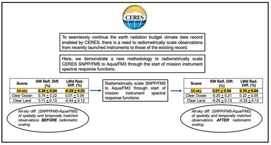
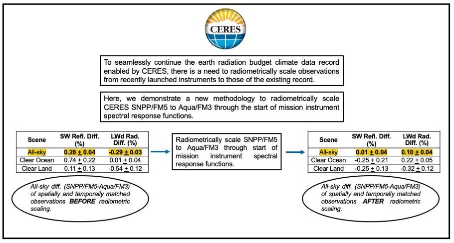
The ERB CDR from CERES is a combination of observations from Terra and Aqua after July 2002 [1]. To seamlessly continue this data record using observations from newly launched instruments onboard SNPP or NOAA-20, there is a need to radiometrically scale the measurements from these instruments to the observations forming the existing CDR. To radiometrically scale the Aqua instruments to Terra, the CERES team used a two-step process: (1) radiometrically scale Aqua/FM3 to Aqua/FM4 using direct comparison of simultaneous Earth observations from the two instruments, and (2) radiometrically scale Aqua/FM4 (and Aqua/FM3) using data from a special campaign conducted in July 2002 (the first month of Aqua’s mission) when both the Terra/FM1 and Aqua/FM4 instruments were placed in a programmable azimuth plane scan (PAPS) mode [4]. The PAPS mode of operation aligned both instruments’ scan plane to obtain observations of Earth in the vicinity of the orbital nodes. By obtaining the observational differences in the unfiltered radiances of all-scenes under all-sky conditions between Terra/FM1 and Aqua/FM4, radiometric scaling is achieved by applying a one-time systematic adjustment to each channel of both Aqua instruments to make their observations consistent with Terra/FM1.

In this work, the methodology to radiometrically scale SNPP/FM5 to Aqua/FM3 is described. The intersatellite comparison methodology to compute the differences between SNPP/FM5 and Aqua/FM3 observations while simultaneously viewing the same scene is provided. In Section 3, the process to place the SNPP/FM5 instrument on the same radiometric scale as the Aqua/FM3 instrument is described, and in Section 4, the results after the radiometric adjustment are shown. In Section 5, the long-term consistency trends between SNPP/FM5 and the instruments aboard Terra and Aqua are demonstrated.

2. Aqua-SNPP Intersatellite Comparisons

In the case of Aqua and SNPP, the altitudes (Aqua at 705 km and SNPP at 824 km) and orbital inclinations (Aqua-98.2° and SNPP-98.7°) of the spacecraft are such that their orbits crossover about every 64 h. This provides a large set of overlapping observations of the Earth from both instruments (SNPP/FM5 and Aqua/FM3) over diverse geographical regions that can be compared. Criteria to subset footprints that are considered matched are established—viewing and solar zenith angle differences of < 2°, relative azimuth of < 5°, and latitude and longitude difference of < 0.05°. The latitude and longitude constraints ensure the selection of the same geolocation, the viewing zenith and relative azimuth constraints ensure the two instruments view the scene with similar viewing geometries, while the solar zenith constraints provide a time constraint between the observations from the two instruments. Further, the comparisons are discretized by surface types (ocean and land) and cloud coverage (clear and all-sky), providing further insight into the spectral nature of the differences between the measurements of the two instruments.

For the SW, the differences are computed on a footprint basis on the reflectance (R), derived from the SW unfiltered radiances as shown in Equation (1) below:

$$R=\frac{SWrad*\pi }{F*\cos \left(SZA\right)}$$

(1)

where SWrad represents the SW unfiltered radiance, F = 1361 W/m² is a fixed value used for the solar irradiance at the Earth’s TOA, and SZA is the solar zenith angle at the Earth footprint under consideration. For the longwave (LW), the differences are computed on the unfiltered radiances on a footprint basis. For the daytime LW, these are obtained using the TOTc and SWc measurements [5], while for the nighttime, they are obtained directly from the TOTc. The global yearly differences are computed from daily averages from matched footprints (based on the criteria above). The computations are performed using the CERES Single Scanner Footprint (SSF) data products, with Aqua/FM3 using the Edition-4 while SNPP/FM5 uses the Edition-1 versions of these data products.

In the manner described above, the magnitude and spectral nature of scaling necessary are first determined. The yearly average SW reflectance and LW radiances for daytime and nighttime are computed for observations from each instrument, separated by scene types: clear-sky ocean, clear-sky land, and all-sky, and then differenced for each year starting from 2012 (the first full year of SNPP data). During the analysis of the data, it was determined that the observations from 2014 provided greater number of matched SNPP/FM5 and Aqua/FM3 samples than either 2012 or 2013. Hence the data from 2014 are used for analysis and application of radiometric scaling. The differences between the SNPP/FM5 and Aqua/FM3 SW reflectance and LW radiances for 2014 are summarized in

Table 1. Differences in the global average shortwave (SW) reflectance, daytime longwave (LWd) and nighttime LW (LWn) radiance between Suomi National Polar-orbiting Partnership (SNPP)/Flight Model (FM) 5 Single Scanner Footprint (SSF) Edition-1 and Aqua/FM3 SSF Edition-4 data products in 2014 for the three scenes considered. Differences shown are FM5-FM3, as a percentage along with the 95% confidence intervals.

Scene	FM3 SW Mean Refl.	SW Refl. Diff. (%)	FM3 LWd Rad. Mean (Wm−2sr−1)	LWd Rad. Diff. (%)	FM3 LWn Rad. Mean (Wm−2sr−1)	LWn Rad. Diff. (%)
All-Sky	0.2939	1.39 ± 0.06	77.44	−0.54 ± 0.04	73.67	−0.09 ± 0.01
Clear Ocean	0.0605	2.75 ± 0.22	91.30	−0.08 ± 0.04	93.16	−0.22 ± 0.03
Clear Land	0.2180	0.94 ± 0.14	101.56	−0.66 ± 0.14	88.23	−0.14 ± 0.02

.

The data in Table 1 indicate that the SW reflectance from SNPP/FM5 is consistently higher than those for Aqua/FM3, with all-sky differences of 1.39 ± 0.06%, the daytime LW radiances are consistently lower than those for Aqua/FM3, with all-sky differences of –0.54 ± 0.04%, and the nighttime LW radiances differences are small, with all-sky differences of –0.09 ± 0.01%. The nighttime LW radiance differences are small enough such that no radiometric adjustment is necessary to the SNPP/FM5 TOTc.

Prelaunch calibration data used for the generation of SNPP/FM5 beginning of mission (BOM) SRFs were reanalyzed due to minor errors identified in the algorithm for the computation of the average sensor counts while staring at the SW calibration source. This impacted the BOM SRFs for the SWc and the SW portion of the TOTc, while the LW portion of the TOTc was unaffected.

Table 2. Differences in the global average SW reflectance and daytime LW (LWd) radiance between SNPP/FM5 SSF Edition-1 data product with new beginning of mission (BOM) SRFs and Aqua/FM3 SSF Edition-4 data product in 2014 for the three scenes considered. Differences shown are FM5-FM3, as a percentage along with the 95% confidence intervals.

Scene	SW Refl. Diff. (%)	LWd Rad. Diff. (%)
All-sky	0.28 ± 0.04	−0.29 ± 0.03
Clear Ocean	0.74 ± 0.22	0.01 ± 0.04
Clear Land	0.11 ± 0.13	−0.54 ± 0.12

shows the recomputed SW reflectance and daytime LW radiance differences between Aqua/FM3 and SNPP/FM5 when using the new BOM SRF. The nighttime LW radiances were unaffected and were identical to those shown in Table 1. The SNPP/FM5 SW and daytime LW unfiltered radiances were computed using filtered radiances obtained from the SNPP/FM5 SSF Edition-1 data product and the new BOM SRF.

As seen in Table 2, the SW reflectance and daytime LW radiance differences using the new SNPP BOM SRFs are much smaller than those in Table 1. However, the SW difference observed for the clear-sky ocean scenes is significantly larger than those for all-sky or for clear-sky land scenes. Given that clear-sky ocean scenes have a larger percentage of energy in the shorter (blue) wavelengths, the larger SW difference for clear-sky ocean scenes compared to other scenes indicates discrepancies in the shorter wavelength regions of the SRFs between SNPP/FM5 and Aqua/FM3. The goal is to apply a radiometric scaling to SNPP/FM5 that would produce near-zero difference for all-sky comparisons and small differences for other clear-sky scenes. The daytime LW unfiltered radiances are computed using both the TOTc and the SWc measurements. Therefore, we first scale the SWc and then compute the resulting daytime LW difference and adjust the TOTc SRF as needed. The nighttime LW differences for all-sky all-scenes is small (based on the Edition-1 results in Table 1). Hence, no radiometric adjustments are necessary to the TOTc in the longer wavelengths.

To scale the SNPP/FM5 SWc, a simple broadband radiometric scaling will not be adequate since the differences depend on the scene type under consideration. The scaling will thus need to be spectral in nature such that adjustments need to be made to the BOM SRF of SNPP/FM5 SWc (within uncertainty) to achieve the desired result. The methodology to achieve the necessary scaling through adjustments to the BOM SRFs is described in the next section.

3. Radiometric Scaling through Spectral Response Function Adjustments

As discussed above, the radiometric scaling needs to be applied through adjustments to the prelaunch BOM SWc SRF for SNPP/FM5 such that the resulting computed all-sky SW reflectance matches the Aqua/FM3 value shown in Table 2. The BOM SWc SRF generation process for the spectral range of 0.3 to 2 µm using a broadband lamp and 13 narrow band filters is described in Appendix A. The radiometric scaling is performed through adjustments to the CERES measurements in the 13 filter bands within their uncertainties. A Lagrange multiplier objective constrained optimization algorithm is used to obtain the solution for the amount of adjustment for each filter band [6]. This algorithm is described below.

3.1. Radiometric Scaling Algorithm

If R_FM5 and R_FM3 represent the SW reflectance for SNPP/FM5 and Aqua/FM3, respectively, the relationship between the two is expressed as:

$$R_{FM5}-E_R=R_{FM3}$$

(2)

where E_R is the adjustment to the SNPP/FM5 global all-sky all-scenes reflectance that is necessary to match that of Aqua/FM3. The adjustment is performed within uncertainties in the SNPP/FM5 SRF, p_i, where i corresponds to one of the 13 wavelength bands used during the prelaunch BOM SRF determination. p_i is modified by some amount x_i such that the reflectance ${\widehat{R}}_{FM5}$ calculated with the new SRF is equal to R_FM3. This means:

$${\widehat{R}}_{FM5}=R_{FM5}-\sum _i\frac{\partial R_{FM5}}{\partial p_i}{x}_i=R_{FM3}$$

(3)

This requires finding x_i such that

$$\sum _i\frac{\partial R_{FM5}}{\partial p_i}{x}_i=E_R$$

(4)

Let a_i = $\frac{\partial R_{FM5}}{\partial p_i}$ denote the partial derivatives of the mean reflectance with respect to each parameter p_i, and represent x_i and a_i as vectors x and a, then Equation (4) can be written as

$$a^{t}x=E_R$$

(5)

There is one equation with 13 unknowns, representing the wavelength bands to which adjustments can be made to provide the desired reflectance value. To determine the amount of adjustment necessary in each wavelength band, x_i, a maximum likelihood estimator is used while making the following assumptions: (1) x_i has zero mean for all i; and (2) x_i’s are normally distributed. The probability distribution function for x_i can be written as:

$$P\left\{x\right\}={\left(2\pi \right)}^{-n/2} {\left[\det \left(C\right)\right]}^{-1/2} \exp \left(-x^t{C}^{-1}x/2\right)$$

(6)

where C is the covariance matrix of the errors. The most likely set of errors is obtained by maximizing the probability P(x), which occurs when the exponent of Equation (6) is maximized. The method of Lagrangian multipliers is used to determine the solution, whereby

$$\mathsf{\Omega }=\frac{1}{2}{x}^t{C}^{-1}x+\lambda a^{t}x$$

(7)

is minimized; where $\lambda$ is the Lagrangian multiplier. The maximum likelihood solution is

$$x= -\lambda Ca$$

(8)

This, when used with Equation (5), gives

$$\lambda ={(a^{t}Ca)}^{-1}{E}_R$$

(9)

It is assumed that all error terms are uncorrelated and thus the covariance matrix C is diagonal. The Lagrangian multiplier then becomes

$$\lambda =\frac{E_R}{{\sum }_i{a}_i{}^2{\delta }_i{}^2}$$

(10)

where ${\delta }_i$ is the uncertainty in the i^th parameter. The maximum likelihood solution is determined as

$$x_i=-\lambda a_i{\delta }_i^2$$

(11)

The terms a_i and ${\delta }_i$ are the uncertainty of the spectral responsivity and the reflectance uncertainty, respectively. A description of how these terms are obtained using prelaunch calibration data are described in Appendix A and Appendix B.

3.2. Optimal Solution for SWc SRF

The algorithm described above and data from

Table A1. Spectral responsivity uncertainty (a_i) and the Reflectance uncertainty (${\delta }_i$ ) for global all-sky, as a function of filter center wavelength, obtained using SNPP/FM5 prelaunch calibration data and inter-comparison data sets, for the year 2014 (adapted from [6]).

Filter Center Wavelength (µm)	$\mathbf{Spectral} \mathbf{Responsivity} \mathbf{Uncertainty} \left({\mathbf{a}}_{\mathbf{i}}\right) (2-\mathit{\sigma }) (\%)$	ΔReflectance (%)	$\mathbf{Reflectance} \mathbf{Uncertainty} ({\mathit{\delta }}_{\mathit{i}}$$) (2-\mathit{\sigma }) (\%)$
0.42	1.9	−0.277	−0.527
0.46	1.3	−0.071	−0.092
0.52	0.9	−0.057	−0.052
0.62	0.1	−0.105	−0.010
0.72	0.1	−0.132	−0.013
0.81	0.3	−0.132	−0.040
0.90	0.1	−0.085	−0.008
1.00	0.2	−0.044	−0.009
1.14	0.3	0.000	0.000
1.26	0.5	−0.020	−0.010
1.35	0.7	−0.057	−0.040
1.64	1.0	−0.020	−0.020
1.95	1.0	−0.014	−0.014

(Appendix B) are used to determine the adjustments necessary in each filter band to obtain the desired global all-sky SW reflectance for SNPP/FM5. The results are tabulated in

Table 3. Maximum likelihood solution for the adjustments to the spectral responsivity for each of the 13 filter bands to radiometrically scale the SWc of SNPP/FM5 to Aqua/FM3 for global all-sky using the intercomparison dataset for 2014 (adapted from [6]).

Filter Center Wavelength (µm)	Maximum Likelihood Solution xi (%)	Spectral Responsivity Adjustment (%)
0.42	0.3725	1.339
0.46	0.0114	0.161
0.52	0.0036	0.062
0.62	0.0002	0.001
0.72	0.0002	0.002
0.81	0.0021	0.016
0.90	0.0001	0.001
1.00	0.0001	0.002
1.14	0.0000	0.000
1.26	0.0001	0.007
1.35	0.0022	0.038
1.64	0.0006	0.027
1.95	0.0003	0.018

(adapted from [6]). The maximum likelihood solution, x_i, is the amount of change necessary in each filter band. Shown as well are the amount of adjustments necessary to the spectral responsivity in each of the filter bands to obtain the desired reflectance for SNPP/FM5. The target reflectance for SNPP/FM5 is the same as that of Aqua/FM3 for global all scenes under all-sky conditions, 0.2939 (from Table 2), the Lagrangian multiplier value, λ = –455.52, and the value of a_i set to the current value of the SNPP/FM5 reflectance for all filter bands, before any radiometric adjustments, 0.2947 (computed from Table 2). It should be noted that the amount of adjustment in all of the filter bands is smaller than their corresponding 2-sigma uncertainty values (shown in column 2 in Table A1 (Appendix B)).

4. Results

4.1. Differences for 2014

Using the optimal solution obtained in Table 3 above, a new BOM SNPP/FM5 SWc SRF is generated by applying the required adjustments to the spectral responsivities. To verify that the required radiometric scaling is obtained, the SW reflectance and daytime LW radiance differences are recomputed using the SNPP/FM5-Aqua/FM3 intercomparison data while using the same approach described in Section 2. The results are shown in

Table 4. Differences in the global average of SW reflectance and daytime LW (LWd) radiance between SNPP/FM5 after radiometric scaling and Aqua/FM3 Edition-4, for 2014 for the three scenes considered. Differences shown are FM5-FM3, as a percentage along with the 95% confidence intervals.

Scene	SW Refl. Diff. (%)	LWd Rad. Diff. (%)
All-sky	0.01 ± 0.04	0.10 ± 0.04
Clear Ocean	−0.25 ± 0.21	0.22 ± 0.05
Clear Land	−0.25 ± 0.13	−0.32 ± 0.12

, for the three scenes, for 2014.

It is seen that global all-sky SW reflectance for SNPP/FM5 are in good agreement with Aqua/FM3 for the data considered. While the differences for clear-sky ocean differences have reduced from a mean value of 0.74% to –0.25%, the clear-sky land scenes have shown a marginal increase in differences from 0.11% to –0.25%. The daytime LW radiances for all-sky, 0.10 ± 0.04%, show good agreement based on the scaling in the SWc thus precluding the need for any further adjustments to the TOTc. The differences for the ocean and land scenes are small relative to the overall accuracy budget.

4.2. Long-Term Differences

The long-term differences between SNPP/FM5 and Aqua/FM3 are observed over the years 2012–2019 using yearly average of matched footprints when the two spacecraft orbits crossover. The radiometric scaling to the SNPP/FM5 SWc impacts the monthly daytime LW fluxes but does not affect their long-term trends. In looking at the long-term trends of daytime LW global all-sky flux differences between SNPP/FM5 and Aqua/FM3, a trend of 0.53 ± 0.16 Wm⁻²/decade was observed [6]. The trends were attributed to the SW portion of the TOTc since it was shown that the flux difference trends for the SW were not statistically significant. This necessitated the application of a time-varying change to the TOTc SRF, similar to those being applied to the TOTc for the instruments on Terra and Aqua [7]. These time-varying SRF changes for the TOTc along with the radiometric scaling for the SWc have been incorporated in the soon to be released Edition-2 SNPP/FM5 SSF data products.

Due to delays in release of Collection-2 Visible Infrared Imaging Radiometer Suite (VIIRS) data, the release of the CERES Edition-2 SSF data products for SNPP/FM5 have taken longer than expected. To validate the new BOM and time-varying SRFs for SNPP/FM5, the unfiltered radiances (and fluxes) are computed using the filtered radiances and imager parameters in the Editon-1 SSF data products. An offline product is created similar to the SSF-1deg product (called preEdition-2 for the purposes of this paper). It is expected that the results from the offline runs will closely represent the results from the Edition-2 data products.

Using the subset data when the orbits of SNPP/FM5 and Aqua/FM3 crossover, the matched footprints are analyzed using the criteria and methodology described in Section 2. The differences between the SW reflectance and daytime LW unfiltered radiances for global all-sky are presented. The data products used for this analysis are Edition-4 SSF data products for Aqua/FM3 and preEdition-2 for SNPP/FM5. The results are shown in

Table 5. Differences in the global average of all-sky SW reflectance and daytime LW (LWd) radiance between SNPP/FM5 preEdition-2 and Aqua/FM3 Edition-4, for the years 2012–2019. Differences shown are FM5-FM3, expressed as a percentage along with the 95% confidence intervals.

Year	SW Refl. Diff. (%)	LWd Rad. Diff. (%)
2012	−0.29 ± 0.07	−0.14 ± 0.05
2013	−0.33 ± 0.07	−0.13 ± 0.04
2014	0.01 ± 0.04	0.10 ± 0.04
2015	0.02 ± 0.05	0.03 ± 0.04
2016	−0.05 ± 0.06	−0.06 ± 0.03
2017	−0.07 ± 0.06	−0.17 ± 0.04
2018	−0.08 ± 0.07	−0.10 ± 0.03
2019	−0.17 ± 0.05	−0.17 ± 0.04

for years 2012 through 2019.

It is seen that there is very good agreement between SNPP/FM5 and Aqua/FM3 for the year 2014, the dataset used for the radiometric scaling. For 2014 and beyond, the differences for both SW and daytime LW are within 0.2%, thus showing very good consistency in performance between the two instruments for all years since the radiometric scaling was applied.

5. Consistency of CERES Instrument Performance

The performance of SNPP/FM5 is compared with the CERES instruments on Terra and Aqua by looking at the long-term trends in global flux anomalies. Due to delay in availability of the official Edition-2 data products for SNPP, the results are shown using the Edition-1 products first, and then the results between the Edition-1 and preEdition-2 products are compared.

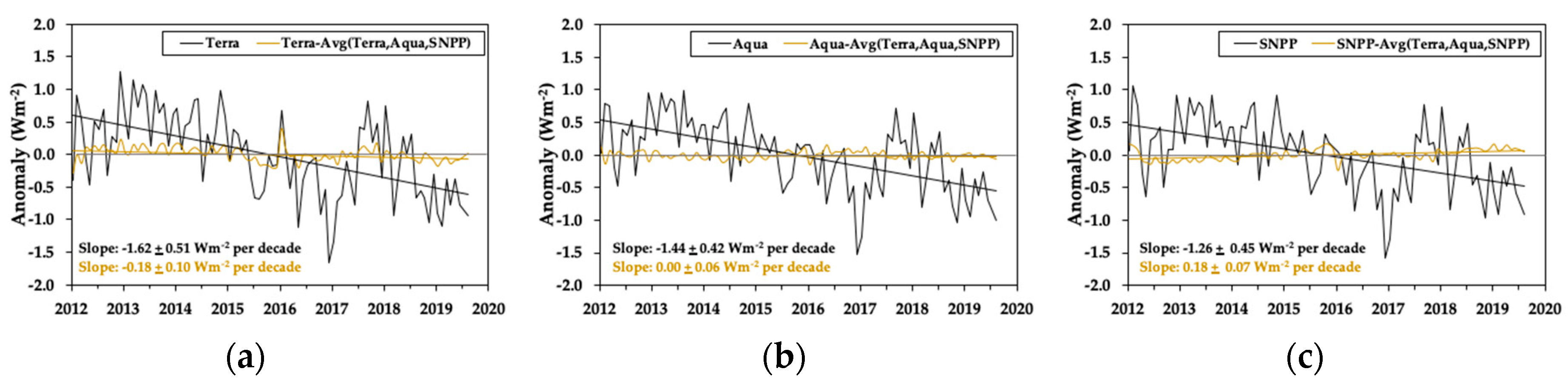
The anomalies of the SW global fluxes are computed and the long-term trend with time using the same climatological record: 02/2012 through 09/2019 for all instruments for all-sky (Figure 1) are compared. In August 2019, the SNPP/FM5 instrument was placed in the rotating azimuth plane scan (RAPS) mode and no science observations were available for a part of that month, and therefore, August 2019 is excluded during the computation of the anomaly for both SNPP/FM5 and Aqua/FM3. SNPP/FM5 has been operating in RAPS mode since October 2019; therefore, results are presented only through September 2019. The comparison is carried out using the SSF1-deg products with Edition-4 for Terra and Aqua, and Edition-1 data products for SNPP, to demonstrate the performance of SNPP/FM5 before applying the SRF corrections. Additionally, shown on the plots are the differences between the individual instrument anomalies and the anomaly of the average of all three instruments.

All three CERES instruments show a large decrease in reflected SW radiation for the period considered. This trend is associated with short-term interannual variability rather than a long-term trend [8]. It is noted that differences in the trends amongst the three CERES instruments is at least a factor of seven smaller than the trend itself and remains < 0.18 Wm⁻² per decade. Part of this small difference could be due to differences in diurnal sampling between Terra (10:30 a.m. equator crossing time) and Aqua or SNPP (1:30 p.m. equator crossing time).

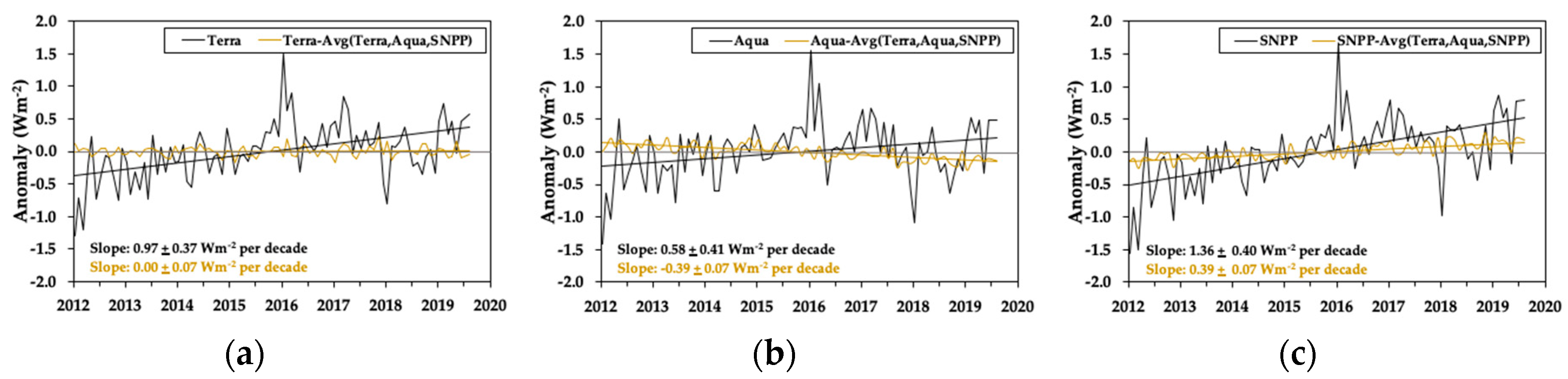
The LW anomaly trends for the three instruments are shown in Figure 2. Additionally, shown is a comparison of the individual trends with the trends using the average of the three instruments. These plots are generated using the SSF-1deg data products with Terra and Aqua using Edition-4 and the SNPP using Edition-1. The SSF-1 deg product combines the daytime and nighttime observations into a single LW flux.

All instruments show a significant positive trend with SNPP showing 1.36 ± 0.40 Wm⁻² per decade. The TOTc for SNPP/FM5 are uncorrected in that no SRF changes have been incorporated in the Edition-1 data products, resulting in larger slopes of the trends with time. The largest difference between the slope of the anomaly from any single instrument and the slope of the anomaly of the average of all three instruments is 0.39 Wm⁻² per decade with Aqua showing a negative slope and SNPP, a positive slope.

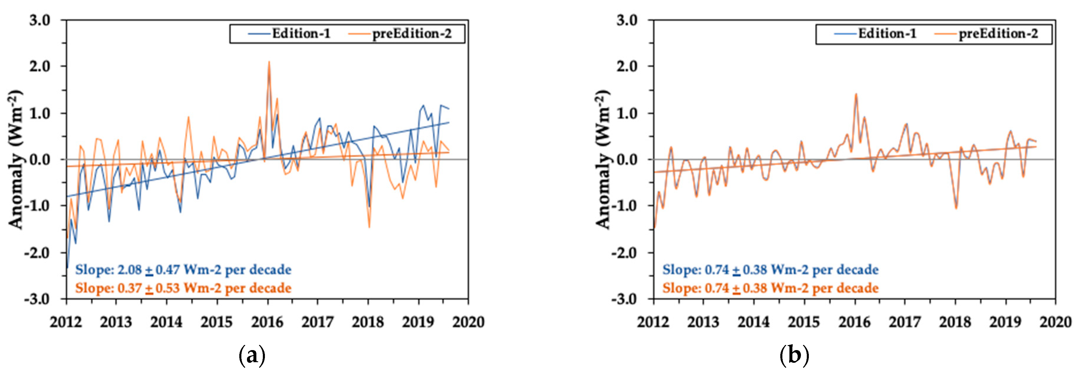
To provide a sense of the magnitude of the changes incorporated into the Edition-2 data products for SNPP/FM5, the preEdition-2 SSF data product is used. The LW anomalies are computed for the same time period and compared with Edition-1. The computation of the LW flux for Edition-2 incorporates the time varying SRFs applied to the TOTc. For this comparison, the monthly global TOA LW fluxes for both daytime and nighttime periods are considered, as shown in Figure 3. The SW anomalies are not shown because they are identical to those from Edition-1. The radiometric scaling to the SWc is a systematic adjustment and results in no change to the long-term anomalies or their trends with time.

The addition of the time varying SRF corrections in the TOTc for SNPP/FM5 significantly reduces the slope in the long-term trends of the anomalies of the daytime LW, from 2.08 ± 0.47 Wm⁻² per decade to 0.37 ± 0.53 Wm⁻² per decade. The nighttime anomaly, which has a slope of 0.74 ± 0.38 Wm⁻² per decade, is unaffected by the application of the time-varying SRF. This is to be expected since the spectral corrections particularly impact the SW portion of the TOTc SRF, which only manifests as changes to the daytime LW, while keeping the nighttime LW unchanged.

6. Conclusions

The CERES instruments continue to provide crucial measurements to enable a multi-decadal climate data record of the Earth’s radiation budget. The climate data record combines observations from the CERES instruments on Terra and Aqua from July 2002. To seamlessly continue the data record with more recently launched instruments on SNPP and NOAA-20, there is a need to radiometrically tie the observations from these instruments to the existing data record. In this work, a new approach to tie the observations from CERES FM5 flying on SNPP to the observations from FM3 on Aqua is presented. Spatially and temporally matched footprints from the two instruments when their orbits cross each other are used to determine the magnitude of radiometric scaling necessary. The methodology used a Lagrange multiplier based objective constrained optimization algorithm to find a unique solution to the required adjustments on the prelaunch calibration data (within measurement uncertainties) used to obtain the spectral response functions. The radiometric scaling is validated, and the remarkable consistency between the observations from the CERES instruments on Terra, Aqua, and SNPP is demonstrated. These newly released radiometrically scaled data products for SNPP have been validated and will soon be publicly available as Edition-2 versions of data products.

References

1. Loeb, N.G.; Doelling, D.R.; Wang, H.; Su, W.; Nguyen, C.; Corbett, J.G.; Liang, L.; Mitrescu, C.; Rose, F.G.; Kato, S. Clouds and the Earth’s Radiant Energy System (CERES) Energy Balanced and Filled (EBAF) Top-of-Atmosphere (TOA) Edition-4.0 Data Product. J. Clim. 2018, 31, 895–918. [Google Scholar] [CrossRef]
2. Priestley, K.J.; Barkstrom, B.R.; Bitting, H.C.; Lee, R.B., III; Pandey, D.K.; Thomas, S.; Thornhill, K.L. End-to-end spectral characterization of the Clouds and the Earth’s Radiant Energy System (CERES) thermistor bolometer radiometers. Proc. SPIE 1998, 3498. [Google Scholar] [CrossRef]
3. Priestley, K.J.; Smith, G.L.; Thomas, S.; Matthews, G. Validation protocol for climate quality CERES measurements. Proc. SPIE 2007, 6678, 66781I. [Google Scholar] [CrossRef]
4. Szewczyk, Z.P.; Priestley, K.J.; Walikainen, D.R.; Loeb, N.G.; Smith, G.L. Putting all CERES instruments (Terra/Aqua) on the same radiometric scale. Proc. SPIE 2011, 8177, 817704. [Google Scholar] [CrossRef]
5. Loeb, N.G.; Priestley, K.J.; Kratz, D.P.; Geier, E.B.; Green, R.N.; Wielicki, B.A.; Hinton, P.O.; Nolan, S.K. Determination of Unfiltered Radiances from the Clouds and the Earth’s Radiant Energy System Instrument. J. Appl. Meteorol. 2001, 40, 822–835. [Google Scholar] [CrossRef]
6. Shankar, M.; Priestley, K.J.; Smith, N.; Thomas, S.; Walikainen, D. Enabling continuity of the Earth radiation budget climate data record using the Clouds and Earth’s Radiant Energy System (CERES) Flight Model 5 on S-NPP. Proc. SPIE 2019, 11127, 111270Y. [Google Scholar] [CrossRef]
7. Loeb, N.G.; Manalo-Smith, N.; Su, W.; Shankar, M.; Thomas, S. CERES Top-of-Atmosphere Earth Radiation Budget Climate Data Record: Accounting for in-Orbit Changes in Instrument Calibration. Remote Sens. 2016, 8, 182. [Google Scholar] [CrossRef] [Green Version]
8. Loeb, N.G.; Thorsen, T.J.; Norris, J.R.; Wang, H.; Su, W. Changes in earth’s energy budget during and after the “pause” in global warming: An observational perspective. Climate 2018, 6, 62. [Google Scholar] [CrossRef] [Green Version]
Figure 1. SW global all-sky flux anomalies for the period February 2012–September 2019 using the SSF-1deg products for: (a) Terra using the Edition-4 data products; (b) Aqua using the Edition-4 data products; and (c) S-NPP using the Edition-1 data products. Additionally, shown is the difference between the individual instrument anomalies and the anomaly of the average of the three instruments. Uncertainties in slope correspond to 95% confidence intervals.
Remotesensing 12 02787 g001
Figure 2. LW global all-sky flux anomalies for the period February 2012–September 2019 using the SSF-1deg products for: (a) Terra using the Edition-4 data product; (b) Aqua using the Edition-4 data product; and (c) S-NPP using the Edition-1 data product. Additionally, shown is the difference between the individual instrument anomalies and the anomaly of the average of the three instruments. Uncertainties in slope correspond to 95% confidence intervals.
Remotesensing 12 02787 g002
Figure 3. LW global all-sky flux anomalies for the period February 2012–September 2019 for SNPP using Edition-1 and preEdition-2 SSF products for: (a) daytime; (b) nighttime. Additionally, shown are the slopes of the trend with time and their corresponding 95% confidence intervals.
Remotesensing 12 02787 g003