Implementation of a Nowcasting Hydrometeorological System for Studying Flash Flood Events: The Case of Mandra, Greece

Abstract

Severe hydrometeorological hazards such as floods, droughts, and thunderstorms are expected to increase in the future due to climate change. Due to the significant impacts of these phenomena, it is essential to develop new and advanced early warning systems for advance preparation of the population and local authorities (civil protection, government agencies, etc.). Therefore, reliable forecasts of extreme events, with high spatial and temporal resolution and a very short time horizon are needed, due to the very fast development and localized nature of these events. In very short time-periods (up to 6 h), small-scale phenomena can be described accurately by adopting a “nowcasting” approach, providing reliable short-term forecasts and warnings. To this end, a novel nowcasting system was developed and presented in this study, combining a data assimilation system (LAPS), a large amount of observed data, including XPOL radar precipitation measurements, the Chemical Hydrological Atmospheric Ocean wave System (CHAOS), and the WRF-Hydro model. The system was evaluated on the catastrophic flash flood event that occurred in the sub-urban area of Mandra in Western Attica, Greece, on 15 November 2017. The event was one of the most catastrophic flash floods with human fatalities (24 people died) and extensive infrastructure damage. The update of the simulations with assimilated radar data improved the initial precipitation description and led to an improved simulation of the evolution of the phenomenon. Statistical evaluation and comparison with flood data from the FloodHub showed that the nowcasting system could have provided reliable early warning of the flood event 1, 2, and even to 3 h in advance, giving vital time to the local authorities to mobilize and even prevent fatalities and injuries to the local population.

1. Introduction

One of the climate change impacts is the increase of the likelihood and intensity of extreme weather events, such as floods, droughts, and thunderstorms [1,2] making human beings more vulnerable to extreme weather events [3]. The most common and destructive natural disaster is flooding, especially in a warm climate region like the Mediterranean Sea [4], causing loss of human life and substantial damage to property and infrastructure. In fact, more people were affected by floods than any other type of natural disaster in the 21st century [5] and the situation is expected to become worst in warm climates, as model simulations show that an increase in precipitation intensity is to be expected [6]. Moreover, intertemporal human-induced land cover changes seem to favor extreme weather phenomena, either droughts or floods, so there is the necessity to also take these into consideration in the future [7]. Early warning systems are being developed for advance preparation of the population and local authorities (civil protection, government agencies, etc.) to mitigate the effects of extreme weather hazards. A prime example is the Meteoalarm system, designed to give accurate information for advance preparation for extreme weather impacts over Europe [8]. The more recent Copernicus Emergency Management Service (EMS, regulation 377/2014) provides information for emergency response related to various types of hazards, from meteorological, geophysical, etc., to human-made disasters. EMS also helps with the prevention, preparedness, response, and recovery activities.

Reliable forecasts of extreme events at all scales, with high spatial and temporal resolution and a very short time horizon (up to 6 h) are important to reduce the risks and mitigate the effects of natural disasters [1]. In such a short time-period, small-scale phenomena can be described accurately by adopting a “nowcasting” approach. The term nowcasting usually describes weather forecasts in a very short time horizon, with high spatiotemporal resolutions [9,10,11,12]. These types of short-time forecasts are valuable to Civil Protection services and local authorities for use in early warning systems [13,14]. They give the opportunity to Civil Protection to implement immediate plans and policies, in order to mitigate property losses and protect human lives [15].

Nowcasting methods usually focus on the estimation of precipitation [16]. Precipitation can be measured either directly with the use of ground-based instruments (for example rain gauges) or indirectly with the use of remotesensing techniques like radar systems, Earth-observing satellites, TRMM (Tropical Rainfall Measuring Mission), and GPM (Global Precipitation Measurement). One of the first attempts for nowcasting was the forward-time extrapolation of ground-based radar rainfall data [17], which gradually expanded to include high-resolution data provided by numerical models, using assimilation systems [18,19]. One of the first regional nowcasting systems was the Rapid Update Cycle (RUC) in 1994, which combined an 80 km horizontal grid spacing with a 3 h radar data acquisition [18]. The first test of such a rainfall short-time forecasting system took place in the 2000 Summer Olympics in Sydney, using only radar-data-based quantitative precipitation nowcasting algorithms [20]. Six years later, it was found that accurate forecasts could be achieved by applying data assimilation of real-time radar reflectivity and Doppler velocity fields [21].

Data assimilation includes a statistical combination of observations and short-term forecasts. The state of the atmosphere is estimated through a combination of computer simulations and real observations. The data assimilation cycle is then repeated and new observations are embodied to make a new analysis of the atmospheric state [22]. Therefore, the purpose of this process is to combine past knowledge of the system, in the form of numerical model fields, and new information about the system, in the form of observations [23]. In this way, the value of hypothetical observations could be estimated with data assimilation [24,25].

Some examples of nowcasting methods include—the object-based algorithm, Thunderstorm Identification Tracking Analysis and Nowcasting (TITAN), which identifies and tracks storm cells [26] and ingests radar data remapped into Cartesian coordinates. An area-based method is the Collaborative Adaptive Sensing of the Atmosphere radar network (CASA) [27] that uses X-band weather radar data, where the precipitation motion is estimated by the Dynamic and Adaptive Radar Tracking of Storms (DARTS) method. The linear least squares estimation is used in the Fourier domain to compute the precipitation pattern. Secondly, a kernel-based advection method is implemented to estimate the motion. The Integrated Nowcasting through Comprehensive Analysis (INCA) system is a statistical model that uses a multiple observation system and combines remotesensing data with surface station data and topographic data [28]. An example of application of actual data with a modelling system is the Short-Term Ensemble Prediction System (STEPS), which is a probabilistic nowcasting system [29,30]. It blends weather radar data and forecasts from a mesoscale Numerical Weather Prediction (NWP) model to produce ensembles of precipitation forecasts. Similarly, the Application of Research to Operations at Mesoscale (AROME) [31] model uses Euler equations (non-hydrostatic versions) and a 3DVar assimilation scheme that assimilates radar and satellite data. All systems presented above either lack a numerical weather prediction model, or a hydrological component in their framework for precision flood warnings. In this work, a novel nowcasting methodology is proposed, based on a well-known assimilation model, namely the Local Analysis and Prediction System (LAPS) [32,33], coupled with the Chemical Hydrological Atmospheric Ocean wave System (CHAOS) [34,35,36,37,38] currently including, among others, the Advanced Weather Research Forecasting (WRF-ARW) version 4.0 model [39,40] as an atmospheric component and the WRF-Hydro version 3.0 model [41] as a hydrological component. The LAPS model uses WRF-ARW’s forecasts as background fields assimilating various observations like radar data, so as to force WRF-Hydro, finally creating a “state-of-the-art”, fast, and reliable early warning system for hydrometeorological hazards.

The developed system was used to assess very short-term precipitation and discharge predictions in the case study of the catastrophic flash flood event that occurred in the sub-urban area of Mandra in Western Attica, Greece, on 15 November 2017. The selection of the event was based on the severity of the flash flood, which caused 24 people to lose their lives and inflicted extensive million-euro damages on property and infrastructure. This event was recorded as the deadliest flood in the country, in a period of 40 years [42], highlighting the necessity of hydrometeorological hazard early warnings at the wider region [43]. This event was already described in detail in Varlas et al. [36], where the importance of utilizing radar data in order to provide a reliable short-term forecast of extreme hydrometeorological events was highlighted. Therefore, this work was the continuation of Varlas et al. [36], as the severity of the event made it ideal for testing and evaluating the proposed nowcasting system. This manuscript is organized as follows. In Section (2), the study area is presented, along with a short description of the event. Section (3) describes the numerical systems and data used. In Section (4), the methodology and experimental design are shown, while the results and evaluation are presented in Section (5). Finally, in Section (6) we discuss the conclusions and implications of the study.

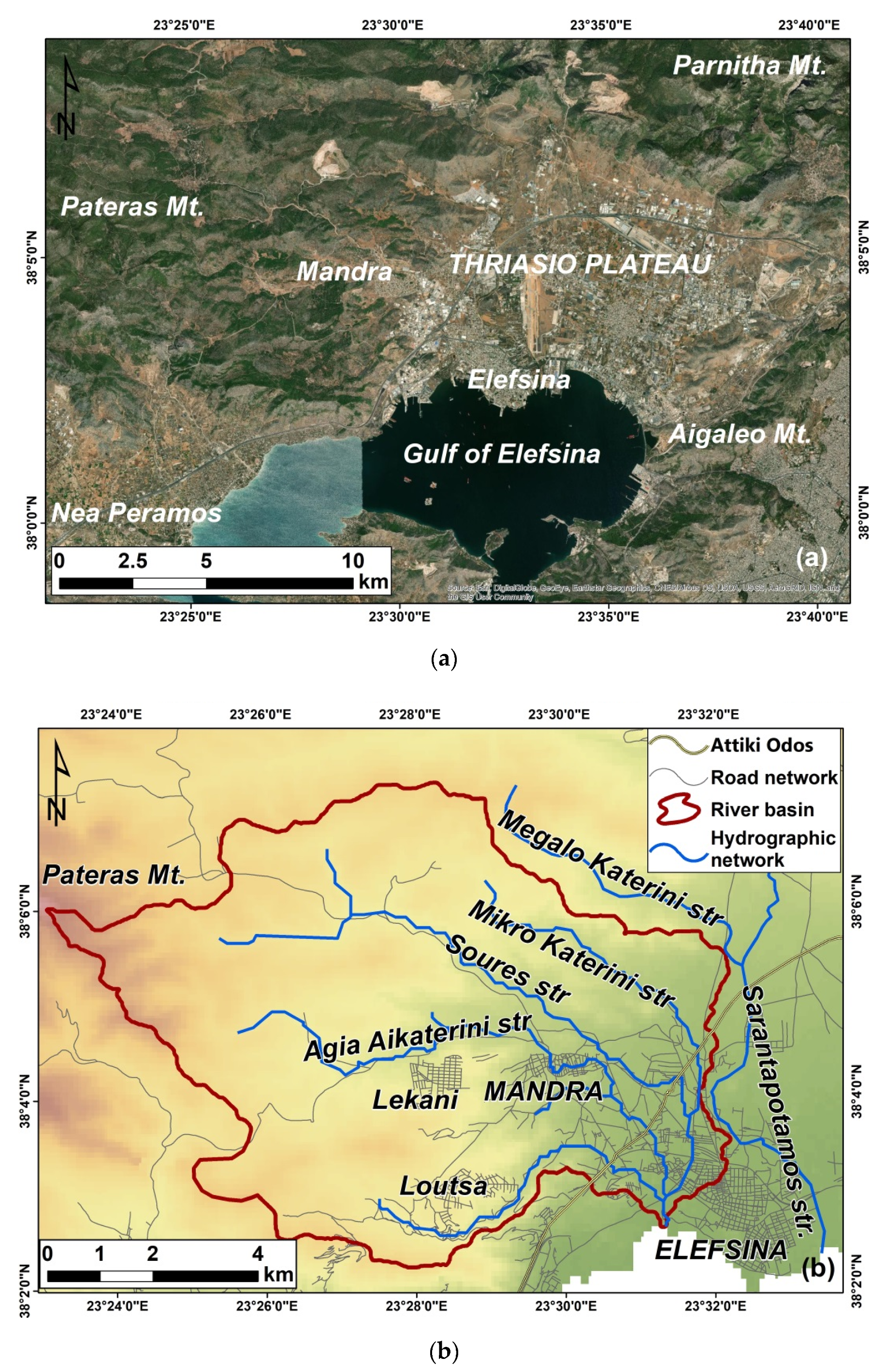
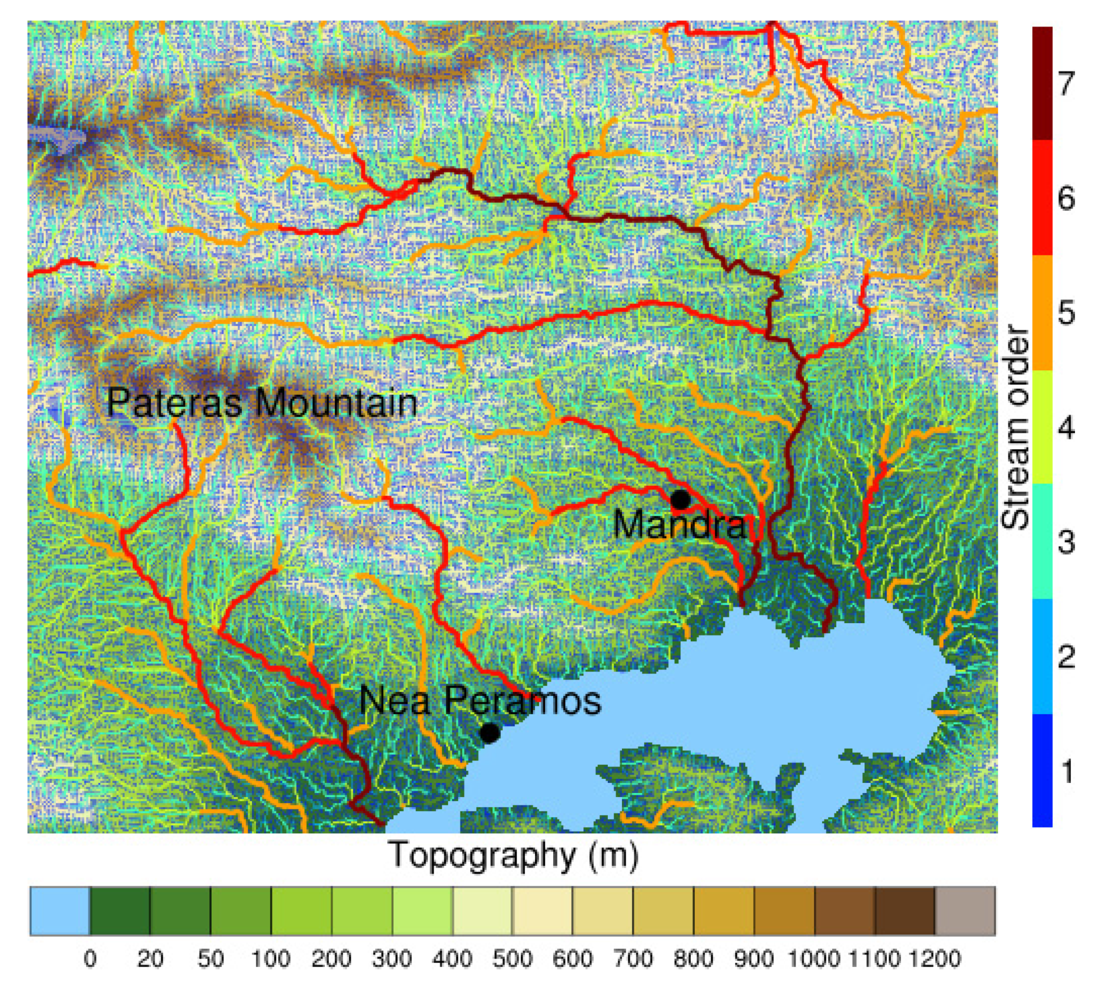
2. Study Area and Description of the Flood Event

In the morning of 15 November 2017, a severe thunderstorm caused a flash flood in the town of Mandra in Western Attica. Mandra is located is 40 km west of Athens and is an industrial town, with a population of approximately 13,000 people. As presented in Figure 1a, the area is bound by the Pateras Mountain (1016 m) in the west, the Parnitha Mountain (1413 m) in the northeast, and the Aigaleo Mountain (468 m) in the east [36]. The town is located at the apex of an alluvial fan, formed by two streams at the western part of the Thriassio plain, which meet at the southeastern edge of the town to form a stream that ends at the Gulf of Elefsina (Figure 1a). In Figure 1b the Agia Aikaterini, Soures and Sarantapotamos streams near Mandra are presented, in the context of the greater area. It is noteworthy that the town is characterized by significant morphological changes of the streams, due to uncontrolled building and road works interrupting the streams Figure 1b, as the residential and industrial development did not have an appropriate plan regarding flood protection and drainage rainwater collection [44]. Human-induced morphological changes in Mandra, in combination with the high rainfall rate, played a key role in the triggering and evolution of the flood [36,42,45].

The dominant atmospheric mechanism that led to the heavy rainfall that caused the flood, was the convergence of humid south-southeasterly airflow over the southeastern slopes of the Pateras Mountain [36]. Near-surface convergence was collocated with the favorable middle-upper air conditions supporting persistent torrential rainfall, for approximately 5 h east of the Pateras Mountain, which increased surface water runoff and stream discharge. The storm was also supported by a stagnant spinning barometric low, preserving both the humid south-southeasterly airflow near the surface, as well as the favorable middle-upper air conditions. A detailed analysis of the event is presented in great detail in Varlas et al. [36] and are not repeated in this study.

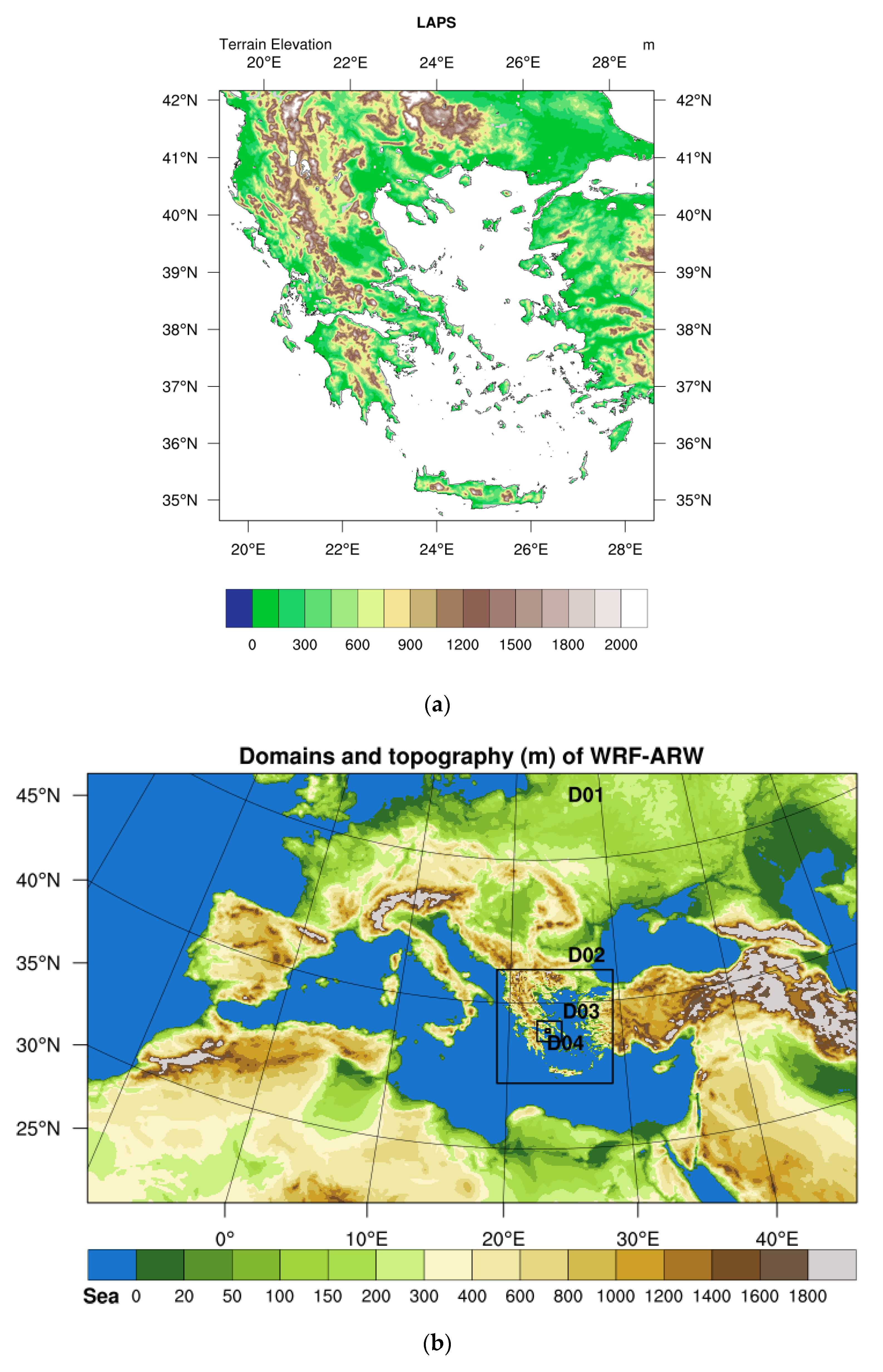
3. Materials Used and System Development

The development of the early warning system presented here is based on the combination of highly accurate and reliable measurements, a well-known and established data assimilation system coupled with a weather model and a hydrological model. All components used are presented below.

3.1. Local Analysis and Prediction System (LAPS) and Precipitation Advection

NOAA’s Local Analysis and Prediction System (LAPS) is an advanced mesoscale meteorological data assimilation tool, designed to exploit all available data sources (local and global) and produce analyzed and guessed grids [32]. LAPS can ingest a wide range of available observational data. (a) Surface observation data including mesonet, METAR, SYNOP, maritime (Buoy/Ship), and others; (b) profiler data like RASS, SODAR, and Wind Profilers; (c) satellite data like GOES or METEOSAT, cloud drift winds; (d) satellite sounder data; (e) radar data like 3D Reflectivity, Doppler radars, radar VAD Algorithm winds database, and low-level reflectivity; and (f) ACARS and PIREPS from aircraft [46,47]. User specific datasets can also be added in the assimilation framework with some additional coding and modifications. When the actual observational data are available, LAPS can then use the background fields from a number of sources (GFS, ECMWF, etc.), as the first-guess meteorological fields. The assimilation methodology was based on the traditional objective analysis scheme, using the cost-function approach, in order to minimize differences between the analysis and the observational fields. Barnes [48] also introduced an empirical methodology of successive corrections, which can be used when the background field or the first guess was not available.

In the framework of LAPS, a simple advection scheme was added to forecast the movement of rain, for a horizon of 1–3 h. The development was based on a simple first-order advection scheme in 2 dimensions (x, y):

$$\frac{1}{\Delta t}(R_{i,j}^{t+1}-R_{i,j}^t)+\frac{u}{\Delta x}(R_{i,j}^t-R_{i-1,j}^t)+\frac{v}{\Delta y}(R_{i,j}^t-R_{i,j-1}^t)=0$$

(1)

where u and v the wind components, R is the precipitation, Δx is the grid increment in the x direction, Δy is the grid increment in the y direction, Δt is the timestep, and (i, j) are the grid point in the LAPS domain. A stability analysis shows the scheme to be conditionally stable, when

$$CU=u\frac{\Delta t}{\Delta x}\ge 0$$

(2)

$$CV=v\frac{\Delta t}{\Delta y}\ge 0$$

(3)

where CU and CV the Courant numbers in the x and y directions, respectively, with restriction of CU + CV ≤ 1. At each timestep, the Courant number was calculated in order to check if the timestep selected assured the stability of the formulation, and by solving Equations (1)–(3), the value of the parameter R at time t + 1 was estimated. The benefit of the applied methodology was that the updated LAPS could overcome the ‘spin up’ period, which routinely appeared in the conventional numerical weather prediction mesoscale models. The drawback was that the scheme was unsuitable for use beyond the 3-h forecasting horizon, since there were no additional physical parameterizations included. After the forecast horizon, the dynamical processes could not be ignored anymore and the results could not be safely used (especially in small spatial scales).

For the needs of this work, LAPS was set up with a fine resolution of 2 km, covering Greece (Figure 2). On the vertical plane, 42 constants pressure levels were defined, stretching from the surface to the top of the atmosphere. Global geography datasets were used for topography, land fraction, land use (U.S Geological Survey dataset with a resolution of 30 s), soil type, greenness fraction [49], and albedo definition [50].

LAPS is primarily designed as a data assimilation system to provide hourly analysis fields, using background fields and actual data. LAPS analyses use the Barnes multiple iteration successive correction method or in the process of minimizing the cost function. In this work, the Barnes approach is used with an influence radius (at the first step of the iteration) of 100 km. Background fields (temperature, wind speed, geodynamical height and humidity at the surface and atmospheric column, surface pressure and precipitation at the surface) were provided by the Chemical Hydrological Atmospheric Ocean wave System (CHAOS) [34,35,36,37,38]. In its current form, CHAOS uses version 4.0 of the Weather Research and Forecasting model (WRF-ARW) [39,40], which is fully coupled through the OASIS3-MCT version 3.0 coupler [51,52] with the ocean Wave Model (WAM) cycle 4.5.4 [53,54]. It is meaningful to note here that one of the advantages of CHAOS is the physically-based representation of sea surface roughness, exploiting its two-way, atmosphere-ocean wave coupling capability, through the ocean wave model (see more in [35,36]). The impact of airflow (originating from sea regions) on the formation and intensification of the storm causing Mandra’s flash flood was critical, as highlighted by Varlas et al. [36], and thus, the use of CHAOS instead of an uncoupled weather model facilitates a more realistic simulation of the atmospheric interactions with the sea surface. The WRF-ARW was set up in four nested domains, with a grid spacing of 9 km × 9 km (D01), 3 km × 3 km (D02), 1 km × 1 km (D03), and 250 m × 250 m (D04), as shown in Figure 2b LAPS implemented background fields originating from the WRF-ARW high-resolution domain D02, covering Greece (Figure 2a) Gridded analysis and advected precipitation data estimated by LAPS, was regridded from the 2 × 2 km LAPS grid to the 250 × 250 m WRF-ARW D04 grid, using bilinear interpolation. Afterwards, the WRF-ARW meteorological fields, including the regridded LAPS precipitation data, were used to force the land surface model (LSM) Noah to the same extent and resolution as the D04 domain (250 × 250 m). Noah LSM was set at the grid with 250 × 250 m resolution. The routing processes of WRF-Hydro were represented at a resolution of 50 × 50 m, performing aggregation/disaggregation procedures between routing and Noah LSM schemes, as discussed by Gochis et al. [41]. Assimilated data includes (but not limited to) metar, synop, raob, and ACARS in-situ observations. In addition to the advection routine, a numerical process was also created in order for LAPS to assimilate remotesensing data (XPOL radar and GPM), described in Section 3.2. Precipitation accumulation analysis was performed with XPOL data, which was blended together with precipitation observations in the Barnes multi-pass iteration successive correction method. As a first step, in a number of valid gauge observations-radar pairs, the linear-regression-analysis was performed. If there were not enough valid pairs or there was not a sufficient sample of radar data, this method was not used. In the second step, the Barnes iteration successive correction method was employed to weigh and blend observations with the updated background fields. The differences between observations and background, as well as the estimated Root Mean Square (RMS) error, were calculated. Observations were given weights according to the instrument and representativeness errors. The background point was given an “observation” increment of zero, with an appropriate weight corresponding to the background error [33].

3.2. Data Used for Assimilation

In order for the hydro-meteorological system initializing from the best possible atmospheric conditions (especially in respect to precipitation), a number of in-situ and remotesensed measurements are being ingested into the LAPS model:

• Meteorological Aerodrome Reports (METAR) observations come from surface-weather observation stations and airports from all over the world, and are normally generated per hour. METAR reports contain information concerning temperature, dew point, wind direction and speed, precipitation, cloud cover and heights, visibility, and barometric pressure.
• Surface Synoptic Observations (SYNOP) data are generated to carry more information. Comparing METARS and SYNOP, information about the weather that is carried by METARS is less than the one that is carried by SYNOPS [55].
• Aircraft Communications Addressing and Reporting System (ACARS) are observation systems that are sent as short messages from the aircraft to ground stations, via a very high frequency (VHF) communication or satellite communication [56].
• RAOB data are vertical profiles of the atmosphere that are taken from radiosondes launched from the ground and are used to measure soundings of wind, temperature, moisture, and geopotential.
• The Global Precipitation Measurement (GPM) program is a satellite mission launched by National Aeronautics and Space Administration (NASA) and Japan Aerospace Exploration Agency (JAXA) in 2014 [57,58]. The main goal of this program was to improve weather forecasts, climate modeling, and hydrological modeling, and to have a better understanding of water cycle variability and freshwater availability [58,59]. The main GPM product is the IMERG (Integrated Multi-satellitE Retrievals for GPM), which is an algorithm that calibrates and combines precipitation data and generates near real-time global precipitation data [60,61].
• X-band dual-polarization (XPOL) radar data. The XPOL ground radar is operated by the National Observatory of Athens and is located on Penteli Mountain. The radar is located 35 km east of the Mandra town, and provides continuous measurements of severe precipitation events, like the one studied in this work. The radar scans the surrounding areas during precipitation events in the plan position indicator (PPI) mode, taking measurements in a sector scan of 180°, at 3 different elevation sweeps (0.5°, 1°, and 2.5°), with a range resolution of 120 m (65 km at maximum). The antenna rotation rate was 6 degs/s and the time-period for a full volume scan was 3 min or less. The Self-Consistent Optimal Parameterization-Microphysics Estimation (SCOPE-ME) algorithm [62,63] was used to retrieve the precipitation values.

In general, the system was able to assimilate in-situ or remotesensing data from any source, but for the scope of this work, the most pertinent data sources (as presented) were used. LAPS was also able to distinguish which of the above measurements were available, based on runtime, so as to include them in the assimilation and advection processes. It should also be noted that in real-time applications, several of these data sources might not be available. However, we consider the radar data to be the most valuable in these cases, which could be used in real-time to provide precipitation input for the system. Additionally, the developed model had the added capability to incorporate real-time data from systems installed specifically to support the simulations (for example, weather stations deployed at high-risk areas that would feed data in real-time).

3.3. WRF-Hydro Hydrological Model

The soil and hydrological processes were simulated by the WRF-Hydro version 3.0 model [41], which is the hydrological component of the CHAOS modelling system [34,35,36,37,38]. The WRF-Hydro model was developed to facilitate the representation of terrestrial hydrological processes related to the spatial redistribution of surface, subsurface, and channel waters, across the land surface, and to facilitate the coupling of hydrological models with atmospheric models [41]. It adequately simulated the soil–land–hydro response on atmospheric phenomena like severe storms, along various hydrological environments and drainage basins.

WRF-Hydro was configured on a domain covering the drainage basin of Mandra at the fine horizontal grid spacing of 50 m × 50 m (Figure 3) The construction of static input maps introducing information about topography, channel grid, flow direction, and stream order in WRF-Hydro simulations (for more technical details see [41]), was based on the void-filled version [64] of the Shuttle Radar Topographic Mission (SRTM) digital elevation model (DEM) data [65] of NASA, in the native horizontal resolution of 90 m × 90 m. Similar methodology was also followed by Papaioannou et al. [66] during the study of a similar flash flood event in the Volos city in Greece. This version was distributed by the Hydrological Data and Maps Based on Shuttle Elevation Derivatives at Multiple Scales (HydroSHEDS; https://hydrosheds.cr.usgs.gov/index.php). The dataset was resampled using the nearest-neighbor interpolation on the 50 m × 50 m horizontal grid. Initial fields for the land and soil properties (soil temperature, moisture, and type, and land use) used in the land surface model (LSM) NOAH of WRF-Hydro (more information in [41]), were constructed in the pre-processing stage of the WRF-ARW model [36]. The WRF-ARW meteorological fields, as well as the regridded LAPS precipitation fields, were given to the WRF-Hydro at the same extent and resolution (250 × 250 m), so as to force its Noah LSM, and subsequently, the routing algorithms performed at the resolution of 50 × 50 m. For the configuration of the WRF-Hydro model, the Manning roughness coefficient, channel bottom width, initial water depth, and slide slope for channels were set for each stream order, as proposed by Varlas et al. [36], who performed various calibration tests that led to the optimal hydrological simulation of the flood event (

Table 1. Manning roughness coefficient (Manning), bottom width (CBW) in meter, initial water depth (IWD) in meter, and slide slope (CSS) of channels for each stream order (source [36]).

Stream Order	Manning	CBW (m)	IWD (m)	CSS
1	0.3	1	0.05	1.0
2	0.3	2	0.05	0.8
3	0.25	3	0.1	0.6
4	0.2	4	0.1	0.4
5	0.15	6	0.1	0.2
6	0.1	8	0.2	0.1
7	0.05	10	0.2	0.05

). Regarding the Soures and Agia Aikaterini streams that were of sixth stream order, the Manning roughness coefficient was set to a value of 0.1, the channel bottom width was set to 8 m, the initial water depth was set to 20 cm, and the slide slope was set to 0.1.

4. Experimental Design and Evaluation

The main aim of this study was to examine the efficiency of an early warning system comprising the LAPS data assimilation system coupled with the WRF-Hydro model. The method was to be evaluated for the intense flood event in Mandra on 15 November 2017. To this end, the following procedure was adopted:

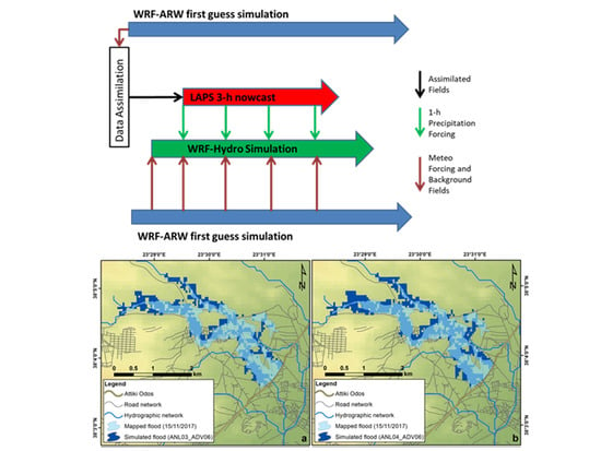
• LAPS used the output fields from the atmospheric component (WRF-ARW) of CHAOS, namely surface and model levels fields of u-, v- components of wind, temperature, relative humidity and 1 h accumulated precipitation as background data (first-guess). Additionally, all available measurements were assimilated into the system (as presented in Section 3), with the most important being the XPOL radar data when available. LAPS ran every hour from 14 November at 14:00 UTC up to 15 November at 06:00 UTC, and produced analysis fields, as well as advected 1 h accumulated precipitation fields for a 3 h forecasting horizon.
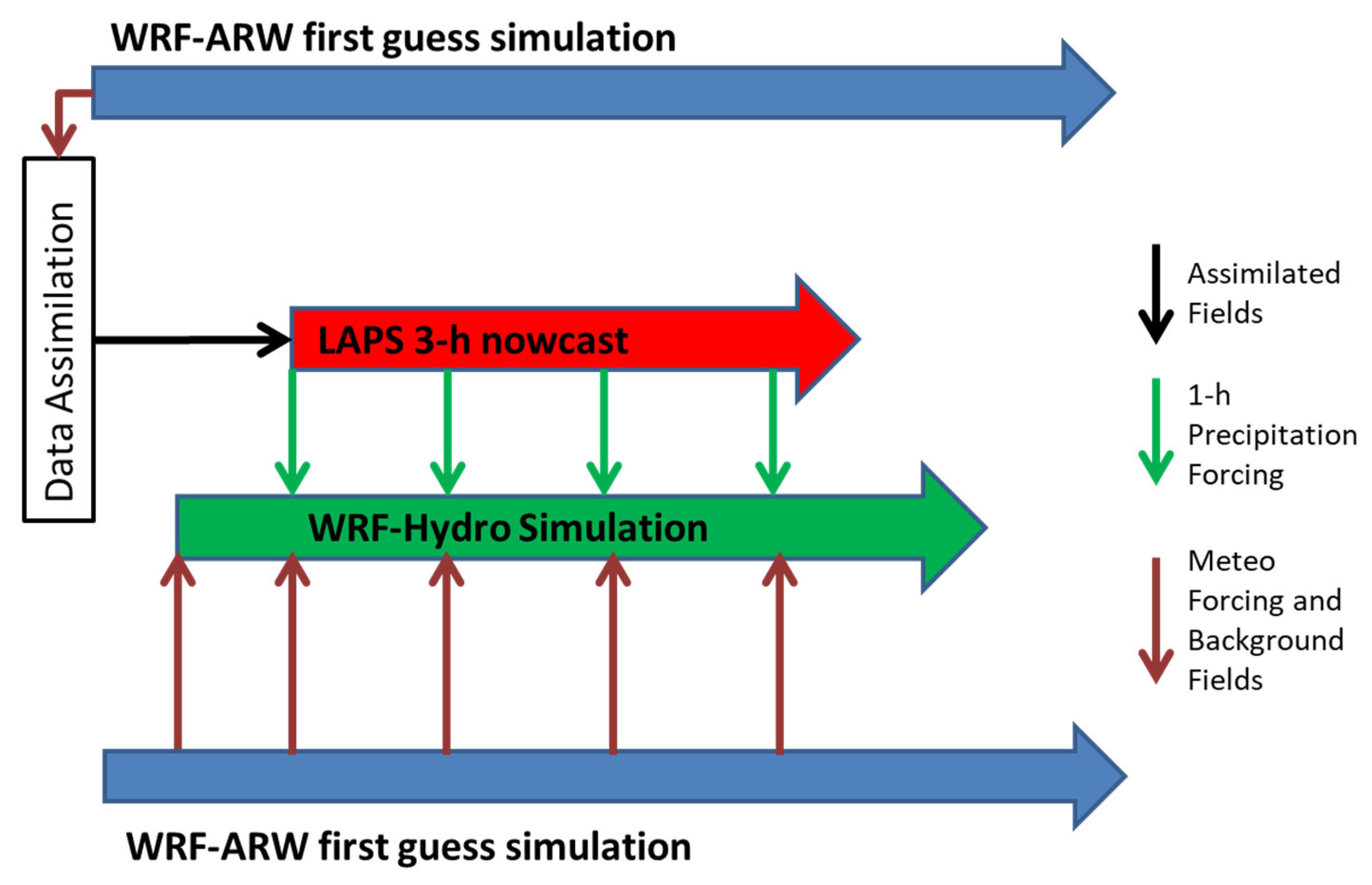
• These precipitation fields were then fed into the hydrological component (WRF-Hydro) of CHAOS, which estimated the streamflow discharge, in order to potentially estimate the stream channels that were most susceptible to extreme flooding. WRF-Hydro was forced by LAPS to run for a 1-h analysis period and a 3-h forecasting horizon (4 h in total), applying cycling and preserving the hydrological properties in the consecutive simulations. Therefore, WRF-Hydro ran every hour from 14 November at 13:00 UTC up to 15 November at 05:00 UTC, i.e., 1 h before the LAPS analyses, to capture the estimation of 1 h accumulated precipitation analyses before the 3 h forecasts. The process was described schematically in Figure 4. WRF-Hydro simulations were performed according to the setup described in Section 3.3. As described in Varlas et al. [36], WRF-Hydro demands various forcing fields, i.e., liquid water precipitation rate, air temperature, and specific humidity at 2 m, incoming shortwave and longwave radiation, u- and v-components of wind at 10 m, and surface pressure.

5. Results and Evaluation

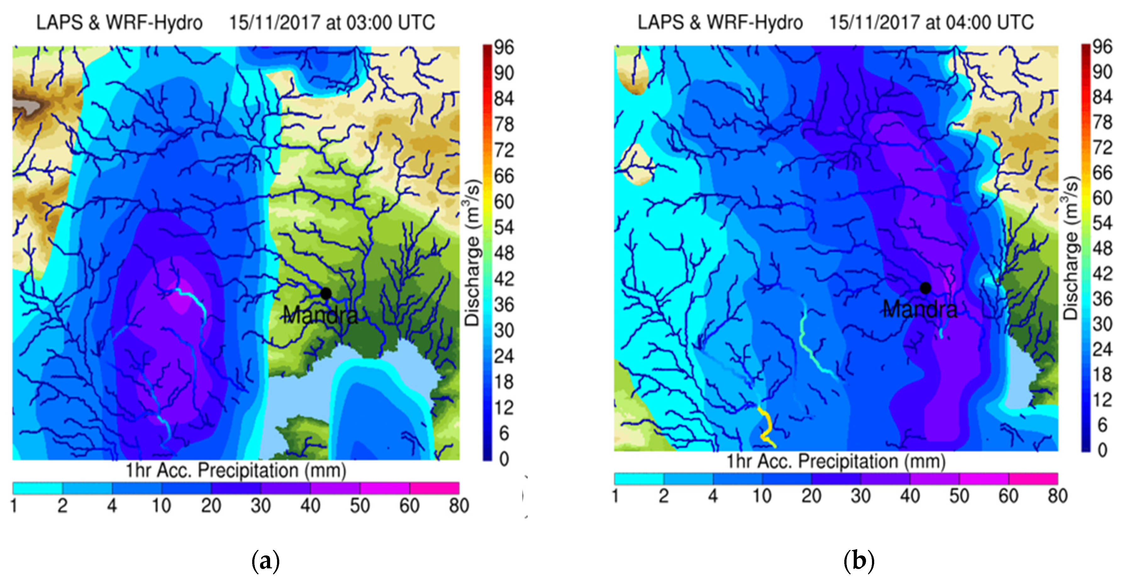
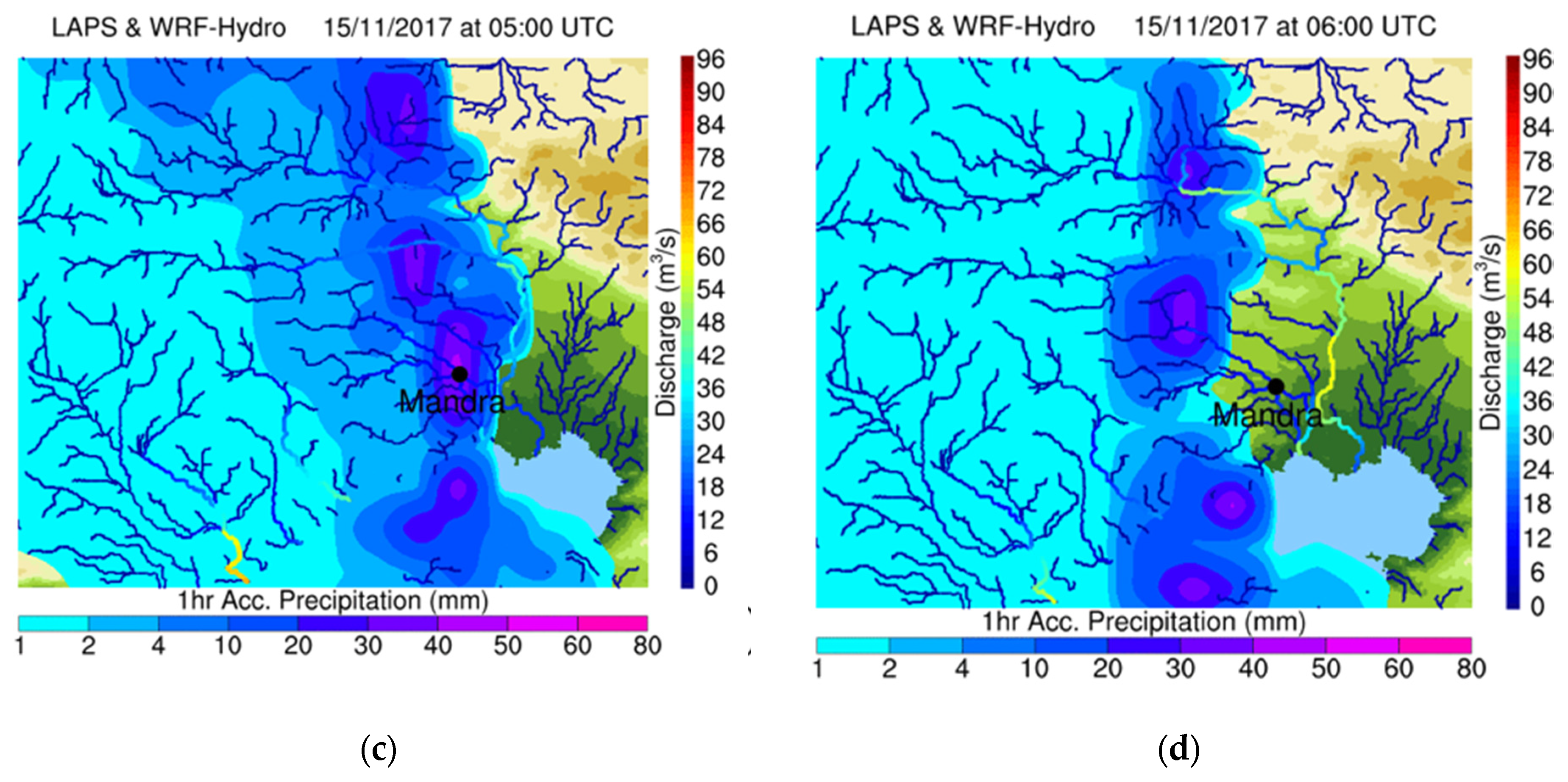
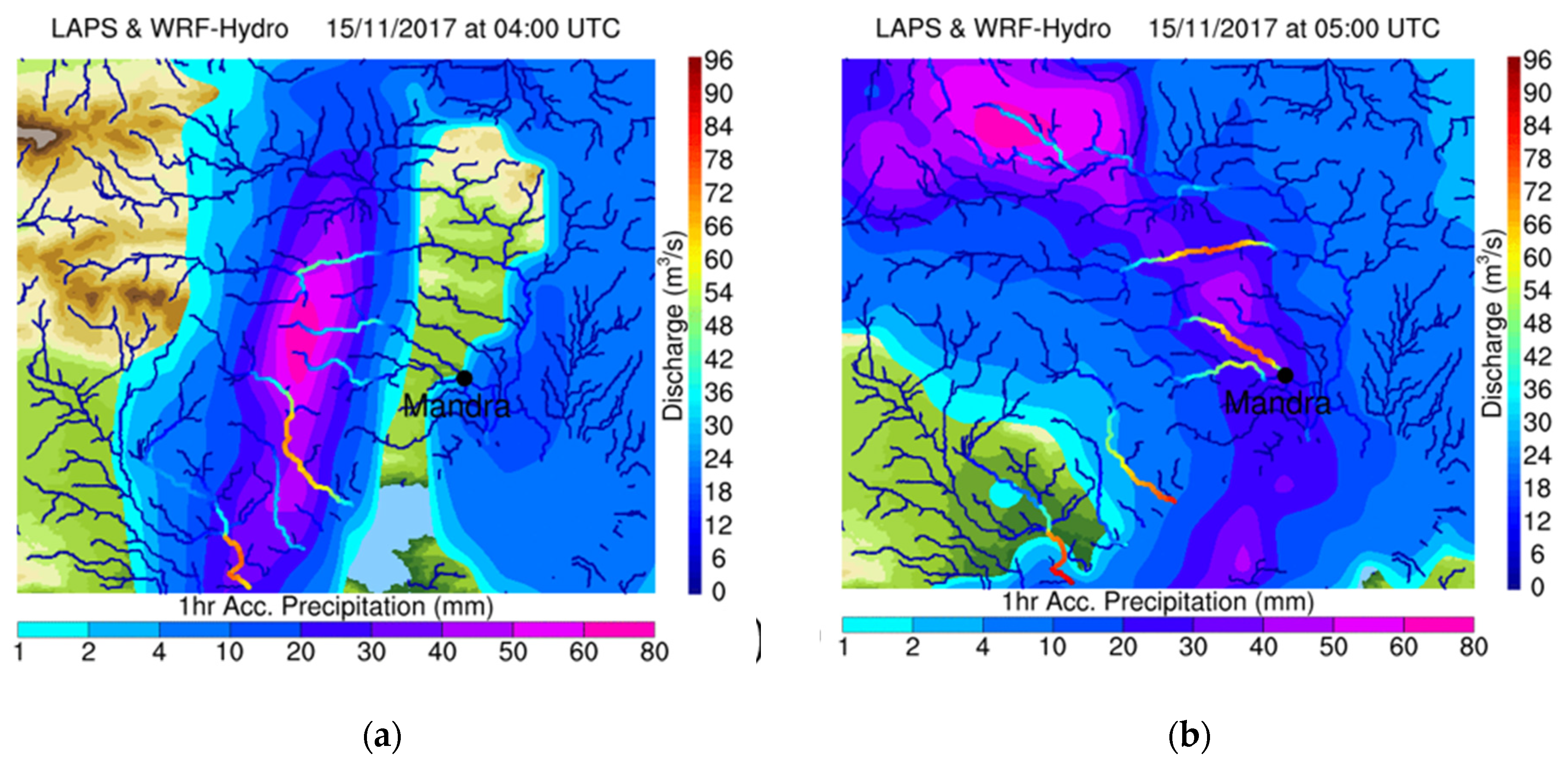
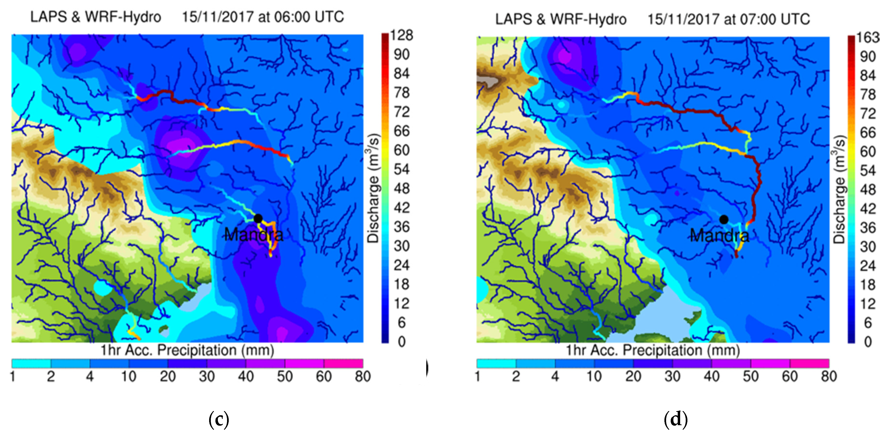
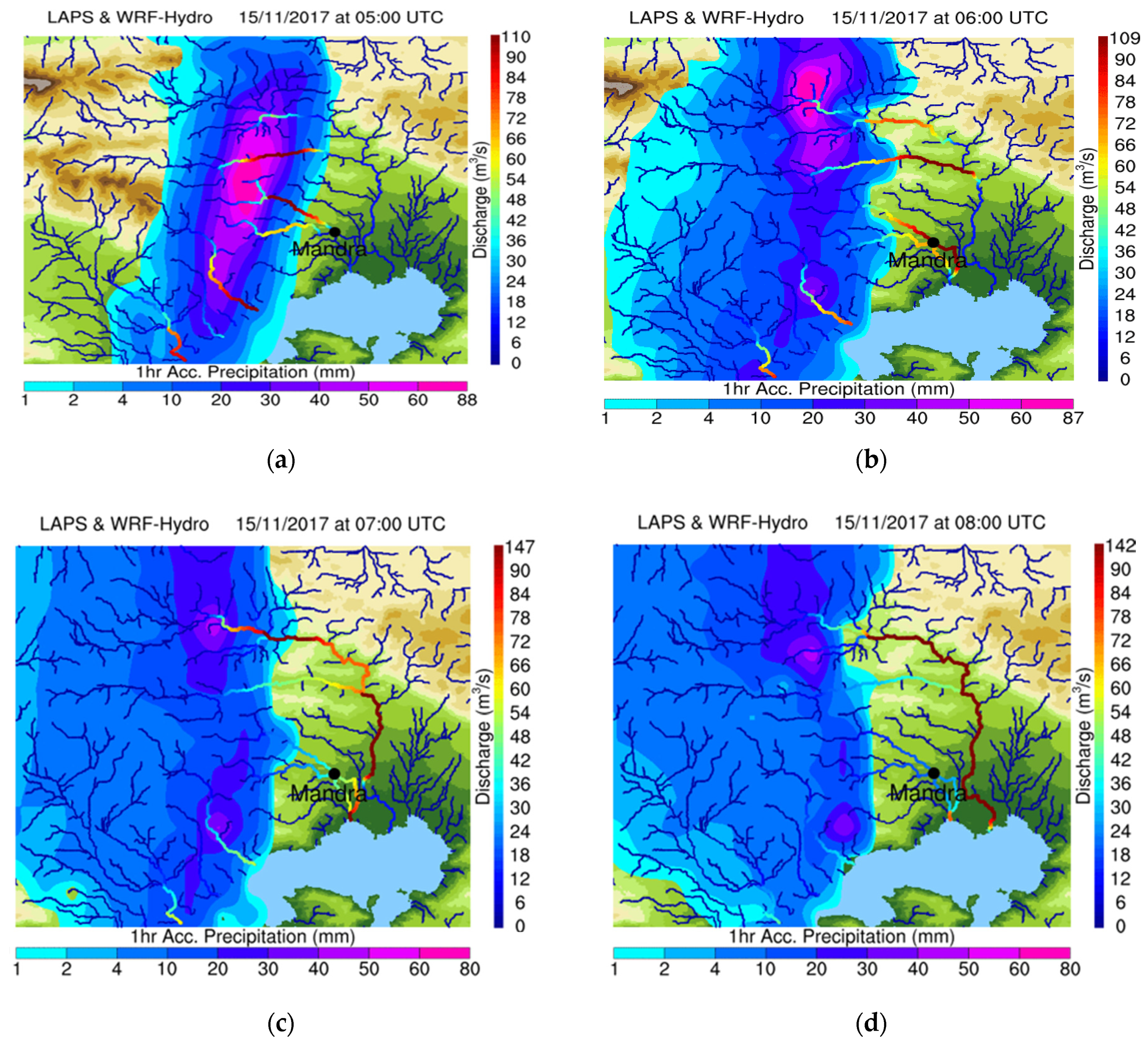
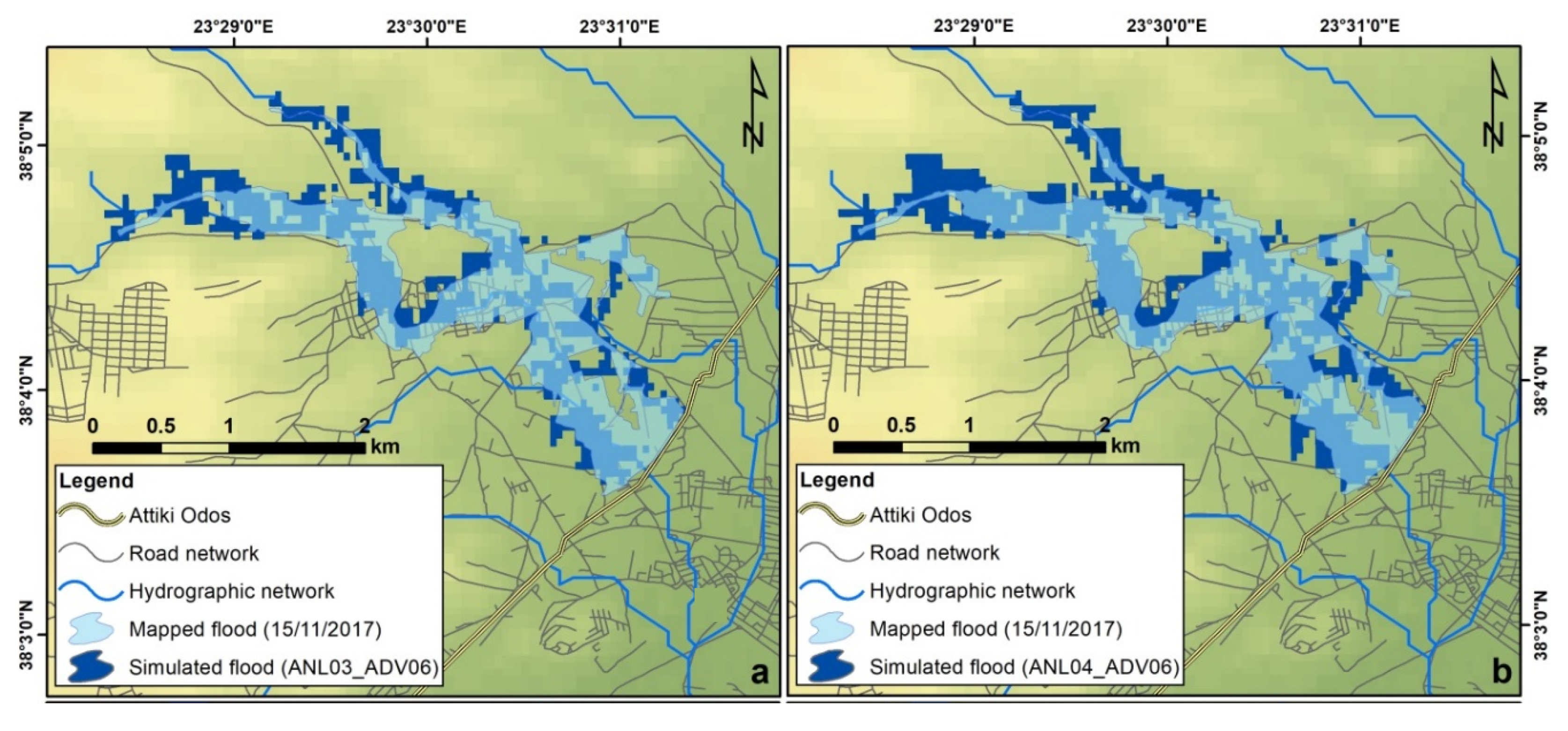
5.1. Nowcasting of Precipitation and Discharge

The most important aspect of an early warning system is to provide reliable alarms, well in advance, in order to give time to the local population and civil authorities to prepare. The simulations closest to the event were evaluated in this regard. The results of the hydrometeorological simulations are presented below in Figure 5, Figure 6 and Figure 7. In each Figure, the simulated discharge by the WRF-Hydro was superimposed to the 1 h accumulated precipitation for each nowcast cycle. More specifically, in Figure 5a–d, WRF-Hydro started on 15 November at 02:00 UTC, with a 4-h forecast window up to 06:00 UTC on hourly output increment, using hourly accumulated precipitation forcing from the LAPS advected fields, valid for 03:00 to 06:00 UTC. WRF-Hydro started one hour before because LAPS provides hourly accumulations starting from the previous hour (02:00 UTC in this case). Similarly, Figure 6 and Figure 7 present the results of the WRF-Hydro simulations, starting on 15 November 03:00 and 04:00 UTC, going up to 07:00 and 08:00 UTC, and using LAPS advected fields from 04:00 to 07:00 UTC and from 05:00 to 08:00 UTC, respectively. The main finding unraveled from analyzing Figure 5 was the dependence of Mandra’s flash flood to very short-scale local rainfall characteristics. Due to the limited extent of Agia Aikaterini and Soures drainage basins, these were prone to flash flooding under heavy rainfall conditions. As Figure 5a depicts, the LAPS analysis for the accumulated precipitation from 02:00 to 03:00 UTC indicated heavy rainfall at the southern slopes of the Pateras Mountain. LAPS advected fields increased precipitation at the basins but the quantity was not enough to cause significant runoff (Figure 5b–d). This happened because the advection routine did not include advanced physics parameterizations or topographic effects on rain and, therefore, could not fully resolve the phenomenon. Nevertheless, streams close to the Nea Peramos and Sarantapotamos stream at the east of Mandra reach discharge values of 60–65 m³/s, indicating the potential of severe phenomena in the region afterwards. In Figure 6a, LAPS analysis for precipitation from 03:00 to 04:00 UTC is shown and it is apparent that the new data assimilated (mostly from the XPOL radar), positions the bulk of the rain again at the south-east slopes of the Pateras Mountain, while increasing in intensity. For the next hours (Figure 6b–d), the core precipitation remains over Mandra, allowing for more water inside the streams, reaching a maximum discharge of 80–90 m³/s in the Soures stream and 50–60 m³/s in the Agia Aikaterini stream, at the time of the flood (05:00–06:00 UTC), while locally exceeding 150 m³/s in the Sarantapotamos stream at 07:00 UTC. This was a clear indication that the streams exceeded a critical soil saturation level and they were probably going to flood. At this time, the system was able to provide a very clear prediction, two h prior to the flooding event, which is considered to be a significant time window for preparedness. Figure 7a–d also verified this effect one hour before the event. In Figure 7a, the amount of rain increased even more at 05:00 UTC and this led to significant discharges of 100–110 m³/s in the Soures stream and 70–75 m³/s in the Agia Aikaterini stream, at the time of the flood. Again, the update of the simulations with the assimilated radar data improved the initial precipitation description and led to an improved simulation of the evolution of the phenomenon.

5.2. Evaluation

For evaluation, since the streams in the area were not routinely monitored, satellite remotesensing images were used from the group of the FloodHub service of BEYOND (Building a Centre of Excellence for Earth Observation based monitoring of Natural Disasters). The simulated flood extent was delineated using the peak water level along the streams [67]. The process was the same as that applied in Varlas et al. [36], in order to maintain consistency with this work and examine the benefits of the methodology used here. Using the discharge and water level (not shown) results from three LAPS nowcast cycles at 02:00, 03:00, and 04:00 UTC, a comparison was made for 06:00 UTC, when the flood presented its peak, against the observed flood extent, taken from the FloodHUB service of BEYOND. Figure 8a demonstrates the results for 06:00 UTC of the WRF-Hydro simulation (dubbed ANL03_ADV06), starting on 15 November at 02:00 UTC and using LAPS nowcasts from 03:00 to 06:00 UTC. In the same way, Figure 8b,c show the results of the WRF-Hydro simulations (dubbed ANL04_ADV06 and dubbed ANL05_ADV06) for 06:00 UTC. The latter simulations start on 15 November at 03:00 and 04:00 UTC and use LAPS nowcasts for the periods 04:00–07:00 UTC and 05:00–08:00 UTC, respectively. For comparison, the hindcasting WRF-Hydro flood simulation with the XPOL radar data, as shown in Varlas et al. ([36]; dubbed RAD06) is also illustrated (Figure 8b). It should be noted that the evaluation was restricted to the area upstream of the “Attiki Odos” highway and only the sixth-order streams were used (Figure 8a–d).

Since flood events can be treated as categorical forecasts [68], they can be evaluated using contingency tables (

Table 2. Contingency table for validation and statistical scores definitions, based on the contingency table.

		Yes	No	PoD = a/(a + c)
		Observed event		FAR = b/(a + b)
Yes	Simulated event	Hit (a)	False alarm (b)	CSI = a/(a + b + c)
No		Miss (c)	Correct non-event (d)	B = (a + b)/(a + c)

), which sum up all possible combinations of forecast and observed events [69]. The combination of verification measures and scores associated with the contingency table used for the evaluation of forecasts in the present study were—probability of detection (PoD), false alarm ratio (FAR), critical success index (CSI), and the frequency bias (B) [70].

The probability of detection (PoD or hit rate HR) ranged between 0 and 1, with 0 representing failure in forecasting and 1 representing a perfect forecast. PoD is sensitive only to missed events and not false alarms, and therefore, it is incomplete by itself [71] and can be used in relation to the false alarm ratio (FAR) as pairs of sufficient statistics [72]. FAR ranges between 0 and 1, with 0 representing a perfect forecast and 1 representing a failure of forecast. This score was not sensitive to missed events and it was also an incomplete score and should be used in pairs with the PoD. The Critical Success Index (CSI or threat score TS) ranged between 0 and 1, with 0 representing failure in forecasting, and 1 representing a perfect forecast. CSI was sensitive to both missed events and false alarms, but was affected by the climatological frequency of the event. Nevertheless, for evaluation of a forecast or for comparison of the accuracy of forecasts, based on the same dataset, CSI was considered to be sufficient [70]. The frequency bias (B) was not an actual verification score, since it only compared the forecast and observed frequencies of occurrence of the event in the sample. B values of 1 represented the best score, values higher than 1 indicated overestimation, and values less than 1 indicated underestimation [70].

The above statistical scores were calculated using the data from the three simulations and the FloodHUB service, and they are presented in

Table 3. Statistical indices for all WRF-Hydro simulations, using input data from LAPS-advected fields. The time of the peak flood, i.e., 06:00 UTC, was noted using the yellow color. Additionally, the comparison with the XPOL radar data presented in the bottom row was made as reference, facilitating the assessment of the results.

Starting Date	Forecast Hour	PoD	CSI	FAR	B
15/11 at 03:00 ANL03_ADV06	+0 h	0.46	0.35	0.42	0.79
	+1 h	0.45	0.34	0.42	0.77
	+2 h	0.48	0.35	0.42	0.82
	+3 h	0.49	0.36	0.41	0.83
15/11 at 04:00 ANL04_ADV06	+0 h	0.43	0.33	0.42	0.74
	+1 h	0.51	0.36	0.45	0.93
	+2 h	0.61	0.42	0.42	1.05
	+3 h	0.53	0.39	0.41	0.90
15/11 at 05:00 ANL05_ADV06	+0 h	0.48	0.34	0.46	0.89
	+1 h	0.67	0.45	0.43	1.16
	+2 h	0.58	0.41	0.42	1.00
	+3 h	0.53	0.38	0.42	0.90
CHAOS	-	0.43	0.33	0.43	0.75
Radar Data 15/11 at 06:00 RAD06	+0 h	0.68	0.45	0.43	1.18

. As a point of reference, the same scores were calculated from the WRF-Hydro simulation, using only the XPOL radar data (as also presented in [36]). In each column, the PoD, CSI, FAR, and B were calculated for different starting hours and for the 3 h short-term forecasts. In the table, the yellow color denoted the time of the peak flood, namely 15 November 2017 at 06:00 UTC.

The comparison of the results of the three hydrological simulations showed that 3 h before the flood, the system had a PoD of 0.49, a CSI of 0.26, a FAR of 0.41, and a B of 0.83. These results indicated a blurry prediction of the intense flash flood, 3 h before, but they became better, the closer we got to the event. Thus, one hour before the peak flood at 06:00 UTC, the statistical indices were comparable to those of the XPOL radar, reaching a PoD of 0.67, a CSI of 0.45, a FAR of 0.43, and a B of 1.16. This was an encouraging finding because it seemed that one hour before the peak of the flood, we could have a flash flood warning with reliable accuracy. Even 2 h before the event, there was a 61% probability of detection (CSI of 0.42, FAR of 0.42, and B of 1.05), a sufficient result to be used for early warning. In comparison, Varlas et al. [36] reported values of a PoD of 0.43, a CSI of 0.33, a FAR of 0.43, and a B of 0.75 for the WRF-Hydro, driven solely from WRF-ARW’s results; the same was used in this study as the background fields of the LAPS model. These values were considerably worse than the ones from the WRF-Hydro driven by LAPS advections, which was to be expected due to two factors—(1) there was no data assimilation (especially the radar data) in the WRF-ARW simulation for this case, and (2) the short-term forecasting horizon fell into the model spin-up time, thus, diminishing the forecasting accuracy. This was another indication of the added benefits from the methodology used here, in contrast to typical forecasting operations that were used as a basis for early-warning systems, namely a lone regional model (albeit a very advanced and reliable one, as was WRF-ARW).

The statistical analysis revealed that the developed system was highly accurate, 1 and 2 h before the event, and gave an acceptable prognostic signal, even 3 h before the flood. Therefore, in an operation-like mode (running continuously on hourly cycle), the system would be able to notify the proper authorities, well in advance of the devastating flood, potentially 2 to 3 h ahead. It is important to note that even a 2 h “head start” on the local authorities could have saved the people that died or were injured, during this event. These nowcasts (1–3 h forecasts) could support operational short-term forecasts (3–5 days) and medium-range forecasts (10–15 days), as a part of a wider early warning system for hydrometeorological hazards. The added benefit of the system was that it demanded very little computational power, making it possible to continuously provide results every hour, without the need for an HPC, which is usually essential for proper regional model setups. For reference, it is possible to run the system in a typical desktop PC or laptop, and it takes, at the most, a 20–30 min of runtime. The preparation of alarms and warnings was also fast, keeping everything well under an hour. Finally, automating the data conversion and flow from the radar to the system was very fast and no severe delays were expected, since it could be done in a few minutes.

6. Conclusions

In this study, a hydrometeorological nowcasting methodology was implemented as an early warning system in a case study of an extreme flash flood event. The system was based on the combination of a series of in-situ and remotesensing measurements, a data assimilation model, namely LAPS, and the hydrological component of the “state-of-the-art” CHAOS modeling system. The LAPS assimilation system was upgraded with the capability to use high-resolution background fields, provided by WRF-ARW, as well as to advect the assimilated precipitation fields and, then, to feed the WRF-Hydro component for flood prediction in short-time scales of 1 to 3 h, in advance. The methodology used here attempted to combine all common practices for nowcasting, which usually involved either data assimilation methodologies or high-resolution numerical models (as presented in the introduction), with the addition of a hydrological component for proper water flow representation and ultimately accurate flood warnings.

To test the system, the devastating flash flood event in the Mandra town, Western Attica, Greece, on 15 November 2017 was selected, due to the severity of the phenomenon and the resulting 24 fatalities that were recorded. The combined system used a vast number of actual data for assimilation (METARS, SYNOP, RAOB, GPM, etc.) and most importantly accumulated precipitation estimations from the XPOL weather radar operated by the National Observatory of Athens. The resulting fields were advected using the methodology described in Section 3.1 and the outputs were used as input for WRF-Hydro, which provided flood discharge and water level, in order to approximate flood extent. The discharge values provided a clear indication of the severity of the flooding event 3 h beforehand, with the simulations 2 h before solidifying that the Agia Aikaterini and the Soures streams near Mandra were going to overflow and action was needed. Simulations one hour before the event verified this. Using satellite data from the FloodHUB service, several statistical indices were calculated in order to establish the accuracy of the system. It was found that the developed system could have provided reliable early warning of the flood event up to 3 h in advance, giving vital time to the local authorities to mobilize and even prevent fatalities and injuries to the local population. The closest to the event nowcast cycle, at 05:00 UTC, showed a PoD of 0.67, a CSI of 0.45, a FAR of 0.45, and a B of 1.16 of its hourly precipitation forecast. These scores were comparable to the relevant statistical indices of the recorded precipitation from the XPOL weather radar, at 06:00 UTC.

Due to the nature of the system, it demanded little in terms of computing power (in contrast to high-resolution numerical models) to provide good results, making it easy to operate constantly and provide reliable nowcasts every hour. Another benefit was the flexibility of the model, since it can provide nowcasts with any number of available data. This was a simulation using all available data “post-case”. In real-time applications, several of these data sources would not be available for use when needed. However, the most important precipitation information source was the radar data, which could be used in real time. Additionally, the system had the added capability to incorporate real-time data from systems installed specifically to support the simulations (for example, weather stations deployed at high-risk areas, which would feed data in real-time). In addition, even if the radar system (which represents the best possible representation of rain) was not operational, LAPS and WRF-Hydro, together with background fields from WRF-ARW, would still provide early warnings, albeit not the best possible ones.

Therefore, the developed system could be used as an early warning system or as a component of an advanced early warning system for hydrometeorological hazards. However, even though the scientific basis behind this work was sound, more testing is required in high-impact phenomena to fully examine the capabilities of the system. This work is the first step where we present the development of the system and the robustness of our methodology in a severe case. This process could also be a useful learning tool in a broad spectrum of scientific areas, beyond atmospheric research or even academia. In addition, it should be noted that flood management requires not only reliable forecasts at various timescales, but also trained forecasters, engaging water management agencies, and local or municipal authorities, along with transport and communications operations and emergency services.

References

1. Seneviratne, S.; Nicholls, N.; Easterling, D.; Goodess, C.; Kanae, S.; Kossin, J.; Luo, Y.; Marengo, J.; McInnes, K.; Rahimi, M.; et al. Changes in climate extremes and their impacts on the natural physical environment. In Managing the Risks of Extreme Events and Disasters to Advance Climate Change Adaptation; Barros, C.B.V., Stocker, T.F., Qin, D., Dokken, D.J., Ebi, K.L., Mastrandrea, M.D., Mach, K.J., Plattner, G.-K., Allen, S.K., Tignor, M., et al., Eds.; A Special Report of Working Groups I and II of the Intergovernmental Panel on Climate Change (IPCC); Cambridge University Press: Cambridge, UK; New York, NY, USA, 2012; pp. 109–230. [Google Scholar]
2. Collins, M.; Sutherland, M.; Bouwer, L.; Cheong, S.-M.; Frölicher, T.; Jacot Des Combes, H.; Koll Roxy, M.; Losada, I.; McInnes, K.; Ratter, B.; et al. Extremes, Abrupt Changes and Managing Risk. In IPCC Special Report on the Ocean and Cryosphere in a Changing Climate; Pörtner, H.-O., Roberts, D.C., Masson-Delmotte, V., Zhai, P., Tignor, M., Poloczanska, E., Mintenbeck, K., Alegría, A., Nicolai, M., Okem, A., et al., Eds.; 2019; in press. [Google Scholar]
3. Smith, A.B.; Katz, R.W. US billion-dollar weather and climate disasters: Data sources, trends, accuracy and biases. Nat. Hazards 2013, 67, 387–410. [Google Scholar] [CrossRef]
4. Hirabayashi, Y.; Mahendran, R.; Koirala, S.; Konoshima, L.; Yamazaki, D.; Watanabe, S.; Kim, H.; Kanae, S. Global flood risk under climate change. Nat. Clim. Chang. 2013, 3, 816–821. [Google Scholar] [CrossRef]
5. CRED. Natural Disasters. Available online: https://www.cred.be/sites/default/files/CREDNaturalDisaster2018.pdf (accessed on 25 June 2020).
6. Meehl, G.A.; Arblaster, J.M.; Tebaldi, C. Understanding future patterns of precipitation extremes in climate model simulations. Geophys. Res. Lett. 2005, 32, L18719. [Google Scholar] [CrossRef] [Green Version]
7. Mentzafou, A.; Varlas, G.; Dimitriou, E.; Papadopoulos, A.; Pytharoulis, I.; Katsafados, P. Modeling the Effects of Anthropogenic Land Cover Changes to the Main Hydrometeorological Factors in a Regional Watershed, Central Greece. Climate 2019, 7, 129. [Google Scholar] [CrossRef] [Green Version]
8. UNISDR. Early Warning Practices Can Save Many Lives: Good Practices and Lessons Learned; UNISDR: Bonn, Germany, 2010; pp. 1–67. [Google Scholar]
9. Wilson, J.W.; Crook, N.A.; Mueller, C.K.; Sun, J.; Dixon, M. Nowcasting thunderstorms: A status report. Bull. Am. Meteorol. Soc. 1998, 79, 2079–2100. [Google Scholar] [CrossRef]
10. Wilson, J.W.; Ebert, E.E.; Saxen, T.R.; Roberts, R.D.; Mueller, C.K.; Sleigh, M.; Pierce, C.E.; Seed, A. Sydney 2000 forecast demonstration project: Convective storm nowcasting. Weather Forecasting. 2004, 19, 131–150. [Google Scholar] [CrossRef]
11. Liguori, S.; Rico-Ramirez, M.A. Quantitative assessment of short-term rainfall forecasts from radar nowcasts and MM5 forecasts. Hydrol. Process. 2012, 26, 3842–3857. [Google Scholar] [CrossRef]
12. Liu, Z.; Dai, Q.; Zhuo, L. Relationship between Rainfall Variability and the Predictability of Radar Rainfall Nowcasting Models. Atmosphere 2019, 10, 458. [Google Scholar] [CrossRef] [Green Version]
13. Wang, Y.; Meirold-Mautner, I.; Kann, A.; Slak, A.Š.; Simon, A.; Vivoda, J.; Bica, B.; Böcskör, E.; Brezková, L.; Dantinger, J.; et al. Integrating nowcasting with crisis management and risk prevention in a transnational and interdisciplinary framework. Meteorol. Z. 2017, 26, 459–473. [Google Scholar] [CrossRef]
14. Wapler, K.; Bañón Peregrín, L.M.; Buzzi, M.; Heizenreder, D.; Kann, A.; Meirold-Mautner, I.; Simon, A.; Wang, Y. Conference Report 2nd European Nowcasting Conference. Meteorol. Z. 2018, 27, 81–84. [Google Scholar] [CrossRef]
15. Pulkkinen, S.; Chandrasekar, V.; Harri, A.M. Fully Spectral Method for Radar-Based Precipitation Nowcasting. J. Sel. Top. Appl. Earth Obs. Remote Sens. 2019, 12, 1369–1382. [Google Scholar] [CrossRef]
16. Huang, L.X.; Isaac, G.A.; Sheng, G. Integrating NWP Forecasts and Observation Data to Improve Nowcasting Accuracy. Weather Forecast. 2012, 27, 938–953. [Google Scholar] [CrossRef]
17. Browning, K.; Collier, C.; Larke, P.; Menmuir, P.; Monk, G.; Owens, R. On the Forecasting of Frontal Rain Using a Weather Radar Network. Mon. Weather Rev. 1982, 110, 534–552. [Google Scholar] [CrossRef] [Green Version]
18. Benjamin, S.G.; Dévényi, D.; Weygandt, S.S.; Brundage, K.J.; Brown, J.M.; Grell, G.A.; Kim, D.; Schwartz, B.E.; Smirnova, T.G.; Smith, T.L.; et al. An Hourly Assimilation–Forecast Cycle: The RUC. Mon. Weather Rev. 2004, 132, 495–518. [Google Scholar] [CrossRef]
19. Mass, C. Nowcasting: The Promise of New Technologies of Communication, Modeling, and Observation. Bull. Am. Meteorol. Soc. 2012, 93, 797–809. [Google Scholar] [CrossRef] [Green Version]
20. Pierce, C.; Ebert, E.; Seed, A.; Sleigh, M.; Collier, C.; Fox, N.; Donaldson, N.; Wilson, J.W.; Roberts, R.; Mueller, C.K. The Nowcasting of Precipitation during Sydney 2000: An Appraisal of the QPF Algorithms. Weather Forecast. 2004, 19, 7–21. [Google Scholar] [CrossRef]
21. Wilson, J.; Feng, Y.; Chen, M.; Roberts, R. Nowcasting Challenges during the Beijing Olympics: Successes, Failures, and Implications for Future Nowcasting Systems. Weather Forecast. 2010, 25, 1691–1714. [Google Scholar] [CrossRef]
22. Miyoshi, T.; Kondo, K.; Terasaki, K. Big Ensemble Data Assimilation in Numerical Weather Prediction. Computer 2015, 48, 15–21. [Google Scholar] [CrossRef]
23. Kalnay, E. Atmospheric Modeling, Data Assimilation and Predictability; Cambridge University Press: Cambridge, UK, 2003. [Google Scholar]
24. Khare, S.P.; Anderson, J.L. An examination of ensemble filter based adaptive observation methodologies. Tellus A 2006, 58, 179–195. [Google Scholar] [CrossRef]
25. Zhang, F.; Snyder, C.; Sun, J. Impacts of initial estimate and observation availability on convective-scale data Assimilation with an Ensemble Kalman Filter. Mon. Weather Rev. 2004, 132, 1238–1253. [Google Scholar] [CrossRef]
26. Dixon, M.; Wiener, G. TITAN: Thunderstorm Identification, Tracking, Analysis, and Nowcasting—A Radar-based Methodology. J. Atmos. Oceanic Technol. 1993, 10, 785–797. [Google Scholar] [CrossRef]
27. Ruzanski, E.; Chandrasekar, V.; Wang, Y. The CASA nowcasting system. Journal of Atmospheric and Oceanic Technology. J. Atm. Ocean Technol. 2011, 28, 640–655. [Google Scholar] [CrossRef]
28. Haiden, T.; Kann, A.; Wittmann, C.; Pistotnik, G.; Bica, B.; Gruber, C. The Integrated Nowcasting through Comprehensive Analysis (INCA) System and Its Validation over the Eastern Alpine Region. Weather Forecast. 2011, 26, 166–183. [Google Scholar] [CrossRef]
29. Bowler, N.E.; Pierce, C.E.; Seed, A.W. STEPS: A probabilistic precipitation forecasting scheme which merges an extrapolation nowcast with downscaled NWP. Q. J. R. Meteorol. Soc. 2006, 132, 2127–2155. [Google Scholar] [CrossRef]
30. Seed, A.W.; Pierce, C.E.; Norman, K. Formulation and evaluation of a scale decomposition-based stochastic precipitation nowcast scheme. Wat. Resour. Res. 2013, 49, 6624–6641. [Google Scholar] [CrossRef]
31. Auger, L.; Dupont, O.; Hagelin, S.; Brousseau, P.; Brovelli, P. AROME–NWC: A new nowcasting tool based on an operational mesoscale forecasting system. Q. J. Roy. Meteor. Soc. 2015, 141, 1603–1611. [Google Scholar] [CrossRef]
32. Albers, S. The LAPS wind analysis. Weather Forecast. 1995, 10, 342–352. [Google Scholar] [CrossRef] [Green Version]
33. Albers, S.C.; Mcginley, J.A.; Birkenheuer, D.L.; Smart, J.R. The Local Analysis and Prediction System (LAPS): Analyses of Clouds, Precipitation, and Temperature. Weather Forecast. 1996, 11, 273–287. [Google Scholar] [CrossRef] [Green Version]
34. Varlas, G. Development of an Integrated Modeling System for Simulating the Air-Ocean Wave Interactions. Ph.D. Thesis, Harokopio University of Athens (HUA), Athens, Greece, 2017. Available online: https://www.didaktorika.gr/eadd/handle/10442/41238 (accessed on 21 April 2020).
35. Varlas, G.; Katsafados, P.; Papadopoulos, A.; Korres, G. Implementation of a two-way coupled atmosphere-ocean wave modeling system for assessing air-sea interaction over the Mediterranean Sea. Atmos. Res. 2018, 208, 201–217. [Google Scholar] [CrossRef]
36. Varlas, G.; Anagnostou, M.; Spyrou, C.; Papadopoulos, A.; Kalogiros, J.; Mentzafou, A.; Michaelides, S.; Baltas, E.; Karymbalis, E.; Katsafados, P. A Multi-Platform Hydrometeorological Analysis of the Flash Flood Event of 15 November 2017 in Attica, Greece. Remote Sens. 2019, 11, 45. [Google Scholar] [CrossRef] [Green Version]
37. Varlas, G.; Spyrou, C.; Papadopoulos, A.; Korres, G.; Katsafados, P. One-year assessment of the CHAOS two-way coupled atmosphere-ocean wave modelling system over the Mediterranean and Black Seas. Mediter. Mar. Sci. 2020, 21, 372–385. [Google Scholar] [CrossRef]
38. Katsafados, P.; Varlas, G.; Papadopoulos, A.; Spyrou, C.; Korres, G. Assessing the implicit rain impact on sea state during hurricane Sandy (2012). Geophys. Res. Lett. 2018, 45, 12015–12022. [Google Scholar] [CrossRef]
39. Skamarock, W.C.; Klemp, J.B.; Dudhia, J.; Gill, D.O.; Liu, Z.; Berner, J.; Wang, W.; Powers, J.G.; Duda, M.G.; Barker, D.M.; et al. A Description of the Advanced Research WRF Version 4; NCAR Technical Note NCAR/TN-556+STR; NCAR: Boulder, CO, USA, 2019. [Google Scholar] [CrossRef]
40. Powers, J.G.; Klemp, J.B.; Skamarock, W.C.; Davis, C.A.; Dudhia, J.; Gill, D.O.; Coen, J.L.; Gochis, D.J.; Ahmadov, R.; Peckham, S.E.; et al. The Weather Research and Forecasting Model: Overview, System Efforts, and Future Directions. Bull. Am. Meteor. Soc. 2017, 98, 1717–1737. [Google Scholar] [CrossRef]
41. Gochis, D.J.; Yu, W.; Yates, D.N. The WRF-Hydro Model Technical Description and User’s Guide, Version 3.0; NCAR Technical Document; NCAR: Boulder, CO, USA, 2015; Available online: https://ral.ucar.edu/sites/default/files/public/images/project/WRF_Hydro_User_Guide_v3.0.pdf (accessed on 25 June 2020).
42. Diakakis, M.; Andreadakis, E.; Nikolopoulos, E.I.; Spyrou, N.I.; Gogou, M.E.; Deligiannakis, G.; Katsetsiadou, N.K.; Antoniadis, Z.; Melaki, M.; Georgakopoulos, A.; et al. An integrated approach of ground and aerial observations in flash flood disaster investigations. The case of the 2017 Mandra flash flood in Greece. Int. J. Disast. Risk Red. 2019, 33, 290–309. [Google Scholar] [CrossRef]
43. Stamou, A.I. The disastrous flash flood of Mandra in Attica-Greece and now what? Civ. Eng. Res. J. 2018, 6, 1–6. [Google Scholar] [CrossRef] [Green Version]
44. Mavrakis, A.; Theoharatos, G.; Asimakopoulos, D.; Christides, A. Distribution of the trace metals in sediments of Eleusis Gulf. Mediterr. Mar. Sci. 2004, 5, 151–158. [Google Scholar] [CrossRef] [Green Version]
45. Bellos, V.; Papageorgaki, I.; Kourtis, I.; Vangelis, H.; Kalogiros, I.; Tsakiris, G. Reconstruction of a flash flood event using a 2D hydrodynamic model under spatial and temporal variability of storm. Nat. Hazards 2020, 101, 711–726. [Google Scholar] [CrossRef]
46. Alberoni, P.P.; Levizzani, V.; Mezzasalma, P.; Costa, S.; Rizzi, R. Impact of Meteorological Radar and Satellite Data onto Mesoscale Analyses. In Proceedings of the Mediterranean Storms-EGS Plinius Conference, Baja Sardinia, Italy, 16–18 October 2000; pp. 545–556. [Google Scholar]
47. Hiemstra, C.A.; Liston, G.E.; Pielke, R.A., Sr.; Birkenheuer, D.L.; Albers, S. Comparing local analysis and prediction system (LAPS) assimilations with independent observations. Weather Forecast. 2006, 21, 1024–1040. [Google Scholar] [CrossRef]
48. Barnes, S. A Technique for Maximizing Details in Numerical Weather Map Analysis. J. Appl. Meteor. 1964, 3, 396–409. [Google Scholar] [CrossRef] [Green Version]
49. FAO. The Digitized Soil Map of the World, World Soil Resource Rep. 67; FAO: Rome, Italy, 1991. [Google Scholar]
50. Csiszar, I.; Gutman, G. Mapping global land surface albedo from NOAA/AVHRR. J. Geophys. Res. 1999, 104, 6215–6228. [Google Scholar] [CrossRef]
51. Valcke, S.; Craig, T.; Coquart, L. OASIS3-MCT_3.0 Coupler User Guide; CERFACS/CNRS: Toulouse, France, 2015; Available online: http://www.cerfacs.fr/oa4web/oasis3-mct_3.0/oasis3mct_UserGuide.pdf (accessed on 25 June 2020).
52. Craig, A.; Valcke, S.; Coquart, L. Development and performance of a new version of the OASIS coupler, OASIS3-MCT_3.0. Geosci. Model Dev. 2017, 10, 3297–3308. [Google Scholar] [CrossRef] [Green Version]
53. Group, T.W. The WAM model—A third generation ocean wave prediction model. J. Phys. Oceanogr. 1988, 18, 1775–1810. [Google Scholar] [CrossRef] [Green Version]
54. Komen, G.J.; Cavaleri, L.; Donelan, M.; Hasselmann, K.; Hasselmann, S.; Janssen, P.A.E.M. Dynamics and Modelling of Ocean Waves; Cambridge University Press: Cambridge, UK, 1994. [Google Scholar]
55. AWN’s Digital Atmosphere Page. Available online: http://www.australianweathernews.com/digatm/ (accessed on 7 June 2020).
56. NCEP Restricted Data-ACARS and AMDAR. Available online: https://www.nco.ncep.noaa.gov/pmb/docs/restricted_data/acars+amdar/ (accessed on 23 April 2020).
57. Sharifi, E.; Steinacker, R.; Saghafian, B. Assessment of GPM-IMERG and Other Precipitation Products against Gauge Data under Different Topographic and Climatic Conditions in Iran: Preliminary Results. Remote Sens. 2016, 8, 135. [Google Scholar] [CrossRef] [Green Version]
58. Global Precipitation Measurement (GPM) Mission Overview_Precipitation Measurement Missions. Available online: https://pmm.nasa.gov/GPM (accessed on 21 June 2020).
59. Hou, A.Y.; Kakar, R.K.; Neeck, S.; Azarbarzin, A.A.; Kummerow, C.D.; Kojima, M.; Oki, R.; Nakamura, K.; Iguchi, T. The global precipitation measurement mission. Bull. Am. Meteorol. Soc. 2014, 95, 701–722. [Google Scholar] [CrossRef]
60. Huffman, G.J.; Bolvin, D.T.; Nelkin, E.J. Integrated Multi-Satellite Retrievals for GPM (IMERG) Technical Documentation; NASA/GSFC: Greenbelt, MD, USA, 2015. Available online: https://gpm.nasa.gov/sites/default/files/document_files/IMERG_doc.pdf (accessed on 7 June 2020).
61. Tong, K.; Zhao, Y.; Wei, Y.; Hu, B.; Lu, Y. Evaluation and Hydrological Validation of GPM Precipitation Products over the Nanliu River Basin, Beibu Gulf. Water 2018, 10, 1777. [Google Scholar] [CrossRef] [Green Version]
62. Anagnostou, M.N.; Kalogiros, J.; Marzano, F.S.; Anagnostou, E.N.; Montopoli, M.; Picciotti, E. Performance evaluation of a new dual-polarization microphysical algorithm based on long-term X-band radar and disdrometer observations. J. Hydrometeorol. 2013, 14, 560–576. [Google Scholar] [CrossRef]
63. Kalogiros, J.; Anagnostou, M.N.; Anagnostou, E.N.; Montopoli, M.; Picciotti, E.; Marzano, F.S. Evaluation of a new polarimetric algorithm for rain-path attenuation correction of X-band radar observations against disdrometer. IEEE Trans. Geosci. Remote Sens. 2014, 52, 1369–1380. [Google Scholar] [CrossRef]
64. Lehner, B.; Verdin, K.; Jarvis, A. New Global Hydrography Derived from Spaceborne Elevation Data. EOS Trans. Am. Geophys. Union. 2008, 89, 93–94. [Google Scholar] [CrossRef]
65. Jarvis, A.; Reuter, H.I.; Nelson, A.; Guevara, E. Hole-Filled SRTM for the Globe Version 4. CGIAR-CSI SRTM 90 m Database. Available online: http://srtm.csi.cgiar.org (accessed on 21 April 2020).
66. Papaioannou, G.; Varlas, G.; Terti, G.; Papadopoulos, A.; Loukas, A.; Panagopoulos, Y.; Dimitriou, E. Flood Inundation Mapping at Ungauged Basins Using Coupled Hydrometeorological–Hydraulic Modelling: The Catastrophic Case of the 2006 Flash Flood in Volos City, Greece. Water 2019, 11, 2328. [Google Scholar] [CrossRef] [Green Version]
67. FloodHub. Analysis of the Flood in Western Attica on 15/11/2017 Using Satellite Remote Sensing. 2018. Available online: http://www.beyond-eocenter.eu/images/news-events/20180430/Mandra-Report-BEYOND.pdf (accessed on 6 June 2020). (In Greek).
68. Chen, S.T.; Yu, P.S. Real-time probabilistic forecasting of flood stages. J. Hydrol. 2007, 340, 63–77. [Google Scholar] [CrossRef]
69. Wilson, L.J. Verification of Precipitation Forecasts: A Survey of Methodology. Part I: General Framework and Verification of Continuous Variables. In Proceedings of the WWRP/WMO Workshop on the Verification of Quantitative Precipitation Forecasts, Prague, Czech Republic, 14–16 May 2001. [Google Scholar]
70. World Meteorological Organization. Forecast Verification for the African Severe Weather Forecasting Demonstration Projects; No. 1132; World Meteorological Organization: Geneva, Switzerland, 2014; Available online: https://www.wmo.int/pages/prog/www/Documents/1132_en.pdf (accessed on 6 June 2020).
71. Brown, B.G. Verification of Precipitation Forecasts: A Survey of Methodology. Part II: Verification of Probability Forecasts at Points. In Proceedings of the WWRP/WMO Workshop on the Verification of Quantitative Precipitation Forecasts, Prague, Czech Republic, 14–16 May 2001. [Google Scholar]
72. Ehrendorfer, M.; Murphy, A.H. Comparative evaluation of weather forecasting systems: Sufficiency, quality, and accuracy. Mon. Weather Rev. 1988, 116, 1757–1770. [Google Scholar] [CrossRef] [Green Version]
Figure 1. (a) Map of Mandra town in Western Attica and the neighboring areas. (b) The main drainage basins include the Soures and Agia Aikaterini streams that pass through the buildings and roads.
Remotesensing 12 02784 g001
Figure 2. (a) LAPS model domain and topography, (b) WRF-ARW model domain and topography of the parent domain covering Europe. The nested WRF-ARW model over Greece (D02) is the same as (a).
Remotesensing 12 02784 g002
Figure 3. Topography of dimensions 50 m × 50 m and stream-order distribution used by the hydrological WRF-Hydro model, as well as three areas represented by black dots—Pateras mountain, Mandra town, and the Nea Peramos town (reconstruction of the original presented by Varlas et al. [36]).
Remotesensing 12 02784 g003
Figure 4. Operational diagram of the complete nowcasting system.
Remotesensing 12 02784 g004
Figure 5. One hour accumulated precipitation superimposed with the simulated discharges forced by the LAPS nowcasts. WRF-Hydro simulation starting on 15 November at 02:00 UTC and going up to 06:00 UTC every hour (ad), forced by LAPS nowcasts from 03:00 to 06:00 UTC. Streams with order 4 or higher are presented.
Remotesensing 12 02784 g005aRemotesensing 12 02784 g005b
Figure 6. One hour accumulated precipitation superimposed with the simulated discharges forced by the LAPS nowcasts. WRF-Hydro simulation starting on 15 November at 03:00 UTC and going up to 07:00 UTC every hour (ad), forced by LAPS nowcasts from 04:00 to 07:00 UTC. Streams with order 4 or higher are presented.
Remotesensing 12 02784 g006aRemotesensing 12 02784 g006b
Figure 7. One hour accumulated precipitation superimposed with the simulated discharges forced by the LAPS nowcasts. WRF-Hydro simulation starting on 15 November at 04:00 UTC and going up to 08:00 UTC every hour (ad), forced by the LAPS nowcasts from 05:00 to 08:00 UTC. Streams with order 4 or higher are presented.
Remotesensing 12 02784 g007
Figure 8. Flood extent produced by the three WRF-Hydro simulations (in dark blue), starting (a) on 15 November at 02:00 UTC and going up to 06:00 UTC, forced by the LAPS nowcasts from 03:00 to 06:00 UTC; (b) starting at 03:00 UTC and going up to 06:00 UTC, forced by LAPS nowcasts from 04:00 to 06:00 UTC; (c) starting at 04:00 UTC and going up to 06:00 UTC, forced by the LAPS nowcasts from 03:00 to 06:00 UTC. Additionally, the flood extent produced by the hindcasting WRF-Hydro flood simulation using only the XPOL data [36] is shown in (d). Flood extent mapped by the FloodHub group of the BEYOND project is also shown (in light blue).
Remotesensing 12 02784 g008aRemotesensing 12 02784 g008b