1. Introduction
The next generation of EUMETSAT polar-orbiting weather satellites (EPS-SG) is planned for launch from 2022, and satellite B will carry the novel Ice Cloud Imager (ICI). Existing operational microwave satellite sensors operate between 1.4 and 200 GHz. ICI will provide global observations between 183 and 664 GHz, extending the coverage to sub-millimetre frequencies (>300 GHz), which are particularly sensitive to scattering by cloud ice. These observations can be used to retrieve ice cloud properties, including ice water path (IWP), mean mass height and mean mass diameter [
1]. The observed radiances also have the potential to be directly assimilated in to numerical weather prediction (NWP) models using “all-sky” methods, which have been successfully demonstrated for existing microwave sensors [
2]. Satellite observations of cloud and precipitation can improve forecast performance because they can be used by data assimilation systems to infer temperature, humidity and winds. Extending all-sky assimilation to sub-millimetre wavelengths will better constrain ice cloud microphysics [
3] and has the potential to further improve forecasts by providing sensitivity to thinner ice clouds which do not cause significant scattering at existing microwave frequencies. A key requirement for all-sky assimilation is for both the forecast model and the radiative transfer model used as the observation operator to have a sufficiently-accurate representation of clouds and precipitation in order to simulate realistic top-of-atmosphere radiances or brightness temperatures. When considering cloud ice, this requires realistic distributions of bulk ice mass within the NWP model as well as sufficiently accurate representations of the ice particle size distribution (PSD) and scattering from irregularly-shaped ice particles within the radiative transfer model used as an observation operator [
4,
5].
Although there have been a number of previous studies using sub-millimetre (i.e., >300 GHz) observations of ice clouds, they have mainly focused on the retrieval of cloud properties, for example from limb-sounding satellites [
6,
7,
8] or airborne measurements [
9,
10,
11]. A recent closure study [
12] used airborne observations to validate radiative transfer simulations for two cirrus cases. However, little attention has been given to the representation of ice clouds within NWP models with respect to simulating sub-millimetre brightness temperatures (although [
11] used an NWP model to create a retrieval database) or the implications for all-sky assimilation.
Existing satellite observations between 10 and 183 GHz were used by [
13] to compare simulated and observed brightness temperatures within the ECMWF data assimilation system. It was shown that a good fit between observations and simulations could be obtained globally, and over the whole frequency range studied, using scattering properties for a single selected snow particle shape with a particle size distribution from [
14] (hereafter referred to as F07). The F07 PSD is parametrized according to temperature and ice water content (IWC), and the selected snow particle shape was the sector snowflake from [
15]. However, in the absence of suitable satellite observations prior to the launch of ICI, it is not possible to directly apply their methodology to higher frequencies.
The aim of this study is to determine whether the representation of clouds in a high-resolution NWP model is sufficient, when coupled to a radiative transfer model which represents scattering from realistically-shaped ice particles, to simulate sub-millimetre observations that could be used for all-sky assimilation. An approach similar to [
13] is applied to airborne observations from a number of campaigns carried out with the UK’s BAe-146-301 Atmospheric Research Aircraft (FAAM BAe-146) between 2016 and 2019. Measurements from the Microwave Airborne Radiometer Scanning System (MARSS [
16]) and International Sub-millimetre Airborne Radiometer (ISMAR [
17]) on board the FAAM BAe-146 cover frequencies between 89 and 874 GHz, including close matches to many of the ICI channels. Five case studies containing observations from ice and mixed-phase clouds have been selected, and the airborne measurements are compared to radiative transfer simulations driven by atmospheric fields from a high-resolution configuration of the Met Office Unified Model (UM, [
18]). Care was taken to use an approximately consistent representation of the cloud microphysics between the NWP and radiative transfer models to ensure that the simulations are as realistic as possible. Using a consistent approach gives the potential for discrepancies between the simulated and observed brightness temperatures to be used to diagnose limitations in the NWP model microphysics scheme. It may also permit greater unification between the scheme used to forecast radiative fluxes in the NWP model and the observation operator used for data assimilation, which currently have different representations of cloud ice microphysics. Although the case studies contain a range of different cloud conditions, due to limitations of the available airborne data this study is necessarily restricted to mid-latitude frontal cloud in the vicinity of the UK. Nevertheless, the assimilation of observations from these cloud regimes has the potential to significantly impact weather forecasts in the UK and Europe, and similar meteorological conditions will be present in other parts of the world.
Details of the observations, NWP and radiative transfer models used in this study can be found in
Section 2, and the case studies are described in more detail in
Section 3. Results are presented in
Section 4, with conclusions in
Section 5.
2. Observations and Models
The MARSS and ISMAR radiometers on board the FAAM BAe-146 aircraft provide the airborne observations used in this study.
Table 1 gives details of the millimetre and sub-millimetre channels used. These cover a range of atmospheric oxygen and water vapour lines, and quasi-window regions. The ISMAR receivers between 243 and 664 GHz match the equivalent ICI channels. ICI will also make observations around 183 GHz although the frequency offsets from the line centre are slightly different at ±2.0, 3.4 and 7.0 GHz. The 89, 118, 157 and 874 GHz channels are included to give extra context to the comparisons, with the 89 GHz channel showing greater sensitivity to cloud liquid water absorption and the 874 GHz channel having increased sensitivity to small ice particles. Similar channels between 89 and 183 GHz will also be available from the Microwave Imager (MWI) instrument that will be on the same platform as ICI.
Both MARSS and ISMAR provide along-track scanning capability and were operated using scan cycles that recorded observations at 10
intervals over the full range of available zenith and nadir viewing angles. However, for this study only the measurements from the largest off-nadir angles are used as they give the closest match to the conical scan geometry of ICI. The ISMAR viewing angles therefore range between 51
and 53
, and the MARSS viewing angles range between 47
and 49
, where the variation is due to changes in aircraft pitch and roll as well as differences in the available scan angles for the two instruments. For comparison, ICI surface incidence angles vary between 51.5
and 53.8
depending on the receiver [
1]. At these viewing angles the majority of channels measure close to vertical polarisation, with dual polarisation available at 243 and 664 GHz (
Table 1). Note that ISMAR also contains a horizontally-polarised receiver at 874 GHz, but this was not operational during any of the case study flights. An issue was also identified with the vertically-polarised 664 GHz receiver, where significant bias was identified in the off-nadir views used in this study resulting in polarisation differences up to 4.6 K even in the absence of cloud. An ad-hoc bias correction, constant for each flight (4, 4.6, 0, 0 and 2.5 K respectively for B949, B984, C156, C159 and C161), was therefore applied to the vertically-polarised 664 GHz data to minimise the difference between the horizontally and vertically polarised observations in regions without strong cloud signals. As shown in the table, not all receivers were operational during every flight. In particular, the 325 ± 1.5 and 325 ± 9.5 GHz channels were unavailable during March 2019, the 448 GHz receiver failed in October 2016 but was subsequently repaired, and the 874 GHz receiver was not fitted until 2018.
The MARSS beamwidths are 11.8, 11.0 and 6.2 (full-width, half-maximum) at 89, 157 and 183 GHz respectively, and all the ISMAR beamwidths are between 3 and 4. This leads to individual along-track surface footprints between 5 and 1.5 km at 52 incidence for a typical flight altitude of 9 km, but note that due to the proximity of the aircraft to the cloud top the effective footprint size varies with height through the cloud. The complete MARSS and ISMAR scan cycles, including views of the calibration targets, take approximately 3 s, and the integration time for observations at each viewing angle is 0.1 s. This gives a distance between footprint centres for observations at a given viewing angle of around 600 m in still air at typical flight speeds. For comparison with the simulations, the observations have been averaged over a flight distance of 1.5 km, corresponding to the model grid length.
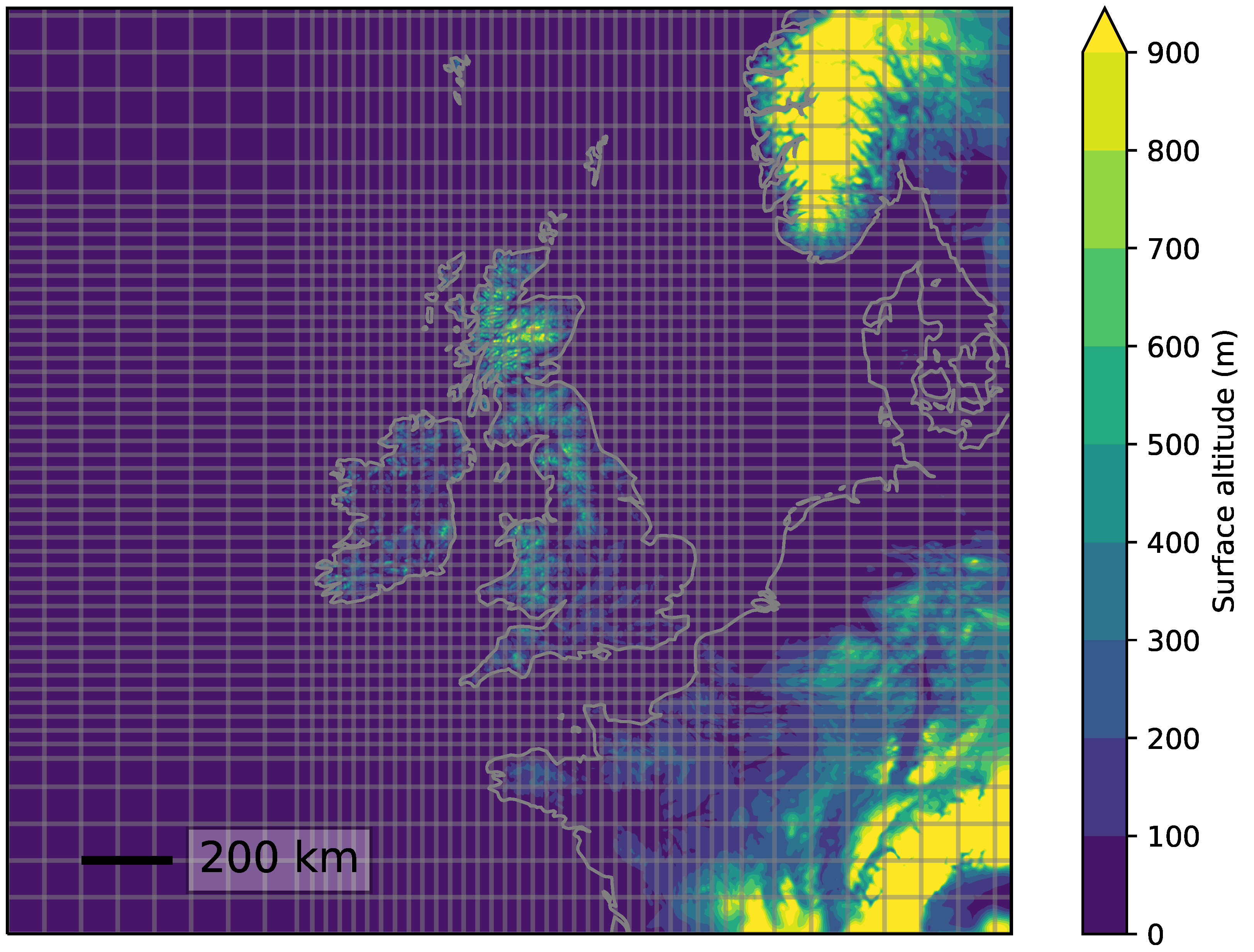
The NWP model used in this study is a high-resolution limited area configuration of the UM, using version 2 of the midlatitude regional atmosphere and land settings (RAL2-M). Version 1 of this configuration has been described previously [
19]. The changes for version 2 relate to the treatment of surface snow, surface exchange, boundary layer physics and cloud microphysics in mixed phase clouds as well as a unification of the vertical level set between the midlatitude and tropical configurations. The model uses a variable-resolution horizontal grid centred over the United Kingdom (
Figure 1), with a grid spacing in the central region of 1.5 km. Note that some of the flights used in this study extend to the outer region of the grid, which has a coarser 4 km resolution. The model has 90 vertical levels on a hybrid-height grid, extending from the surface to a height of 40 km, and is initialised using the analysis from the operational deterministic UKV forecast [
20] closest in time to the flight. The model timestep is 1 min, and atmospheric and surface fields are output every 15 min. For the simulations presented in this study, the fields closest in time to the mid-point of the observations are used. This gives a maximum time difference between observations and model fields of 32 min.
The atmospheric fields required for the radiative transfer simulations consist of pressure, temperature, humidity mixing ratio, surface temperature, surface wind speed (over ocean) and hydrometeor mass contents. The surface wind speed is required to model the sea surface emissivity. Hydrometeors within the RAL2-M configuration are represented using four species: cloud liquid water, rain, graupel and cloud ice. Note that, unlike many models, no distinction is made between non-precipitating and precipitating cloud ice (i.e., ice and snow). A single-moment microphysics scheme is used for each hydrometeor, with the species mass fraction as the prognostic variable. The radiative transfer model requires input atmospheric fields on a constant pressure grid. The NWP fields are therefore interpolated vertically from the hybrid-height grid to a constant pressure grid with 90 vertical levels. The pressure levels are chosen to span the minimum and maximum pressure present in the NWP field, and they approximately match the spacing of the original hybrid-height levels. The maximum spacing between adjacent pressure levels is approximately 20 hPa. To prevent excessive extrapolation from the temperatures available in the hydrometeor scattering database used in the radiative transfer model, any liquid or rain at a temperature less than 230 K is removed as well as any graupel or ice at a temperature greater than 290 K. This results in only minor changes to the hydrometeor mass fields. Small values of hydrometeor mass (less than kg m) are also set to zero to prevent issues within the radiative transfer model.
Radiative transfer simulations were performed using the Atmospheric Radiative Transfer Simulator (ARTS) version 2.3.1277 [
21], and care was taken to ensure that, where possible, the representation of the cloud microphysics is approximately consistent between the NWP and radiative transfer models. This is important as it means that differences between simulated and observed brightness temperatures can potentially be used to diagnose problems with the model microphysics, as well as making it more likely that a single microphysics representation can be applied across the full electromagnetic spectrum. This will be important in the future when all-sky assimilation is extended to cover infrared and solar regions [
22,
23]. The key parameters in the model microphysics scheme are the particle size distribution and the mass–dimension relationship for each hydrometeor species. These govern process rates within the NWP microphysics model, and they are critical in the radiative transfer model for determining bulk scattering properties from particle single scattering properties. However, due to limitations in the available cloud ice scattering properties, it is not possible to ensure a fully-consistent microphysical model, as described below.
Clouds in ARTS are represented as a set of "scattering elements" defined by their number concentration in each grid cell. Here, each scattering element represents a single hydrometeor (i.e., ice crystal or liquid droplet) with a given maximum dimension (
). The size distribution is represented in discretised form by using multiple scattering elements with different values of
to represent each hydrometeor species. The single scattering properties of each element are taken from the state-of-the-art ARTS scattering database [
24]. This provides scattering data calculated using the Discrete Dipole Approximation (DDA) for frequencies between 1 and 886 GHz and temperatures between 190 and 270 K. A range of ice particle sizes are covered (both maximum and volume-equivalent dimensions are provided), and different particle morphologies or "habits" are included, covering single crystals such as hexagonal columns and plates, rosettes, ice aggregates, and rimed particles. Many of the aggregates are generated using a semi-physical aggregation model resulting in particles whose complexity increases with size in a qualitatively realistic manner. Note that all ice particles in the first release of the database are assumed to have random orientation, although later releases include oriented particles. Scattering properties for liquid spheres at temperatures between 230 and 310 K, calculated using Mie–Lorenz theory, are also included in the database. Hydrometeor mass concentrations are converted to scattering element concentrations within ARTS using specified PSD parametrizations and the particle mass and dimension metadata from the scattering database, i.e., the concentration
of scattering element
i is given by
where
is the diameter of particle
i,
is the particle size distribution for the given hydrometeor mass concentration, and
is the size range represented by particle
i, which is given by the trapezoidal integration weight
When the PSD is constructed internally in ARTS, the particle mass–dimension relationship is fitted to a power law given by
and the approximate total mass concentration given by
is set equal to the mass concentration in the NWP field. Since the range of values of
available in the scattering database is finite, and the individual particle masses do not exactly follow a power law mass–dimension relationship, the total mass concentration from the discretised scattering element concentrations (given by
, where
is the mass of particle
i) is generally slightly less than the input mass concentration from the NWP field. The resulting scattering element number concentrations are therefore scaled by the ratio
to ensure consistent mass between the NWP and radiative transfer models.
Different forms of the particle size distribution
are used for each hydrometeor species as well as different particle habits from the scattering database. The rain size distribution is represented using an exponential distribution with parameters from [
25], which is the same size distribution used by the UM. The scattering properties are taken from the "LiquidSphere" habit in the ARTS database. The cloud liquid water size distribution is a gamma distribution using the same parameters as [
13]. Whilst this is not strictly consistent with the UM microphysics scheme, the cloud liquid water particles are small enough to cause negligible scattering at the frequencies used for this study so the impact will be small. The scattering properties are from the "LiquidSphere" habit, but the size range is restricted to particles smaller than 200
μm to reduce the memory required by the radiative transfer simulations; the fraction of mass contained in particles larger than this is negligible.
The graupel size distribution follows the UM, using a gamma distribution with the form
, where
,
,
and
is chosen to give the correct graupel mass concentration according to (
4). Graupel particles in the NWP model are assumed to be spherical with a density of 500 kg m
. The "GemGraupel" habit is used for the scattering properties as it follows this mass–dimension relationship relatively closely, with a maximum difference in particle mass of approximately 25% for sizes greater than 270
μm (at smaller sizes this habit transitions to a hexagonal column with a mass that is only 25% of the assumed mass in the UM).
Cloud ice hydrometeors have the greatest range of particle shapes and are expected to have the largest impact on the sub-millimetre brightness temperatures. The approach used here follows [
13] and uses a single ice crystal shape or “habit” within the radiative transfer simulations. Simulations are performed for different choices of habit to assess the impact of the choice of shape on the modelled brightness temperatures. Although a large variety of ice crystal shapes are observed in real clouds, it is hoped that a single habit will be able to sufficiently represent the average scattering properties to give realistic simulations [
5], and for NWP applications such a pragmatic approach is required in the absence of realistic predictions of particle habits for different clouds types. The size distribution in the UM follows the tropical parametrization from F07, which expresses the PSD in terms of its temperature and second moment
as well as providing an empirical relationship between
and all other moments
as a function of temperature. This permits the second moment
to be determined from the ice water content and particle mass–dimension relationship; (
3) and (
4) are used to determine
as
, permitting
and hence PSD shape to be determined according to the parametrization. The UM assumes the mass–dimension relationship from [
26] given by
where the exponent
is chosen based on theoretical considerations for aggregating particles [
27]. For this choice of exponent,
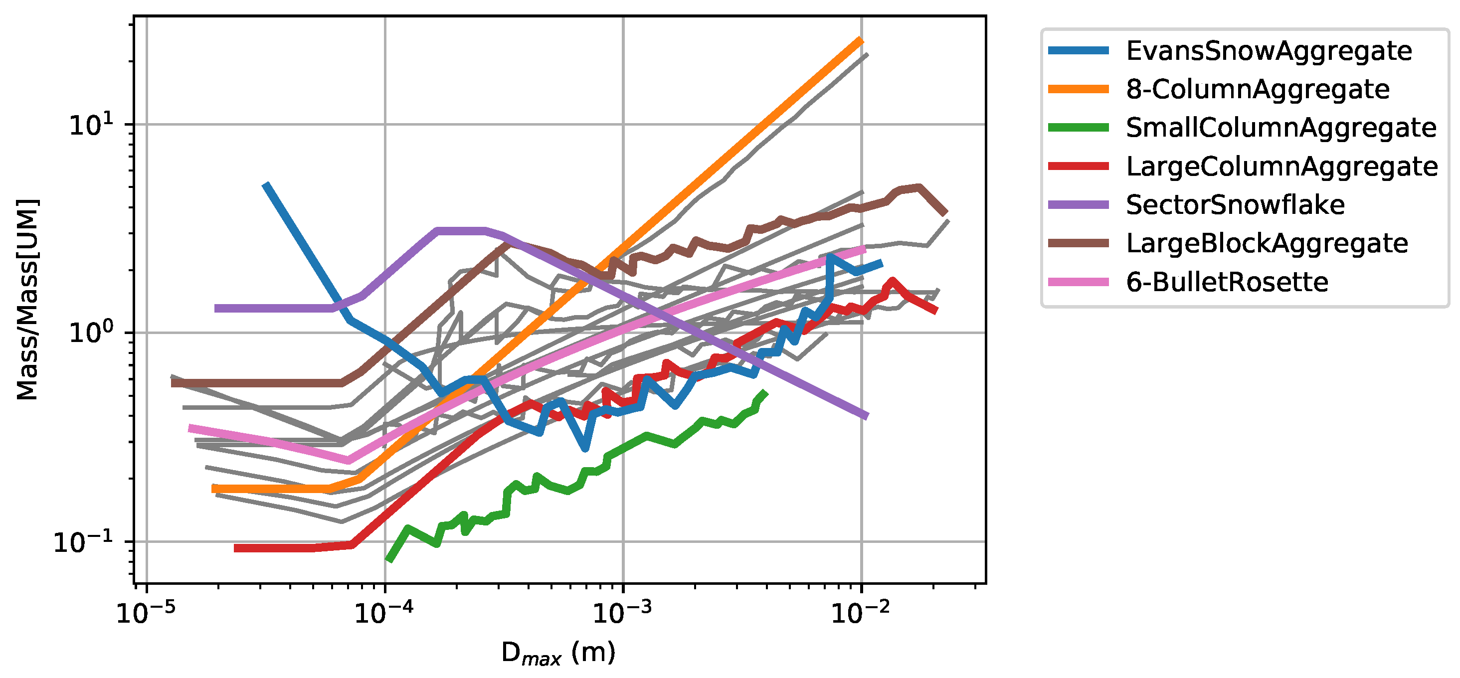
is directly proportional to the ice mass. However, none of the particles in the ARTS database follow this mass–dimension relationship exactly, as shown in
Figure 2, which shows the ratio of the ARTS database particle masses to the mass calculated using (
6) for habits that may be representative of cloud ice. Habits designed to represent hail and graupel are ignored, as are any habits with a mass–dimension relationship exponent of 3, since these are unlikely to be representative of larger aggregated particles. An exception is the “8-ColumnAggregate” shape, originally defined by [
28], which is included as it has been used in previous studies, including for cloud ice retrieval from sub-millimetre observations [
11]. The differences in mass–dimension relationships between the ARTS database and the NWP model mean that it is not possible to match exactly both the size distribution and the ice mass concentration between the NWP and radiative transfer models using single habits from the ARTS database. Instead, the F07 tropical parametrization is used in the radiative transfer model, but the individual mass–dimension relationships of the ARTS database habits are applied. This ensures that the bulk mass remains consistent with the NWP model.
Even with the restrictions on possible cloud ice habits described above, it is still not practical to perform simulations for all remaining habits. A subset of habits was identified according to the bulk optical properties, which have been calculated by integrating the single scattering properties over the F07 tropical PSD for a range of ice water content values.
Figure 3 shows bulk extinction coefficients, single scattering albedos and asymmetry parameters at 175.3 and 670.7 GHz and a temperature of 230 K. A range of particle habits has been selected that covers the range of bulk optical properties, and these particles are indicated by the coloured lines. Note that the SectorSnowflake habit, which was found by [
13] to give good results at frequencies between 10 and 183 GHz, is included in the selected habits. For the selected habits, the mass-weighted mean size (assuming the F07 tropical PSD) ranges between approximately 60% and 200% of that derived using (
6) for ice water contents between
and
kg m
and temperatures between 223 and 263 K.
Simulations in ARTS are performed using the 3D Monte Carlo (3DMC) solver [
29], which permits fully-polarised calculations using the full 3-dimensional model fields and accounts for 3D effects as well as multiple scattering. The first two elements of the Stokes vector are calculated, although polarisation effects due to clouds in the simulations will be small, as all particles in the first release of the ARTS scattering database are assumed to have random orientation. Polarisation effects due to clouds are therefore not considered in the present study, and the main source of polarisation differences will be surface reflections, particularly for the lowest frequency window channel at 89 GHz. The target estimated error for the Monte Carlo solver is set to 0.5 K with a maximum iteration time of 1200 s for each simulated frequency and observation. The majority of the simulations converge to the required accuracy within this time; the exception is frequencies with significant surface sensitivity over the ocean where estimated errors of order 1 K can occur. Note that although the 3DMC solver permits highly-accurate calculations, it is too slow for many operational applications, and fast scattering radiative transfer models will be required for practical implementations of all-sky assimilation.
Following the approach used by previous studies [
11,
12], for dual-sideband channels which simultaneously measure on both sides of a gaseous absorption line, the simulations are performed for monochromatic frequencies at the centre of each of the two sidebands and averaged. For window channels a single monochromatic frequency at the nominal channel centre is used. This approach means that gaseous absorption due to ozone is neglected, since the relevant ozone lines are significantly narrower than the channel bandwidths. However, since the aircraft is generally below the tropopause, the impact of ozone on measured downward-looking brightness temperatures is expected to be small. For satellite observations the effect of ozone can be up to 1.6 K at 664 GHz [
1]. Water vapour resonant absorption is calculated using line parameters from the AER database v3.6 [
30], which is based on HITRAN-2012 [
31] but includes modifications to key atmospheric absorption lines based on a number of sources. A Voigt line shape with a Van Vleck–Huber pre-factor and a cut-off at 750 GHz from the line centre is used, and the water vapour continuum absorption is calculated using MT–CKD v3.2 [
32]. These water vapour absorption properties include updates in the sub-millimetre and microwave regions as a result of observations taken during the Radiative Heating in Underexplored Bands Phase II (RHUBC-II) campaign [
33]. Oxygen absorption parameters are taken from [
34], and the nitrogen continuum absorption follows [
35].
The simulations are performed using a Gaussian antenna pattern with the same full-width half-maximum beamwidth as the observations. The mean aircraft position, altitude and sensor line-of-sight over the 1.5 km observation averaging distance is used. The surface emissivity over the sea is estimated using the TESSEM2 model [
36], and land is treated as a specular surface with a reflectivity of 0.1.
4. Results
This section compares the simulated brightness temperatures with observations from MARSS and ISMAR for the five case studies described above. Firstly, the difference between simulated and observed brightness temperatures at each location along the flight tracks is considered. This is indicative of the first-guess departures that might be seen within an all-sky assimilation system, and it will include differences due to mis-location of cloud features within the NWP model as well as errors in the cloud microphysics and radiative transfer calculations. Statistical properties that are less sensitive to errors in cloud position, such as brightness temperature histograms, are then considered in order to assess the adequacy of the cloud microphysics representation within the models. Note that for downward-looking views at the frequencies considered here the brightness temperature is linearly related to the radiance, but has the advantage that it is scaled such that direct comparisons can be made between observations at different frequencies.
Figure 6 compares the observed and simulated brightness temperatures along the aircraft track for each case study flight for the 89, 243 and 664 GHz channels. These have been chosen to illustrate the behaviour across the range of frequencies available, and since they are quasi-window channels they show the greatest sensitivity to the presence of cloud at all altitudes. Equivalent plots for the other available channels can be found in the
supplement (Figures S5–S9). To emphasize the signal due to cloud, the plots show the difference between the observed or simulated brightness temperatures and equivalent "clear-sky" simulations. The clear-sky simulations account for gaseous absorption and emission, and surface emission and reflectance, but they do not include scattering or absorption from cloud hydrometeors. For the simulations, the difference between cloudy and clear-sky brightness temperatures is a true representation of the signal from the cloud, but for the observations it also includes differences due to any errors in model temperature and water vapour fields, surface properties and gas spectroscopy. For example, during B984, C159 and C161 brightness temperature differences between observations and clear-sky simulations are seen for all channels close to the centres of the water vapour absorption lines at 183, 325 and 448 GHz (
Figures S6, S8 and S9). This suggests there are errors in the NWP model upper tropospheric water vapour. Nevertheless, the differences are generally small for scenes containing little cloud, which gives confidence that the clear-sky simulations are sufficiently accurate to derive the cloud signal from the observations for all but the thinnest clouds. For channels where only a single polarisation is observed, the horizontal and vertically-polarised simulations have been appropriately combined to give the brightness temperature at the observed polarisation. For channels where dual polarisation is observed, the simulated intensity is plotted and the observations are shown for both polarisations. Note that since all ice crystals are assumed to have random orientation, the simulated polarisation difference will be small for channels which are not generally sensitive to the surface, i.e., all channels except 89 and 157 GHz. The primary surface type for each observation (land or sea) is indicated by the background shading on the 89 GHz plots.
Brightness temperature signals due to clouds are clearly seen in all channels. At 89 GHz the effect is primarily an increase in brightness temperature above the clear-sky value for points over the sea, due to the effect of liquid water absorption and emission, and the low surface emissivity. Signals are generally much smaller over land (e.g. during parts of B984 and most of C161), due to the high surface emissivity, which means that the upwelling brightness temperature at the surface is close to the emitting temperature of the liquid clouds. Snow and ice covered surfaces were not observed during these flights, but they would be expected to have highly variable emissivity caused by changes in snow microstructure and stratigraphy [
37], which makes simulations of surface-affected observations challenging. Since scattering from cloud ice is weak at this frequency, there is little difference between the simulations for different ice particle habits. An exception is the 8-ColumnAggregate, which gives brightness temperature depressions for the highest ice water paths during B984, C159 and C161. However, these scattering signals are not seen in the observations, suggesting that this habit has unrealistically large scattering at this frequency. It is interesting to note that over the sea, the observed brightness temperatures at 89 GHz are generally smaller than the simulated brightness temperatures, and they are closer to the clear-sky values. This suggests that the NWP model is over-predicting the amount of cloud liquid water and rain for these cases.
Frequencies higher than 89 GHz show significantly more sensitivity to scattering from cloud ice, with large brightness temperature depressions relative to the clear-sky values. At 157 GHz there are both increases due to liquid water absorption and decreases due to ice scattering, whereas from 183 GHz and beyond there is little sensitivity to cloud liquid. This is due to a combination of increased sea surface emissivity and masking of emission from the lowest atmospheric layers due to water vapour absorption, even in nominal window channels. For four of the flights (B984, C156, C159 and C161) there is good agreement in the overall characteristics of the cloud features, including their location, between the simulations and the observations although some details differ. For B949, the simulations do not predict the large decrease in brightness temperature observed at 157 and 243 GHz up to approximately 200 km along the aircraft track. This corresponds to the region of rainfall on the image in
Figure 4, so the discrepancy is likely to be caused by a misrepresentation of the cloud field within the NWP model. It can also be seen in
Figure 6 that the different channels are sensitive to different cloud altitudes. For example, during the central part of C159 there are large brightness temperature depressions at 243 GHz whereas the cloud signals at 664 GHz are smaller than for the other flights. This is a consequence of the relatively low cloud-top altitude (between 7 and 8 km) for this flight, since the 664 GHz channel is mainly sensitive to ice in the upper troposphere due to water vapour absorption at lower altitudes. In contrast, larger brightness temperatures depressions are seen during C161 between 200 and 300 km along-track at 664 (and 874) GHz compared to 243 GHz. This corresponds to the cirrus cloud predicted by the model between 7 and 10 km altitude (
Figure 5), which consists mainly of smaller ice crystals and causes less scattering at the lower frequencies.
As might be expected from the wide range of bulk optical properties (
Figure 3), there are considerable differences between the simulations using different particle habits. This is particularly noticeable at 243 GHz, where brightness temperature depressions vary by more than 70 K between the different particle habits at some times during the flights. The maximum difference between the simulations for the different habits at 664 GHz is smaller (approximately 40 K), but it is still significant. The observations mostly lie within the range of the simulations for the different habits, and they are generally closer to the middle of the range of simulated values than either of the extremes. An exception to this is the large spikes seen in the 243 GHz observations during the first part of C161 and between 150 and 200 km along track during C159. These are thought to correspond to the presence of large ice particles in shallow convective clouds (e.g. behind the cold front during C161) which are not represented by the NWP model. For C161, between 300 and 400 km the simulated brightness temperatures are generally significantly lower than the observations at 664 GHz. This is probably due to differences in timing and location of the highest IWP values between the model and reality, since the largest brightness temperature depressions are of similar magnitude in the simulations and observations, albeit with the large depression in the observations occurring over a shorter extent. Note that this offset in location is consistent with the relatively rapid south-eastward progression of the cold front during this flight. For C156 the observed brightness temperature depressions at 664 GHz are closer to the simulations for the more extreme habits, and at 874 GHz (
Figure S7) they lie significantly outside the range of simulated values. Analysis of in-situ measurements of bulk ice mass for this case, made immediately after the above-cloud runs, suggests that the NWP model may be significantly underestimating the mass of ice between 2 and 7 km during this flight. This would result in the simulated brightness temperatures depressions being too small at these frequencies.
Figure 7 shows the statistics (bias and RMSE) of the first-guess departures, i.e., the difference between observed and simulated brightness temperatures, using different ice particle habits. For clarity, only window channels and these furthest from the centre of gas absorption lines are shown as they will be most sensitive to cloud scattering. Results for all channels can be found in
Figure S10 in the supplement. Many channels, particularly at frequencies above 157 GHz and away from the centre of gas absorption lines, show strong sensitivity to the ice particle habit. The greatest sensitivity to particle habit for these cases occurs at 243 GHz. Note that for the flights studied here, high ice masses generally only occur at lower altitudes, where the higher frequencies are less sensitive due to water vapour absorption. If large ice masses were to occur at high altitudes the higher frequencies could also become more sensitive to the particle habit. For example, [
38] showed a stronger sensitivity to particle habit at 668 GHz compared to 190 GHz over the tropical Pacific. At all frequencies other than 89 and 874 GHz it is possible to find a particle habit that has a bias close to zero, and particles with small biases generally also have lower values of RMSE at a given frequency. The large bias and RMSE at 89 GHz is due to the liquid water as discussed above, and this will also impact the 157 GHz results. At 874 GHz the statistics are strongly influenced by flights C156 and C159 as the channel was only available on three of the five flights. As discussed above, it is likely that for C156 the NWP model has too little ice at higher altitudes. During C159, the the 664 GHz observations are generally close to the simulated clear-sky values whereas the 874 GHz observations are colder than the clear-sky values (
Figure S8). This suggests that there may be an uncorrected bias of around 5 K in the 874 GHz observations for this flight.
The EvansSnowAggregate and SmallColumnAggregate habits generally have insufficient scattering, leading to negative biases, whereas the 8-ColumnAggregate, SectorSnowflake and LargeBlockAggregate are over-scattering. The 6-BulletRosette and LargeColumnAggregate show good performance across all the frequencies, with the LargeColumnAggregate having slightly smaller RMSE. Between 183 and 664 GHz the LargeColumnAggregate bias is less than 3 K and the RMSE is less than 10 K, with the exception of the horizontally-polarised 243 GHz channel where they are −5.6 K and 12.5 K respectively. The difference between the statistics for the horizontally and vertically-polarised channels at this frequency suggests that there may be some horizontal orientation of ice particles which cannot be simulated using the randomly-oriented particles available in the ARTS scattering database. These errors can be compared to the observation errors used in the all-sky assimilation system being developed at the Met Office [
39]. For the 190.3 GHz channel on the Microwave Humidity Sounder (MHS) the error model assigns an observation error of 1.7 K in clear sky conditions. The error varies linearly with ice water path and liquid water path; using the average across all flights of the mean values of ice and liquid water path from
Table 2 gives a modelled observation error of 2.6 K. The RMSE at 183 ± 7 GHz for the LargeColumnAggregate is larger than this (3.9 K), but it should be noted that the MHS observations in the Met Office system are averaged over a footprint of approximately 40 km, compared to the 1.5 km used for the airborne observations. This makes a direct comparison difficult, and it is expected that the RMSE will decrease with increasing footprint size. It is encouraging for future all-sky assimilation of ICI that many of the higher-frequency channels can be simulated with similar accuracy to the 183 ± 7 GHz channel.
It is interesting to note that the LargeColumnAggregate was found by [
38] to give a good match to observations from the GPM Microwave Imager between 166 and 190 GHz. However, it should be noted that this conclusion was mainly based on simulations using the PSD from [
40], which predicts a much larger proportion of small ice particles than the F07 tropical PSD used here. Nevertheless, they found broadly similar results using the F07 tropical PSD because their method of determining the IWC from CloudSat radar reflectivities and particle backscattering properties is relatively insensitive to the assumed PSD, in contrast to simulations using fixed IWC fields which show strong sensitivity. The 8-ColumnAggregate, which was used by [
11] for ice water path retrievals, performs very poorly. It has a large bias and RMSE, particularly at the lower frequencies, where it has too much scattering. The SectorSnowflake, which was preferred as a single globally-representative habit by [
13] for frequencies up to 183 GHz, performs relatively poorly at higher frequencies, where it predicts too much scattering. However, that study showed similar excess scattering at 183 GHz in the mid-latitudes but found the stronger scattering was required to give a good match to the satellite observations in the tropics. This may be a result of compensating errors; it was shown by [
41] that the ERA5 reanalysis underestimates the IWC when compared to DARDAR [
42] retrievals in the tropical upper troposphere, so a strongly scattering particle may be required to compensate for insufficient ice mass in the NWP model.
Statistics such as RMSE are affected by the well-known “double-penalty” effect, where an error in cloud position in the NWP model leads to larger RMSE than simply having no cloud in the model at all. Previous studies have compared brightness temperature histograms as they are robust to this effect, as well as allowing comparisons where, for example, co-location between observations and simulations is not available [
13,
38]. Although the sample size available in this study is rather small, it is still interesting to consider the brightness temperature histograms, which are shown for selected channels from all flights in
Figure 8. The histogram fit statistical metric proposed by [
13], given by
i.e., the mean logarithm of the ratio of the populations in each histogram bin, is also plotted in
Figure 9. This metric is designed to give equal weight to each histogram bin, regardless of the number of occurrences in each bin, with lower values indicating a better match between the histograms. The brightness temperature histograms do not show the strong clear-sky peak seen in other studies because the airborne observations specifically target cloudy scenes. There are no clear discrepancies between the observed and simulated histograms, except at 874 GHz where the observations show a greater number of occurrences of relatively low brightness temperatures between approximately 185 and 200 K. However, as noted previously, the statistics for this channel are strongly influenced by two cases which may contain observations with a significant cold bias. There are also differences between the horizontally and vertically-polarised observations at 243 and, to a lesser extent, 664 GHz, particularly at the coldest brightness temperatures. These are consistent with the presence of horizontally-oriented particles. The most prominent differences between the simulations for different particle habits relate the frequency of occurrence of low brightness temperatures, particularly in channels that are not close to the centres of gas absorption lines. Consistent with the results above, the strongest sensitivity to particle habit occurs at 243 GHz, and at frequencies above 448 GHz the differences in the histograms are relatively small. The histogram fit parameter shows the same trends as the RMSE. Of the particle habits used in this study, the LargeColumnAggregate has the best performance on average across the range of frequencies.
5. Discussion and Conclusions
The results presented in the previous section demonstrate that it is possible to simulate realistic sub-millimetre brightness temperatures for cloudy scenes using atmospheric fields from a state-of-the art high-resolution NWP model and an accurate radiative transfer model with a realistic representation of cloud ice scattering. This is a necessary first step towards using sub-millimetre observations within an all-sky assimilation system. However, the fit between the observed and simulated brightness temperatures is strongly dependent on the selected cloud ice particle shape, even though the total ice mass and (as far as possible) the shape of the particle size distribution, are kept constant. For the cases studied here, the sensitivity to the assumed particle habit is strongest at 243 GHz, but stronger sensitivity at higher frequencies is expected if there is greater ice mass at higher altitudes.
For the flights used in this study, a single particle habit with random orientation, the LargeColumnAggregate, is able to reproduce observed brightness temperatures between 183 and 664 GHz (i.e., the frequency range covered by ICI) with a bias of less than 3 K and RMSE less than 10 K for all channels other than the horizontally-polarised 243 GHz channel. Of course this result, which is based on a limited number of observations of midlatitude frontal cloud, may not be globally applicable in all cloud regimes. Nevertheless, it is interesting to note that the same particle habit was shown by [
38] to simulate brightness temperatures consistent with GPM Microwave Imager observations between 166 and 190 GHz when using cloud fields based on CloudSat radar reflectivities over the tropical Pacific, although their best fit used a different PSD. Once sub-millimetre observations from ICI become available, it will be possible to follow the methodology of [
13] and use global statistics of first-guess departures to test the applicability of a single representative particle habit and select the optimum ice crystal shape for use in an all-sky assimilation. Furthermore, as all-sky assimilation systems evolve in the future to use a greater range of the electromagnetic spectrum, including infrared and solar regions [
22,
23], it will be desirable to have a physically realistic representation of cloud ice microphysics and optical properties that is consistent across all wavelengths [
43]. This may also permit the same physical representation of cloud ice to be used in both the data assimilation and NWP model cloud microphysics and radiative flux schemes, and would allow more robust comparisons between models and satellite observations.
The results at 89 GHz suggest that the NWP model is over-predicting the occurrence of cloud liquid water for these cases. However, this is dependent on the cloud regime. For example, previous studies show that there is insufficient cloud liquid water in the UM during cold-air outbreak conditions [
44]. The high sensitivity of the simulated brightness temperatures at higher frequencies to the assumed particle habit means that it is not possible to use the observed sub-millimetre brightness temperatures alone to place strong constraints on the NWP model ice cloud microphysics scheme. For example, an under-prediction of ice water content in the NWP model could be compensated for by using a particle habit with stronger scattering to give similar brightness temperatures. Likewise, errors in the assumed particle size distribution used in the NWP and radiative transfer models could be compensated by using an ice particle habit with different scattering properties. Whilst these compensating errors may provide a pragmatic solution to permit the implementation of an all-sky assimilation system, it is preferable to identify and rectify any underlying model deficiencies. Using observations covering a greater portion of the electromagnetic spectrum that have sensitivity to different regions of the particle size distribution, including visible and infrared observations, as well as considering active measurements such as multi-frequency radar and lidar, could place stronger constraints on the representation of cloud within the models. However, the availability of suitable datasets is currently very limited, although it should be noted that during FAAM flight B984 the German HALO and French Safire Falcon aircraft made simultaneous observations with 35 and 94 GHz cloud radars, lidar, passive microwave and visible instruments. In addition, the flight tracks during C159 and C161 followed overpasses of CloudSat and CALIPSO. Further analysis of these combined active and passive datasets is ongoing. There is also currently a lack of ice particle scattering data that makes consistent assumptions at all wavelengths, and the ice crystal models used to generate scattering databases do not always follow the same mass–dimension relationships assumed by the NWP models. Development of fully-consistent ice crystal models is also an area of ongoing research.
The ARTS 3DMC solver used in this study permits accurate calculations of fully-polarised brightness temperatures, but it is too slow to use within an operational assimilation system. Practical application of all-sky assimilation to ICI observations will require fast radiative transfer models such as RTTOV-SCATT [
45] to be extended to cover sub-millimetre frequencies with sufficient accuracy. Consideration may also need to be given to the impact of the sub-cloud heterogeneity within the relatively large (16 km) ICI footprint as well as the coarser resolution typical of global NWP models. However, the success of all-sky assimilation at frequencies up to 183 GHz in current global NWP systems suggests that these issues need not prevent ICI observations from having a positive impact on NWP forecasts by providing additional information on the location and microphysical properties of ice clouds.


