Comparison of Harmonic Analysis of Time Series (HANTS) and Multi-Singular Spectrum Analysis (M-SSA) in Reconstruction of Long-Gap Missing Data in NDVI Time Series

Abstract

Monitoring vegetation changes over time is very important in dry areas such as Iran, given its pronounced drought-prone agricultural system. Vegetation indices derived from remotely sensed satellite imageries are successfully used to monitor vegetation changes at various scales. Atmospheric dust as well as airborne particles, particularly gases and clouds, significantly affect the reflection of energy from the surface, especially in visible, short and infrared wavelengths. This results in imageries with missing data (gaps) and outliers while vegetation change analysis requires integrated and complete time series data. This study investigated the performance of HANTS (Harmonic ANalysis of Time Series) algorithm and (M)-SSA ((Multi-channel) Singular Spectrum Analysis) algorithm in reconstruction of wide-gap of missing data. The time series of Normalized Difference Vegetation Index (NDVI) retrieved from Landsat TM in combination with 250m MODIS NDVI time image products are used to simulate and find periodic components of the NDVI time series from 1986 to 2000 and from 2000 to 2015, respectively. This paper presents the evaluation of the performance of gap filling capability of HANTS and M-SSA by filling artificially created gaps in data using Landsat and MODIS data. The results showed that the RMSEs (Root Mean Square Errors) between the original and reconstructed data in HANTS and M-SSA algorithms were 0.027 and 0.023 NDVI value, respectively. Further, RMSEs among 15 NDVI images extracted from the time series artificially and reconstructed by HANTS and M-SSA algorithms were 0.030 and 0.025 NDVI value, respectively. RMSEs of the original and reconstructed data in HANTS and M-SSA algorithms were 0.10 and 0.04 for time series 6, respectively. The findings of this study present a favorable option for solving the missing data challenge in NDVI time series.

1. Introduction

Monitoring vegetation coverages over time is highly important and is applicable to many research fields, including management of natural, water and agricultural resources [1,2,3,4]. Nowadays, rapid and wide-area monitoring of changes in natural resources including vegetation is possible due to the development of remote sensing technologies and access to satellite images of the past decades. Many of the studies of vegetation such as long-term interactions between plants and climatic changes require integrated, gap-free and complete temporal data. However, the integrity of remote sensing data can be dramatically altered due to influences of atmospheric dust, aerosols, clouds as well as measurement sensor failure and algorithm malfunctioning, among others [5]. In this regard, clouds are one of the most important factors involved in causing missing data (gaps), outliers and noise in satellite images [6]. Missing data (gaps) imply absence of valid surface observations due to cloud coverage or failure of retrieval. On the other hand, outliers are characterized as unusual values that deviate from the normal variability in the dataset [7,8]. Clouds are often indicated in satellite images by characteristic higher reflection and lower surface temperature than other terrestrial phenomena in visible and thermal electromagnetic spectral ranges, respectively [9,10].

Vegetation changes can be studied by remote sensing using indices which are usually calculated using red and near-infrared spectral data as inputs [11]. Since most vegetation indices are calculated using red and near-infrared bands, the presence of clouds brings about missing and remote data or outliers. The amount of cloud cover-induced missing data depends on the degree of cloudiness of different regions during the year and in various seasons. Based on experiments done by Ghanaian (2015) and Jia et al. (2011) to evaluate the effect of gap size (defined as a period with continuously missing data) in reconstruction of the Land Surface Temperature (LST) and NDVI time series, the threshold gap size is correlated to the longest period in the time series. The gap size in a time series can be classified into short or long gaps. A short (long) gap is shorter (longer) than the period of time sampled by half of the observation points [12]. Different algorithms have been developed for noise reduction and filling of missing data in time series [13]. Harmonic ANalysis of Time Series (HANTS) algorithm was introduced by Verhoef in 1996 for reconstruction of outliers and missing data simultaneously in time series with periodic behavior. This algorithm has two objectives [14] which are (i) identification and removal of remote points and cloud observations and (ii) filling the remaining gap among observations by temporal interpolation.

A variety of methods have been used for filling gaps in multi-temporal spatial data. Johnson (2002) used asymmetric Gaussian functions which extracts phenological parameters and reconstruct smooth time series. The method, however, could not effectively discriminate between maxima and minima that come from seasonal variation and those from noise. The method was also unsuccessful where noise level was high or the growing season was short thus requiring input from other algorithms such as Fourier series [15]. Beck et al. (2006) developed a method based on double logistic function which describe NDVI data better than the Fourier and slightly better than the asymmetric Gaussian without overestimating the duration of the growing season [16]. Chen et al. (2004) developed another method based on the Savitzky–Golay filter to smooth out effect of cloud contamination and atmospheric variability on NDVI time series. The method was effective in obtaining high-quality NDVI time series [17]. Cao (2018) further developed the Spatial Temporal Savitzky Golay (STSG) method which performed better than the Asymmetric Gaussian, Double Logistic, Fourier based and Savitzky Golay filter methods [18]. Assessment of Fourier analysis, asymmetric Gaussian model, double logistic and the Whitaker filter by Atkinson (2012) showed that comparative performances of the methods vary with context. For example, although the Double Logistic outperformed others when simulated data were used, it performed less well on real data. For data extracted from remotely sensed images, the Whitaker approach outperformed others but underperformed when applied to noisy data. Therefore, comparative studies must identify the context under which a model perform better than others [19].

HANTS algorithm is also used to reconstruct the missing and remote NDVI time series data [14,20,21,22]. Zhou et al. (2015) evaluated the performance of HANTS algorithm in reconstructing global MODIS NDVI time series [23]. Jiang et al. (2008) reconstructed the effect of cloud cover on AVHRR NVDI time series during 1981–2001 using HANTS algorithm [24]. In another study, Zare Khormizi et al. (2017) studied the capability of HANTS algorithm in reconstruction of one- and five-year MODIS NDVI time series [2]. The results of these studies showed that HANTS algorithm can be used to effectively resolve the problem of missing data in NDVI time series analysis. The advantages of HANTS algorithm are its simplicity, low computational cost and accuracy, especially when the gap size is short and it is not at the beginning or end of the time series. However, its disadvantage is that it only uses temporal correlation (compared to the methods using spatial-temporal correlation) to fill the gaps in time series. Therefore, when HANTS is applied in a temporal series with long contiguous gaps, the Fourier coefficients are less accurate because they are calculated using less temporal information. For this reason, the reconstruction of the temporal series is less precise than using a temporal series with shorter gaps.

Broomhead and King [25,26] and Broomhead et al. [27] proposed Singular Spectrum Analysis (SSA) as an advanced technique for time series analysis. Since then, the technique has attracted a lot of attention by researchers involved in technical aspects and applications [28,29,30,31,32]. SSA decomposes a time series into simpler, interpretable components such as a trend, various oscillatory components (periodic and quasi-periodic) and noise as the main purpose. The underlying concept in SSA properties is “separability” which describes the extent to which different components can be discriminated from each other [33]. Regular (cycles) and irregular (noise) components are often included in the temporal evolution of the observations. SSA uses Empirical Orthogonal Function (EOF) analysis to extract information from noisy and short time series without apriori knowledge of the dynamic processes influencing the underlying time series [31]. The main objective of this multivariate analysis technique is to transform a set of time-dependent (often) variables into a smaller set of variables that are uncorrelated. The first components of this multivariate analysis project the dependent variables onto the directions of largest variance [34]. The first components are those that capture most variance in the data, while the other components may be considered as noise.

In meteorological and geophysical time series data analysis, SSA has already become a standard and very successful tool [32,35,36,37,38,39,40]. In a study by Ghafarian et al. (2012), an hourly-LST time series was reconstructed using Multi-Singular Spectrum Analysis (M-SSA), i.e., an extension of SSA algorithms. The results showed a Mean Absolute Error (MAE) of 2.25 K between the original and reconstructed time series with an average of 63% of missing data caused by cloud cover [5]. In [41], the authors reconstructed the missing data in the Leaf Area Index (LAI) of the MODIS sensor using the M-SSA algorithm. They showed that spatio-temporal correlation capability of M-SSA reconstructs this index effectively. However, despite its potential, the M-SSA has rarely been used to reconstruct NDVI time series. Furthermore, while the individual performances of HANTS and M-SSA are well documented, comparative studies of the gap filling capabilities of the two methods are generally lacking especially about improving NDVI data availability for land surface characterization. As a result, there is a paucity of literature describing the scenarios under which the methods alternately outperform each other.

The present study thus aimed to evaluate and compare the performance of HANTS and (M)-SSA algorithms in reconstruction of long-gap missing data in Landsat 5 TM NDVI time series. In order to achieve this, firstly, the main periodic components of NDVI time series are extracted. As the original Landsat data has gaps and outlier, a 250-m MODIS NDVI time series product (without gaps and outliers), with the same period length of LANDSAT TM image, was utilized to find periodic components representing the dynamic of NDVI time series and also validation of the results. These parameters are then used to reconstruct the Landsat NDVI time series. The gap-filling capability of HANTS and SSA were examined by creating artificial gaps in the original MODIS NDVI time series and compared the results with them. The reconstruction capability of HANTS and SSA has been examined by comparing the original and reconstructed data at valid data points.

2. Materials and Methods

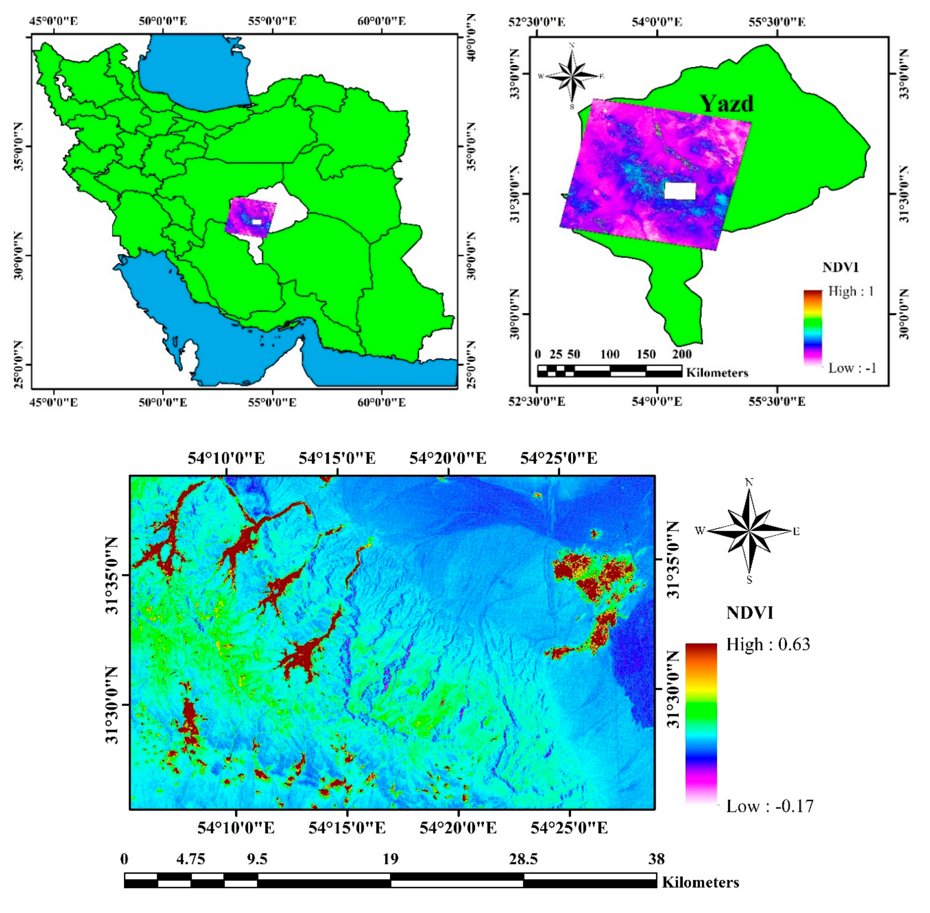
2.1. Study Area

The study region in the present research is located between latitudes 31°26′ and 31°39′N and longitudes 54°5′ and 54°29′E from prime meridian. This region is situated in Yazd province, Iran (Figure 1). The lowest elevation of the area is 1400 m and the highest elevation is 3800 m from the sea level. Average precipitation for the whole study area is 150 mm, while the amount comes to 60 mm in low elevation places and 230 mm in higher places [42,43,44,45,46,47].

The highest percentage of vegetation coverages are clustered in the regions where villages and gardens are located (brown color regions). In contrast, natural vegetation and pastures cover less than 30% of the area since the region has a dry climate. The dominant vegetative form of the study area are the shrubs such as Artemisia sieberi, Artemisia aucheri, Austragalus sp., Amygdalus scoparia.

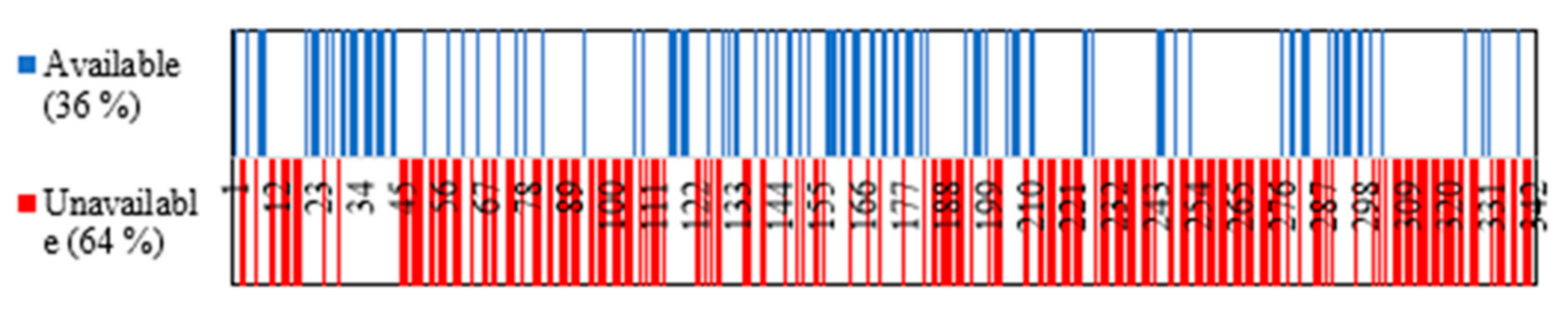
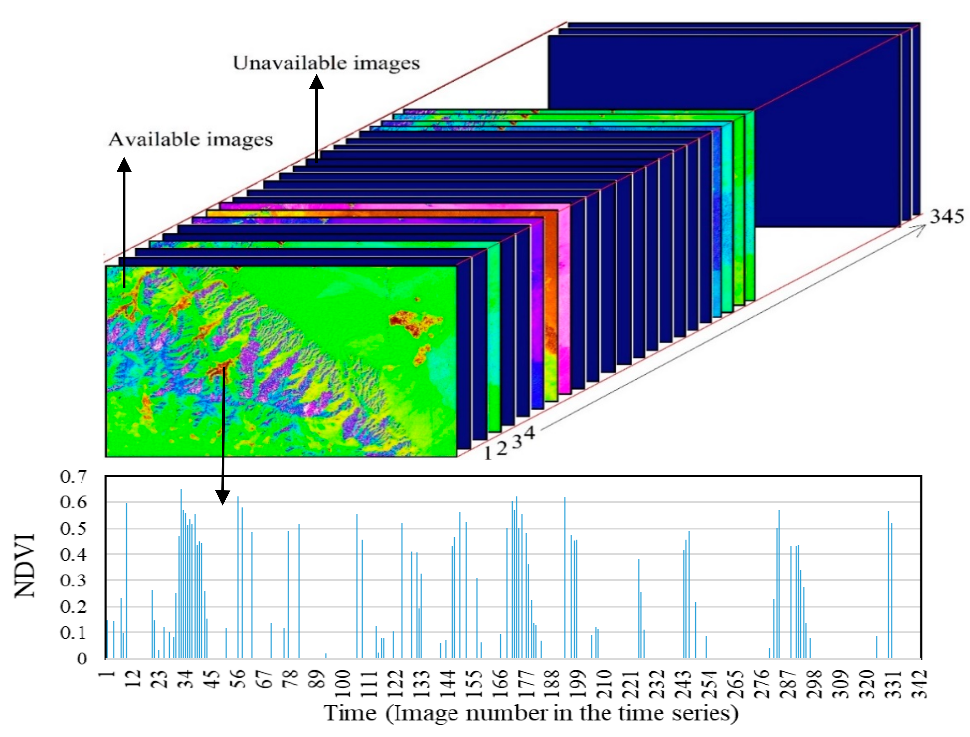
2.2. Satellite Images Time Series

Landsat 5 TM images were used in this study. Landsat 5 TM sensor has 7 spectral bands, within which the thermal infrared band 6 has a spatial resolution of 120 m while other bands have a resolution of 30 m [48]. Totally 122 available images spanning from 1986 to 2000 were obtained from the United States Geological Survey’s website (https://earthexplorer.usgs.gov). The images were used for the analysis and comparison of HANTS and M-SSA algorithms for reconstruction of unavailable data, assuming that the unavailable data were lost due to cloud contamination. Since the extraction of the M-SSA parameters requires gap-free and continues data, MODIS 16-day NDVI products with no gaps and spatial resolution of 250 m in the study region were used. They were also employed to validate the reconstruction results by creating artificial gaps. The extracted periodic components of NDVI changes along a pixel during 2000–2015 were used by M-SSA to reconstruct the Landsat NDVI time series. Like the NDVI time series of LandsatTM sensor, we had a similar 15-year time series of MODIS NDVI products with 345 images. The Landsat NDVI was calculated as follows [49]:

$$\mathrm{NDVI}=\frac{NIR-RED}{NIR+RED}$$

(1)

where NIR is the spectral reflectance of near-infrared band (at 0.76–0.90 µm) and RED is the red band of TM sensor (at 0.63–0.69 µm).

Considering the revisiting time of Landsat 5 TM sensor, a total of 345 (~23 images per year × 15 years) NDVI images should be available from 1986 to 2000. Figure 2 illustrates the distribution and dispersion of unavailable and available images in the 15-year time series of NDVI. More than 64% of the data of this time series were temporarily unavailable. Figure 3 shows the arrangement of a part of this time series with 345 NDVI images during 1986–2000 along with NDVI changes on a pixel.

2.3. HANTS Algorithm

HANTS algorithm, also known as Fourier analysis, was developed to decompose periodic time dependent data into sum of sinusoids. Therefore, HANTS limits the outliers and fills the missing or cloudy observations in time series data with periodic behavior [14] as well as models satellite data time series based on discrete Fourier transform [11,12,14,20,22,35,50]. A Fourier series can describe a sequence of N temporal acquisition (y_i, i = 1 to N) as:

$$y_i=a_0+{\displaystyle \sum _{j=1}^M{a}_j\cos \left({\omega }_j{t}_i-{\phi }_j\right)}$$

(2)

where the frequency of jth harmonic term is ω_j, t_i is the time at which the ith sample was taken, M is the number of frequencies of the Fourier series (M <= N), φ_j and a_j are the phase and amplitude of the jth harmonic term, respectively. The amplitude related to the zero frequency, a₀, is equal to the average of all N observations of y because the zero frequency has no phase. The harmonic frequencies are a base frequency (i.e., ω₁ = 2π/N) and all integers (i.e., i = 1 to N) are multiples of the base frequency:

$${\omega }_i=(2\pi /N)\times i{,}_{} {}_{}where{ }_{ }i=1,2,...{,}_{}N$$

(3)

After selecting the frequencies (ω_j) and the number of frequencies (M), the phase φ_j and amplitudes a_j are the unknown parameters of the Fourier series in the HANTS algorithm, determined by fitting the time series of observations.

Ref. [8] describes parameters which must be defined by users in order to assign in HANTS to get a reliable signal. These parameters are valid data range (acceptable range of observations), period, Number Of Frequencies (NOF), direction of outliers (direction of outliers with reference to current time series), Fit Error Tolerance (FET, specifies the absolute maximum deviation from fitted curve) and Degree Of Determinedness (DOD, minimum number of extra data points which will be needed for curve fitting). Preliminary tests can help to get some idea about the parameters such as NOF (determined, for instance, from an earlier Fast Fourier Transform (FFT) analysis) since there is no direct way to determine them. The detailed information about the HANTS parameter estimation can be found in [8].

2.4. Singular Spectrum Analysis Algorithm

The gap-filling using SSA and smoothing algorithm follows a procedure based on [5,51]. SSA is based on Singular Value Decomposition (SVD), which is a well-known factorization matrix process. The SVD has been used in remote sensing for different applications such as feature extraction [52] or spatio-temporal analysis [53]. In the latter application, the SVD is also known as Empirical Orthogonal Functions (EOFs) in climatology science. The SVD factorizes the matrix ($X\in R^{m\times k}$) in singular values and vectors as: X = D × ∑ E^T, where D∈ R ^m×m is made up by right singular vectors, E ∈ R ^K×K is made up by the left singular vectors and $\sum$ is a diagonal matrix that contains the singular values of X. Note that our starting point data is a time series array x = [x₁, x₂, …, x_n], where k = n – m + 1, and n is the number of temporal acquisitions. Therefore, the time-delayed embedding of x is calculated using a window size of m to obtain the trajectory matrix, X ∈ R ^n×m:

$$X= \left(\begin{array}{ccc}{x}_{1,1}& x_{1,2}& x_{1,3}\\ x_{2,1}& x_{2,2}& x_{2,3}\\ x_{3,1}& x_{3,2}& x_{3,3}\\ \dots & \dots & \dots \\ x_m& x_{m+1}& x_{m+2}\end{array} \begin{array}{cc}\dots & x_k\\ \dots & x_{k+1}\\ \dots & x_{k+2}\\ \dots & \dots \\ \dots & x_{m+n}\end{array} \right)$$

(4)

The complete record of patterns presented within a window of size m is contained in this trajectory matrix. Selecting a large window size results in the capturing of more information about the basic pattern of the time series. A small window repeatedly captures the structure of time series which provides final results with enhanced statistical confidence [54,55]. Once the trajectory matrix is calculated, the SVD decomposition of X is calculated to obtain the singular values and singular vectors. An initial signal (represented by a steep slope) and the noise level (represented by a flat floor) can be observed when the singular values are plotted in descending order [31]. The d singular vectors (with 1≤ d ≤ m) related to d singular values included in the signal initial are used to reconstruct the time series.

The principal components are obtained as: PC = X∙D where the matrix PC takes the form of a Hankel matrix -A Hankel matrix is a square matrix in which each ascending skew-diagonal from left to right- and fit the trajectory matrices consequently. Last steps to the reconstruction of the temporal series are 1) to invert the projection per each component X’_j = PC (∙,j) ∙ D(∙,j), where j = 1,…, m and 2) to calculate the average along the anti-diagonals of X’_j: x’(i,j) = 1/(# elements diagk(X’_j))∙sum(diagk(X’_j)), where diagk is the k^th diagonal of the matrix, being k = (n – m+ 1) + i.

The steps of the SSA gap filling procedure can be explained in several steps as follows: the unbiased value of the mean is computed and the missing data is set to zero in order to center the original time series for a given window width (m). An iterative procedure applying the SSA algorithm on the zeroed and centered set is used to obtain the first leading EOF. The reconstructed components of the current EOF are used to update the missing values. The SSA algorithm is applied again on the updated set with the missing values also updated based on this iteration and the iterations repeated until convergence. The first iteration is held fixed while the iteration for the second leading EOF is run until convergence has been achieved. The previous EOFs are kept fixed while the process is repeated for a desired number of EOFs. Cross-validation is applied to obtain the number of dominant SSA modes (EOFs) and optimal value for the window width to fill the gaps. It means that a randomly selected portion of the available data is flagged as missing and the best value for the window size and number of EOFs is found by computing the RMSE error from the reconstruction.

The generalized SSA technique (M-SSA) can be used for gap-filling and multivariate time series of missing values in those time series [56]. The SSA is proposed to be used for single channel variables (applying to segment of a single pixel time series) and Multi-channel (M-SSA) is considering segments of a time series at multi pixels simultaneously. The SSA then can be used to determine periodic components in a pixel as a representative of the whole time series and the M-SSA will be applied to reconstruct the time series using the parameters determined by SSA.

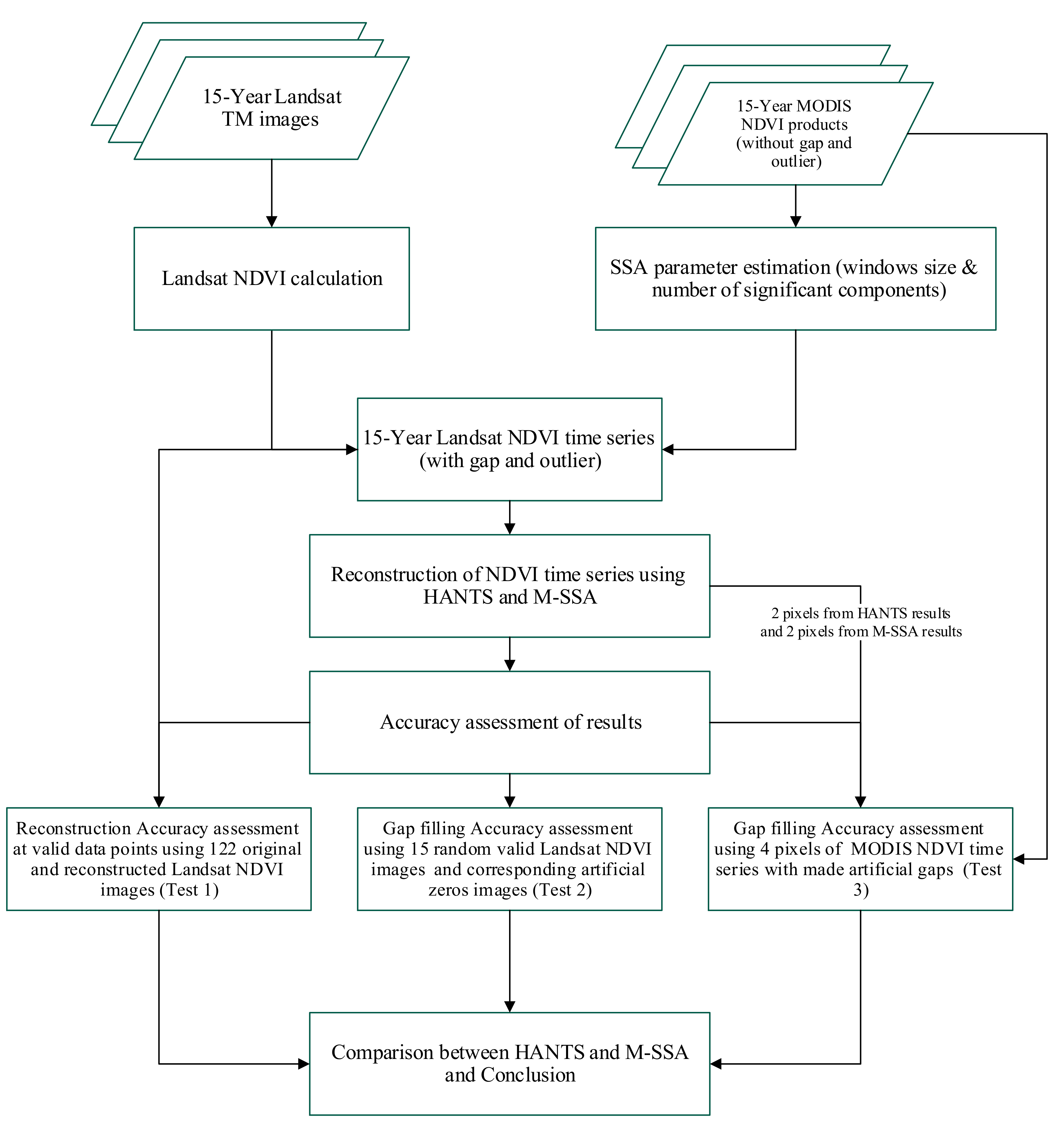
2.5. Research Method

The Landsat calculated NDVI time series was reconstructed using the HANTS and (M)-SSA algorithms. HANTS and SSA codes are accessible free of charge at https://www.mathworks.com/matlabcentral/fileexchange/38841-matlab-implementation-of-harmonic-analysis-of-time-series-hants and http://research.atmos.ucla.edu/tcd//ssa/form.html, respectively.

The algorithms and also resources limitations do not allow processing of the fifteen-year time series at the same time. The former limitation is due to HANTS code which only handles 19 frequencies (see Section 3.1) and the latter is due to the computer RAM and processor affecting the size of the original data to HANTS as well as (M-)SSA algorithms.

The limitation in the HANTS algorithm is addressed by splitting the 15 years in two. In order to get reliable results, the number of valid observations must be always being greater that the number of parameters required to describe the signal (2 × NOF + 1). Therefore, more data points than the necessary minimum should be included in the curve fitting procedure. In the results section, the processing of images and determination of the parameters of the HANTS algorithm are explained in detail.

The M-SSA limitation does not allow processing of the whole time series at once (1248 columns × 800 rows × 345 images). Therefore, the limitation is addressed splitting the original time series into 24 smaller blocks (208 columns × 200 rows × 345)

Each block was processed separately after which all blocks were finally put together. In order to enable reconstruction of the time series in M-SSA software the window size and number of significant components firstly need to be determined. Since the component’s calculation (SSA algorithm) requires a complete temporal series (i.e., without gaps), MODIS NDVI time series product (MOD13Q1) with the same time period as Landsat data was used. To this end, MODIS 16-day NDVI product with spatial resolution of 250 m in the study region was used to extract the NDVI changes along a pixel during period 2000–2015. The 15-year time series with 345 images of MODIS was used to identify the significant periodic components, the window size in SSA algorithm. These parameters were used to reconstruct the Landsat time series in M-SSA.

Using MODIS NDVI time series, the effect of number of components and window size on the reconstruction of this time series was investigated by SSA. Different statistical and mathematical tests in SSA software (e.g., Monte Carlo test) were then performed to determine whether a component is significant or not. After finding the window size and significant components, Landsat 5 TM NDVI time series were reconstructed by M-SSA algorithm.

Evaluation and Comparison of (M)-SSA and HANTS

Root Mean Square Error (RMSE) was used to evaluate the performance and accuracy of both algorithms for reconstruction of the images of this time series as follows:

$$\mathrm{RMSE}=\sqrt{\frac{{\displaystyle \sum _{i=1}^n{(x_i-y_i)}^2}}{n}}$$

(5)

In Equation (5), the original and reconstructed data were represented by x_i and y_i, respectively. Three different scenarios (tests) were created to show the capability of HANTS and (M)-SSA algorithms in reconstruction of NDVI time series. As the first test (Test 1), an RMSE map was prepared using the 122 existing Landsat NDVI images and 122 corresponding reconstructed images in HANTS and M-SSA algorithms pixel by pixel. The RMSE map prepared by this method is only indicative of the reconstruction capability of both algorithms at valid data points. Therefore, the gap filling capability at points with missing data cannot be estimated in this step.

In the second test (Test 2), to evaluate the gap filling capability of HANTS and M-SSA algorithms, among 122 primary original Landsat NDVI images, 15 images were randomly selected along a time series with no cloud observations. In total, 15 original images were extracted from the time series, and they were replaced by 15 images with zero data to be reconstructed by HANTS and M-SSA algorithms. A new time series which had 69% missing data (in average) was then reconstructed by both algorithms with the same parameters obtained in the results section. Using 15 existing images extracted from the time series and 15 corresponding reconstructed images by both algorithms, an RMSE map was prepared the same as the first method.

In the third test (Test 3), eight single time series (segments of 8 pixels in time) were used to analyze the ability of both algorithms in filling the gaps due to missing data in NDVI time series. Two time series from the reconstruction results of HANTS algorithm and two time series from the results of M-SSA algorithm were selected. To get more reliable results, further, four other 250-m resolution MODIS NDVI 16-day time series were selected in the study region. Missing data or gaps were then artificially created in these eight time series with the same distribution and dispersion as the missing data in original NDVI time series. These time series were then reconstructed by HANTS and M-SSA algorithms with the same parameters obtained in the results section. RMSEs between the reconstructed and original data were calculated to compare HANTS and M-SSA algorithms gap filling capability. The procedures used in this study are summarized by the flow chart in Figure 4.

3. Results and Discussion

3.1. Most Relevant Periodic Components for HANTS Algorithm

The more completely the time series is studied, the better the results of reconstruction will be. This is due to the fact that as the number of valid data increase, the degree of freedom for curve fitting will increase. In this regard, this time series can be processed and reconstructed as a fifteen-year time series with 345 images. As recommended earlier in Section 2.5, a maximum of 19 frequencies can be considered in HANTS software. In the studied 15-year time series, the base period was 345 considering the number of all images. When the base period was divided by the number of frequencies, the re-constructible period in this time series was obtained. Therefore, given the maximum number of frequencies in HANST software (at last 19) and 345 images in this fifteen-year time series, the shortest re-constructible period was an 18-image period (345.19 ≈ 18). However, in NDVI time series, annual and six-month periods are the dominant periods of NDVI changes, and these periods in 16-day NDVI time series appear almost as 23- and 12-image periods. Thus, if we use 345 images as the base period, the six-month periods cannot be reconstructed in this state, and the results will be unreliable. To eliminate this limitation in HANTS algorithm, this 15-year time series was processed and reconstructed as a 7- and an 8-year time series separately. As mentioned above, this is because the curve fitting procedure needs the maximum number of valid data (maximum degree of freedom) until the final result will be reliable.

Table 1. Parameters used in HANTS algorithm.

Type of Time Series		Base Period	Number of Frequencies	Shortest Period	Valid Data Range	Orientation of Outliers	FET	DOD	Duration of Processing
15-year time series	First 7-year time series	160	12	13 (≈6 months)	−1 to 1	low	0.02	5	13 min
	Second 8-year time series	182	14	13 (≈6 months)	−1 to 1	low	0.02	5	16 min

presents the parameters used in HANTS algorithm to reconstruct the 15-year NDVI time series. The valid data range was considered from -1 to 1 based on the acceptable range of NDVI. FET and DOD rates were considered to be 0.02 NDVI and 5. The base period was 169 images in the first 7-year time series and 182 images in the second 8-year time series. The number of frequencies was 12 in the first 7-year time series and 14 in the second 8-year time series. Here, the shortest period of reconstruction was 13 images, which was almost similar to a 6-year period. In Table 1, the duration of processing of each time series was compared with the SSA algorithm.

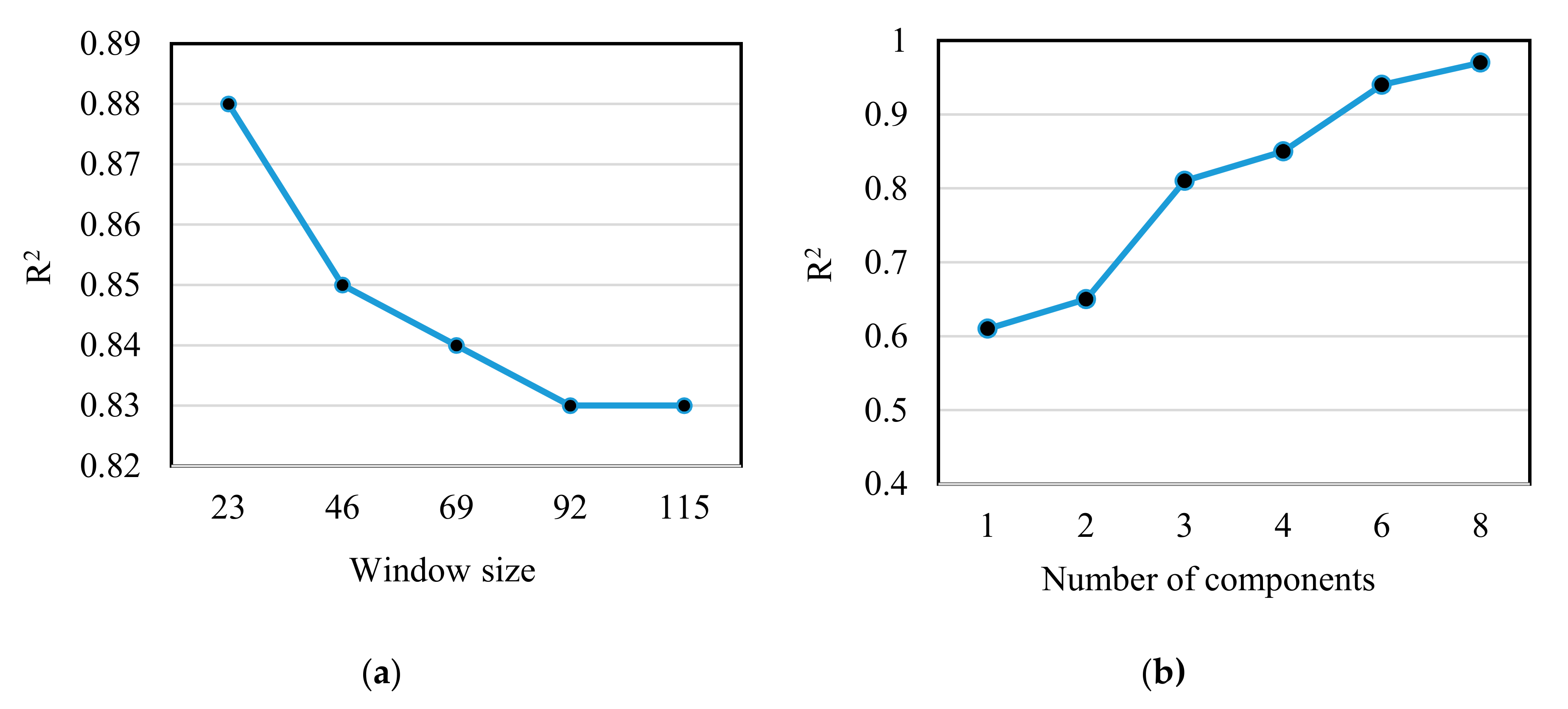
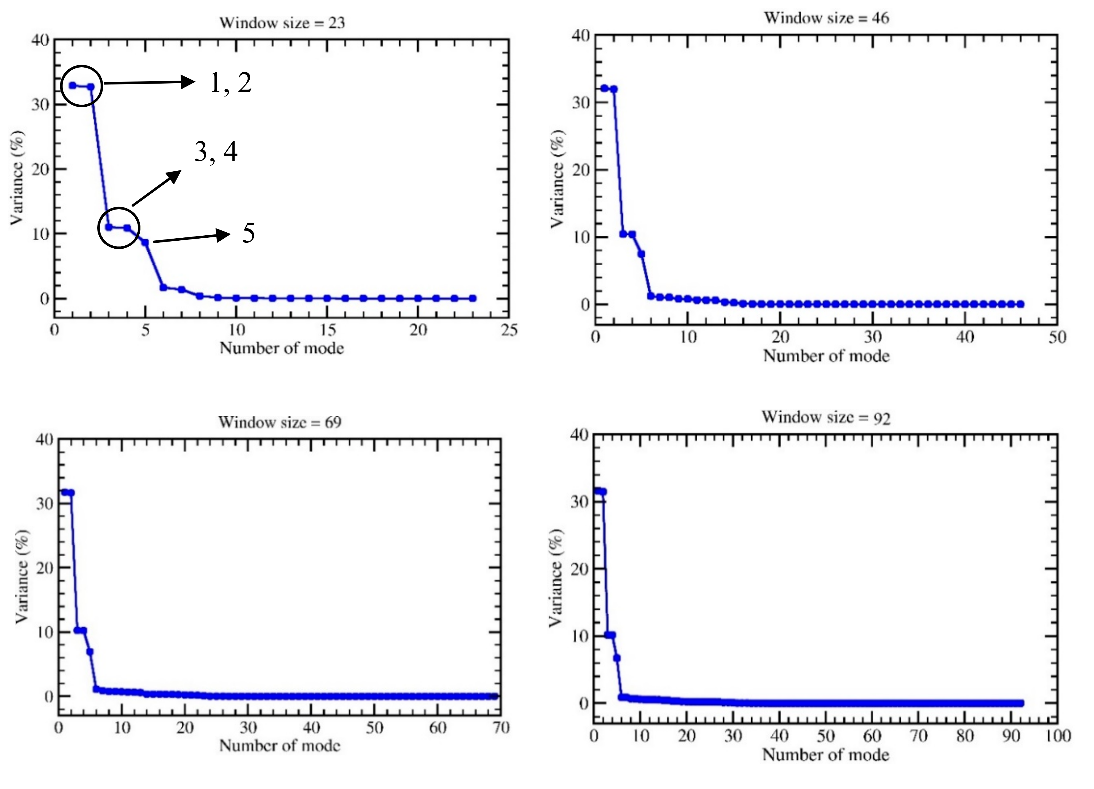
3.2. Window Size and Number of Components of NDVI Time Series in SSA

The number of significant components and window size are two major parameters in time series reconstruction by SSA algorithm. Thus, it is first necessary to choose an optimal window size and number of components. Figure 5 (right) displays the effects of the number of components on the window size of 46 (as two years NDVI data, 23 × 2 = 46) in reconstruction of a time series with 345 imagery data (MODIS time series). By increasing the number of components, R² value was increased between the original data and results of signal reconstruction by SSA algorithm. Components 1, 2, 3, 4 and 5 had the highest effect on reconstruction of this time series; more than 90% correlation was obtained by using these components. Figure 5a shows the effect of window size on reconstruction of the same time series with five components in different window sizes. By increasing the window size, R² value decreased between the original and reconstructed data by SSA algorithm but the computation time increased. Using window size of 23 in signal reconstruction where long-gap missing data exists, will not make accurate results. Use of larger window size not only increased the accuracy of reconstruction, but also decreased the time of processing; hence, in the present study, the time series was processed using a window size of 46. The accurate retrieval of the main components of a time series and window size by SSA algorithm tests are explained completely in the next sections.

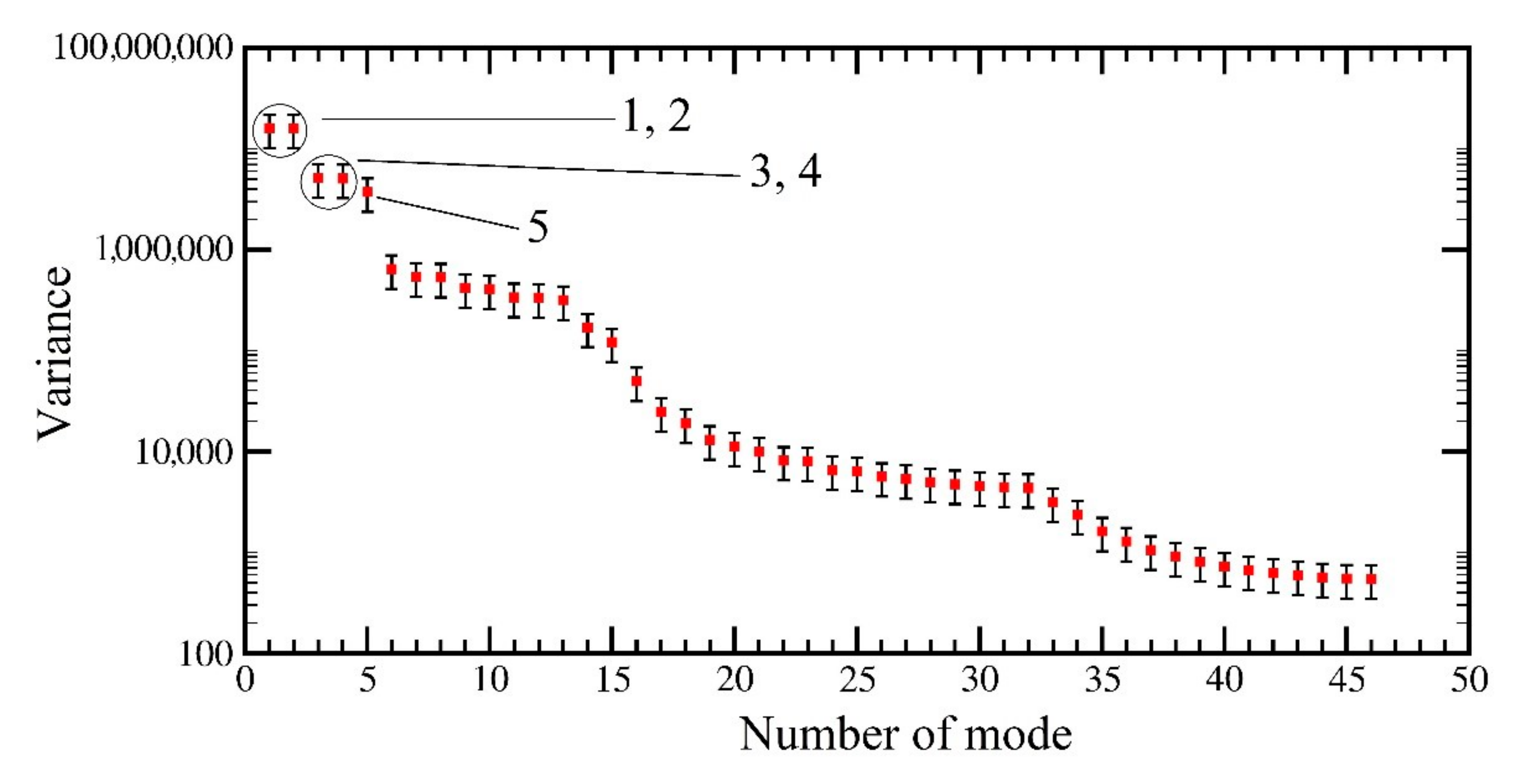
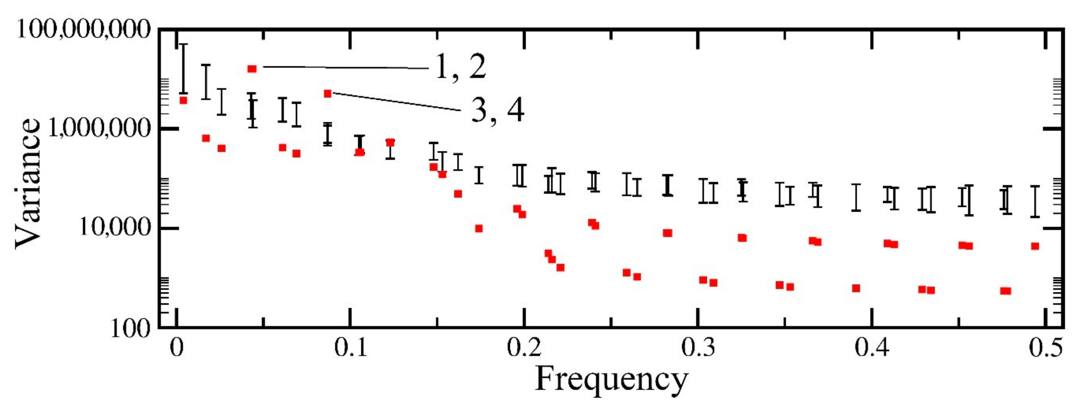
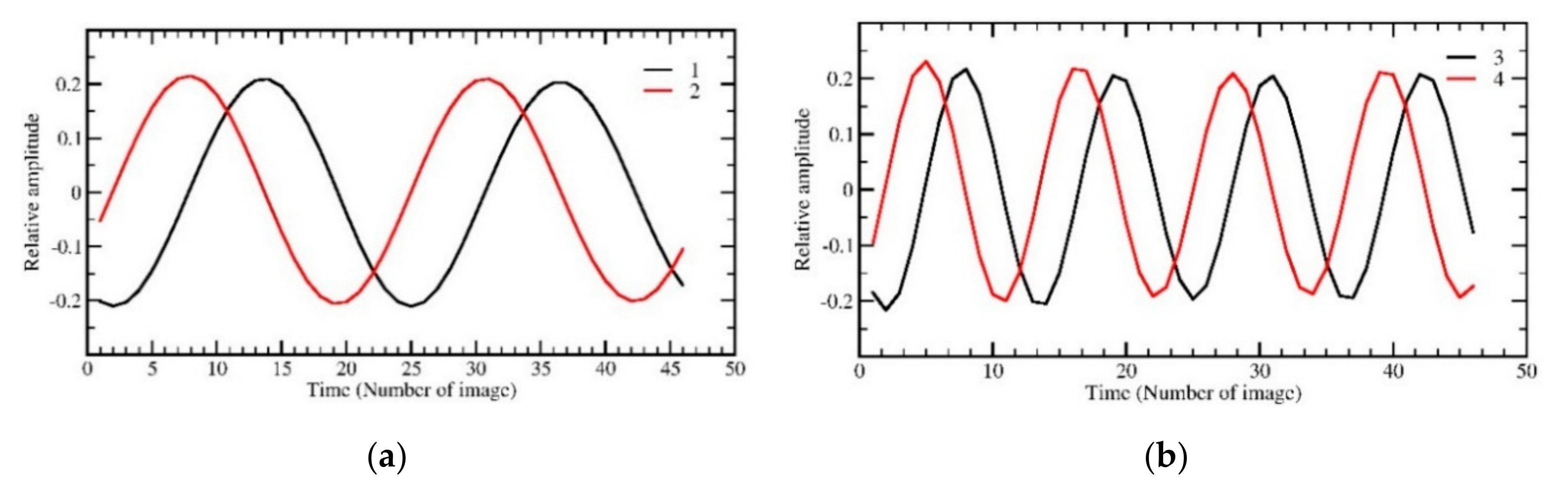
3.3. Most Significant Periodic Components for SSA

Eigenvalues obtained using a window size of 46 are shown in Figure 6. The eigenvalues plotted in decreasing order of variance values represent a sharp gradient for the first eigenvalues and it reduces to almost zero for the last eigenvalues. The sharp gradient shows the main components of the signal, and the low gradient (graph tail) shows the noise contained in the signal. There are 46 modes in the horizontal axis while the vertical axis shows the variance (i.e., eigenvalue). According to Figure 6, components 1, 2, 3, 4 and 5 significantly have the highest rate of variance (with 97.5% significant level). Components 1 and 2 as well as 3 and 4 are paired in the graph, so each pair effectively shows a periodic fluctuation in the time series [36]. When two components are paired equally, their empirical orthogonal functions are transferred in the quarter phase (phase difference). Therefore, these components show a similar periodic fluctuation with the phase difference. When, a component appears both significant and singular, it indicates a trend in the time series (i.e., component number 5 in Figure 6) [36].

Figure 7. shows the normalized eigenvalues in window sizes 23, 46, 69 and 92. As shown, with an increase in the number of windows, components 1, 2, 3, 4 and 5 are still the most important components of this time series, which have the highest variance. On the other hand, choosing different window sizes had a slight effect on increasing the reconstruction accuracy of this time series. Therefore, in the current research, the window size 46 was selected to reconstruct the time series. By choosing window size of 46, components 1 and 2 showed the highest variance in the signal so that 64% of variance was found for the components 1 and 2 (each with 32% variance). Components 3 and 4 showed 20% of variance and component 5 showed 7% of variance. In total, components 1–5, controlled 91% of variance in this time series. On the other hand, failure to choose these components to reconstruct this time series created a non-accurate signal, especially components 1, 2, 3 and 4, because, as shown, these components had the highest variance in this time series. These results were true for the window sizes 23, 69 and 92 (Figure 7).

3.4. Monte Carlo Test Results for Periodic Components

Figure 8 illustrates the results of Monte Carlo SSA test and shows the eigenvalues against their frequencies. As shown, components 1, 2, 3 and 4 are significant components (97.5%) of this time series. Components 1 and 2 as well as 3 and 4 overlap each other. The components are named by larger variance. The frequencies for components 1 and 2 as well as 3 and 4 are 0.0435 and 0.087, respectively. The reverse shows the frequency of the period. Therefore, the 23-image periods show 12 significant components of this time series.

Figure 9 depicts the temporal empirical orthogonal functions (T-EOFs) for the significant components of this time series based on the results of Monte Carlo test. The 23-image period in Monte Carlo test indicates the annual NDVI changes. As shown in Figure 9a, components 1 and 2 in each 23-image are repeated periodically with a lag of approximately 6 images. These two components have a phase difference of approximately six images. Based on Figure 9b, components 3 and 4 indicate the 12-image period, which are the phase difference of three images. The 12 16-day images show approximately six-month periods.

In general, the results of the Monte Carlo test showed that using window size of 46 yielded reliable results to reconstruct this time series. In the window size of 46, five significant components can be differentiated in this time series. Hence, five components and window size of 46 were used in M-SSA to reconstruct each of the 24 segments of this time series. The processing time of each segment in M-SSA algorithm was about 10 min, and the total time of processing of this time series was four hours.

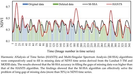
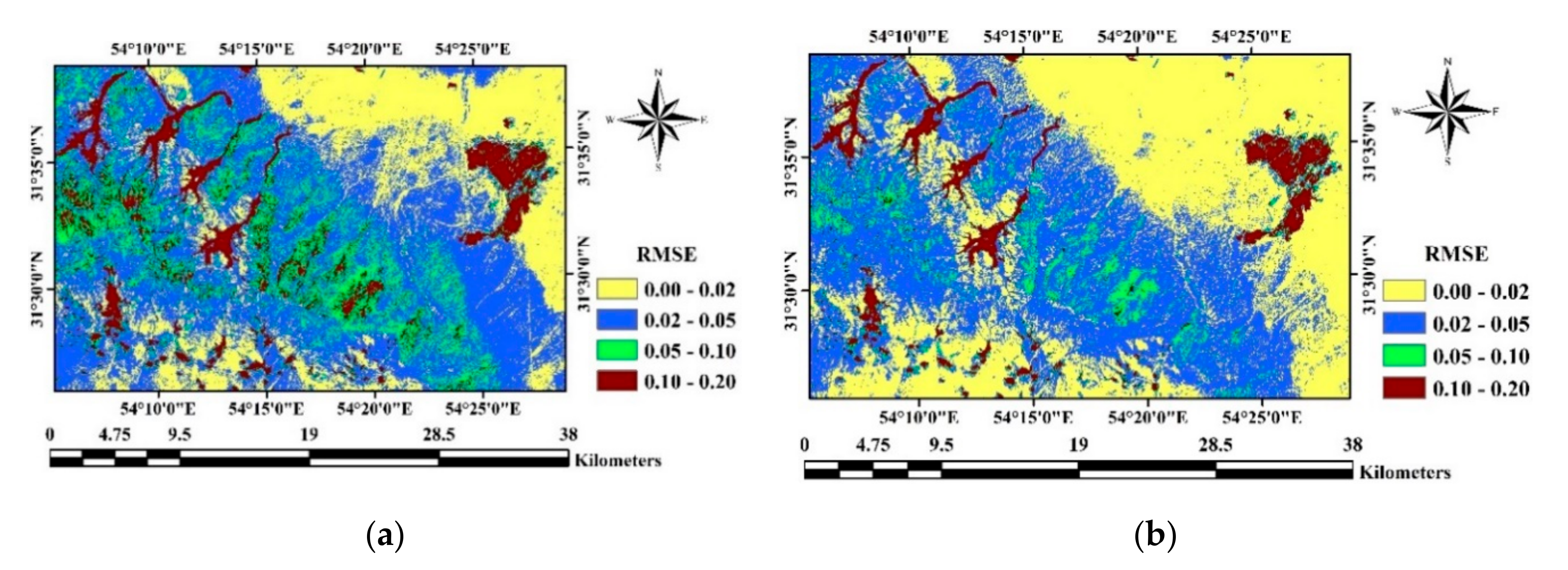
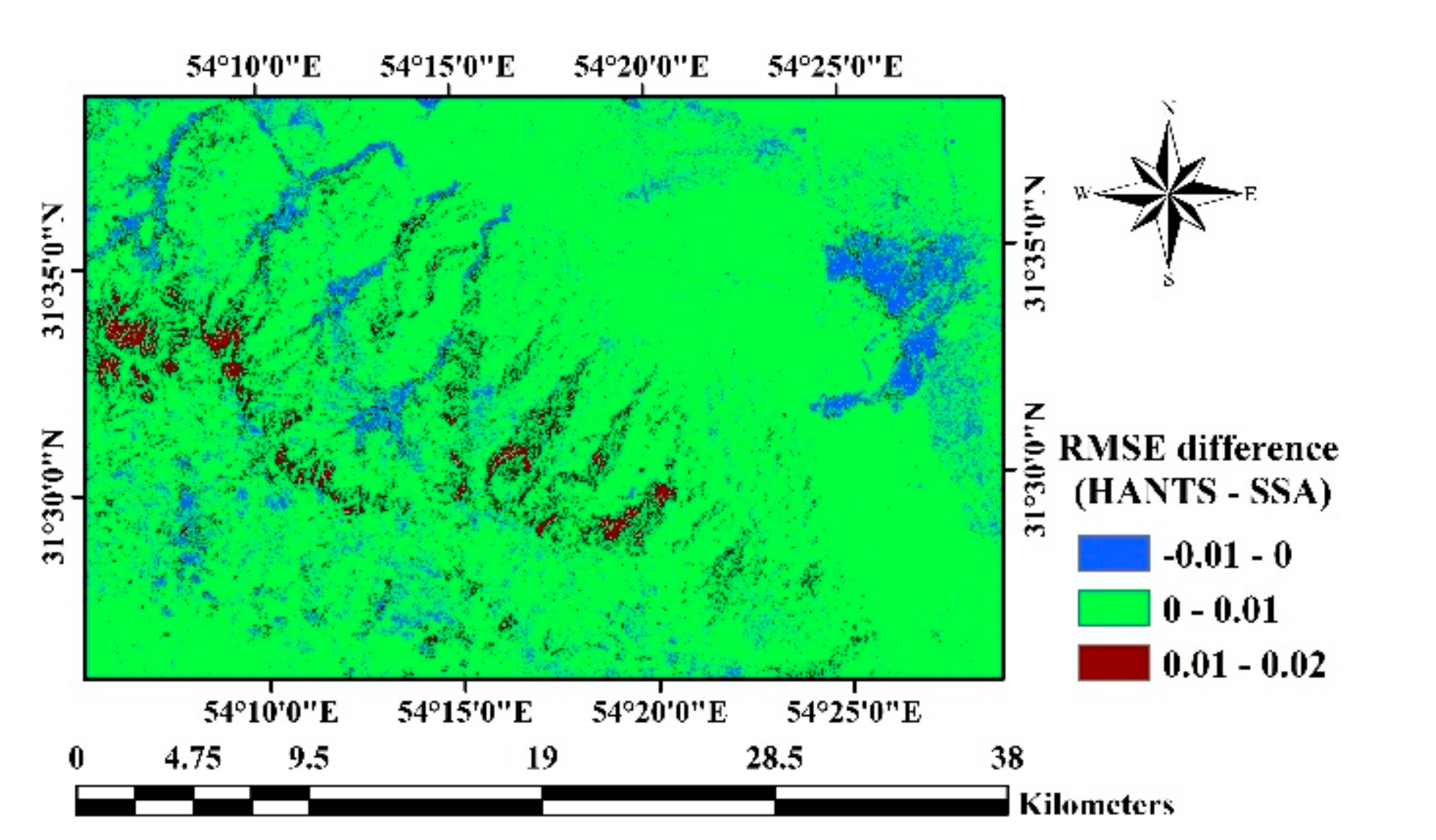
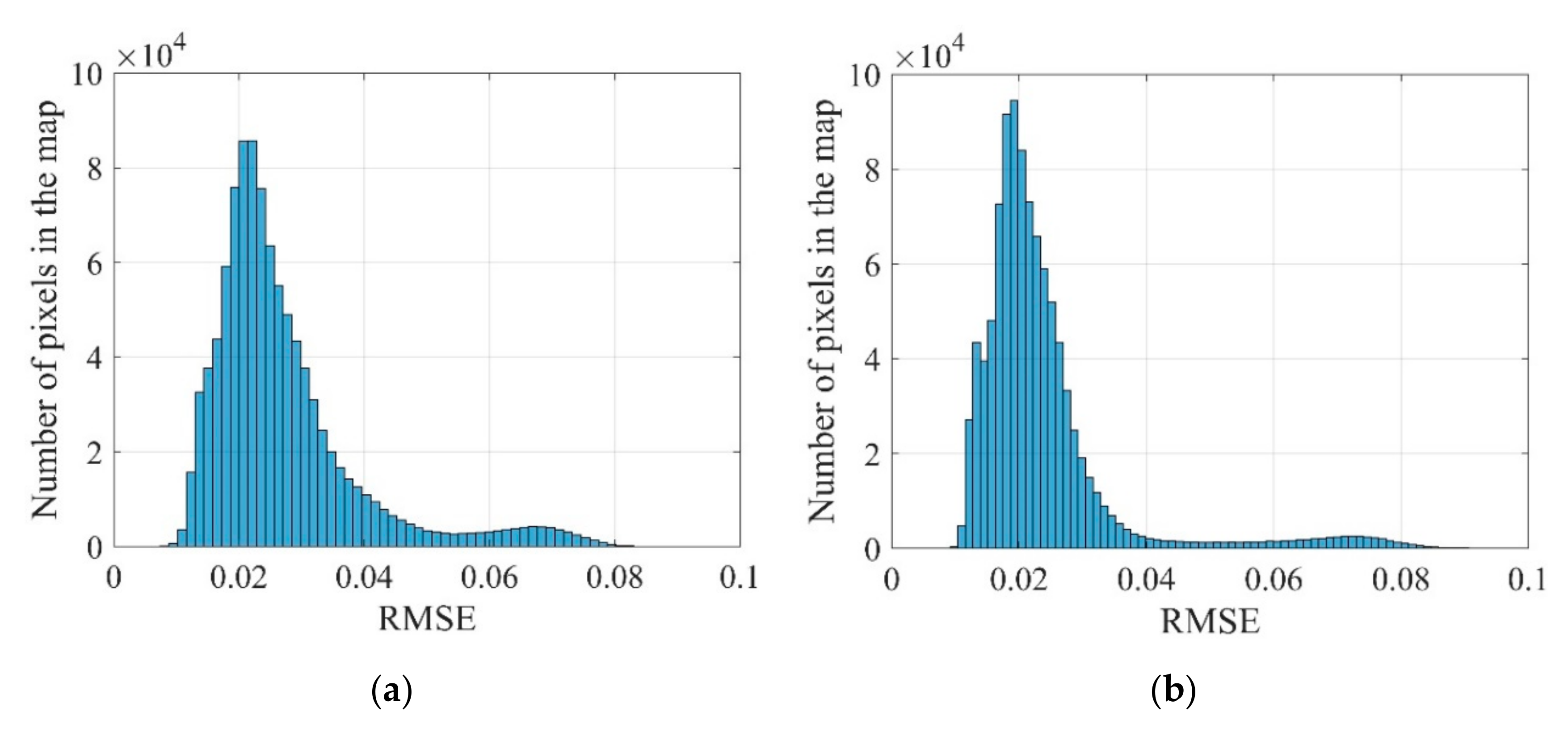
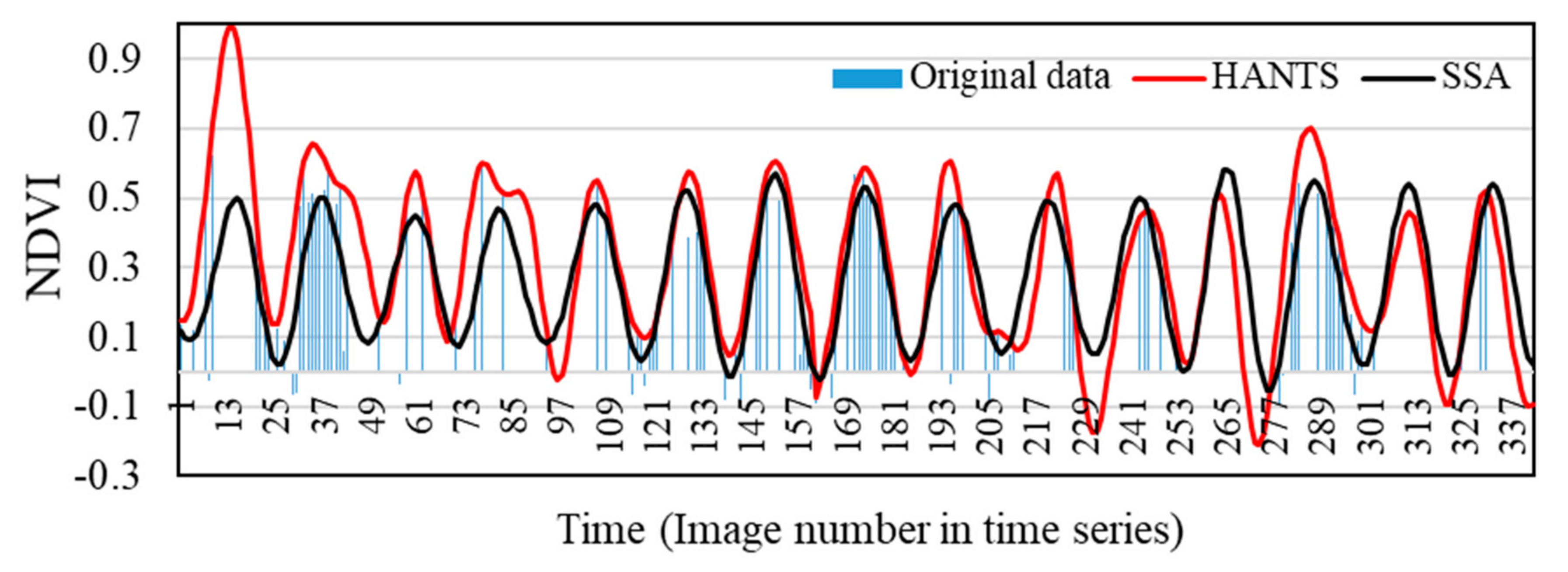
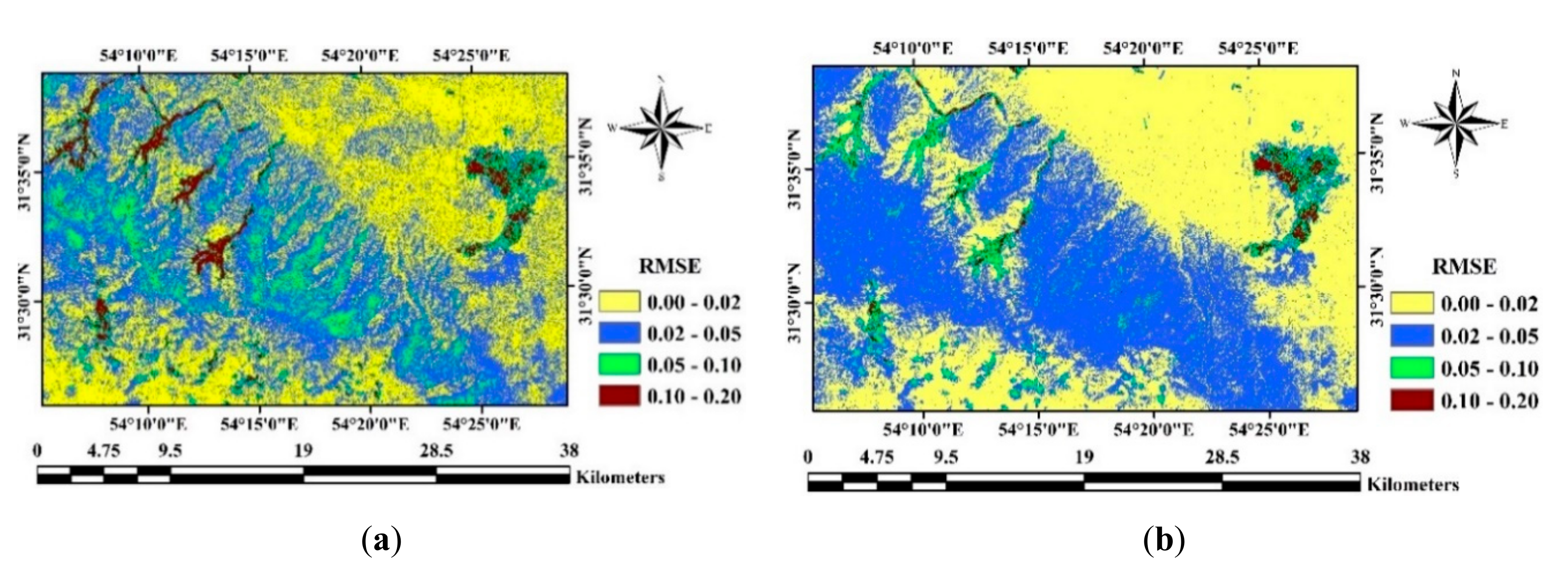
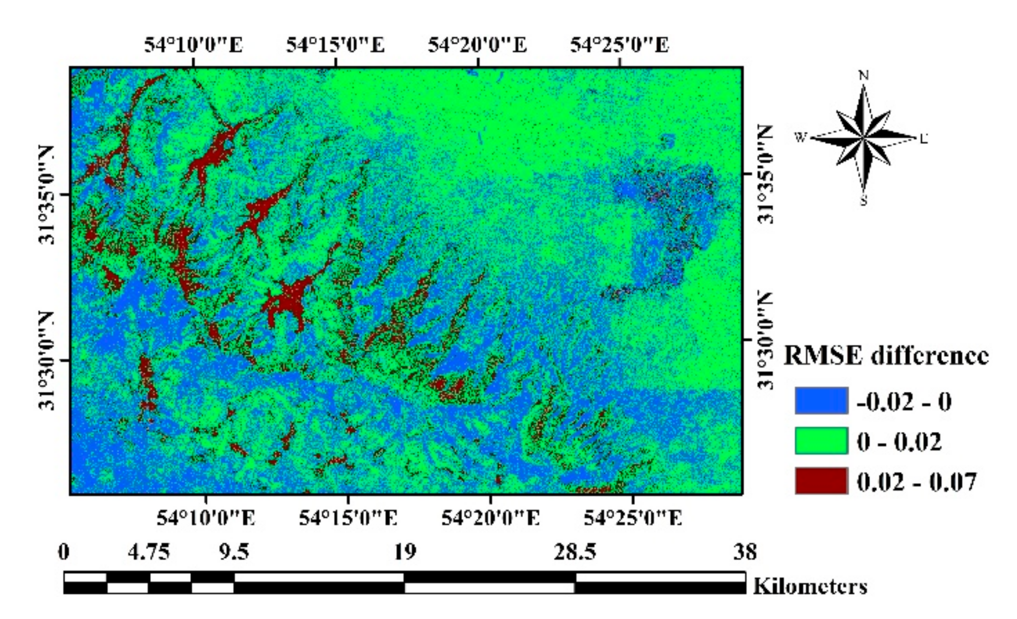
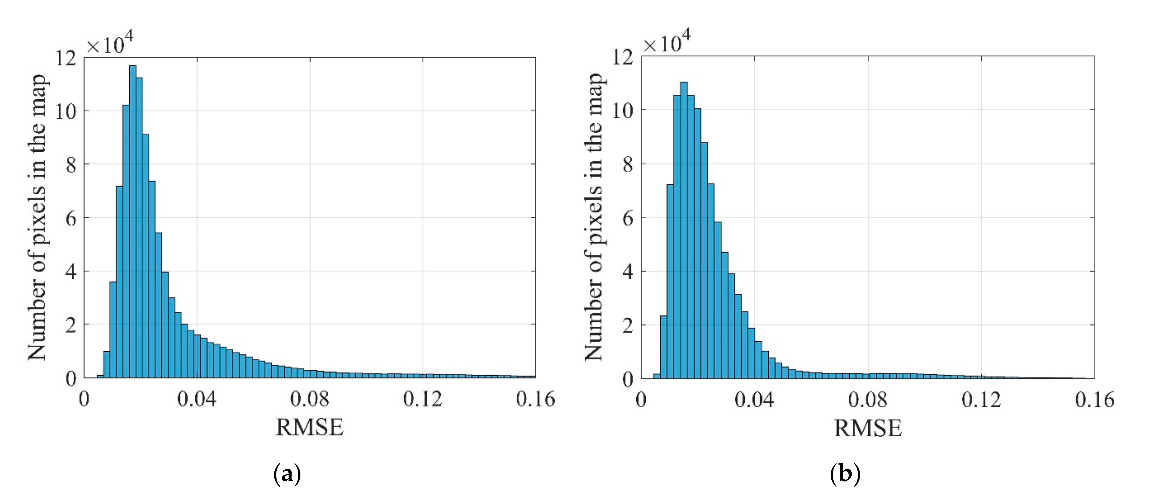
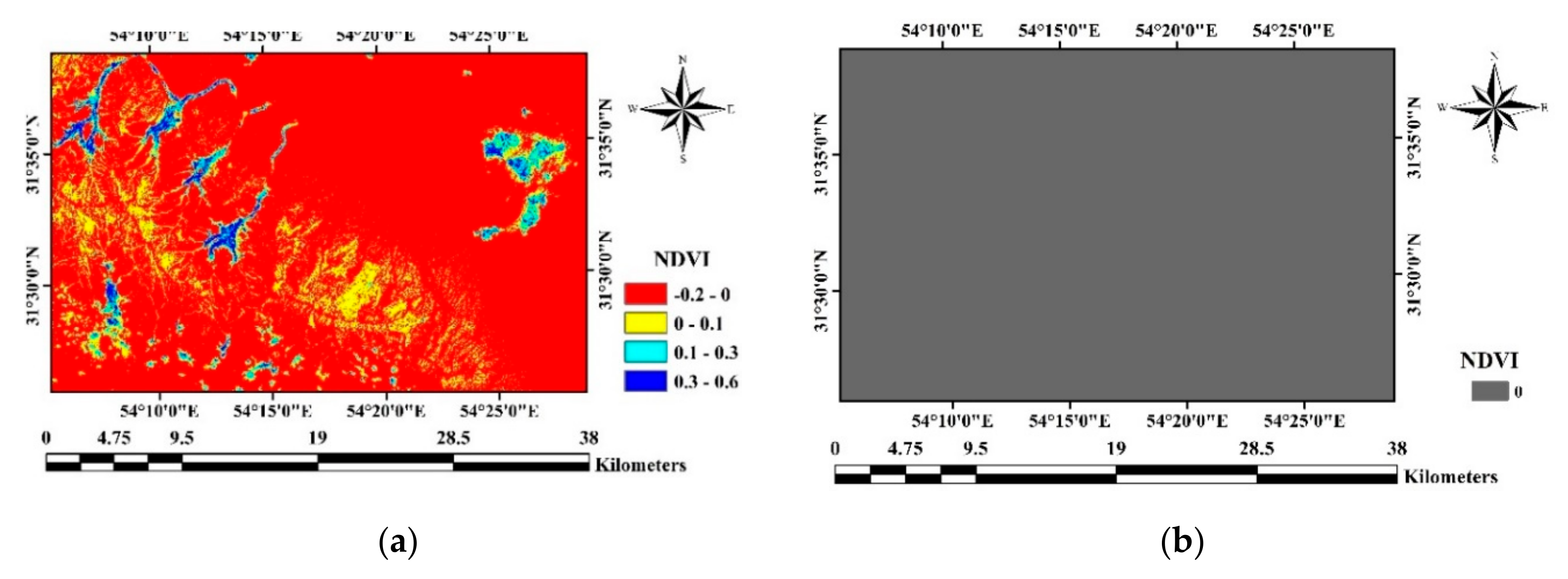
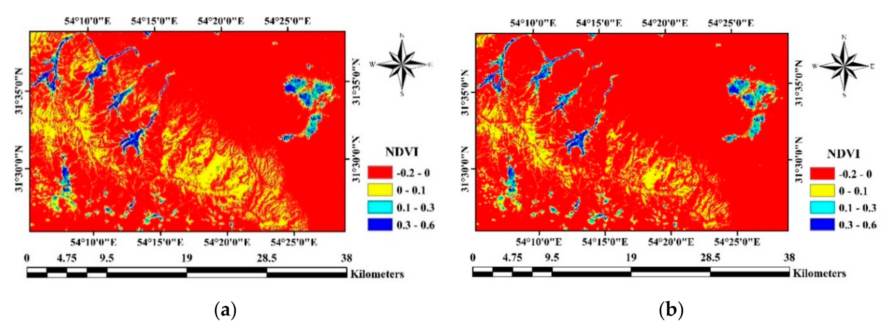
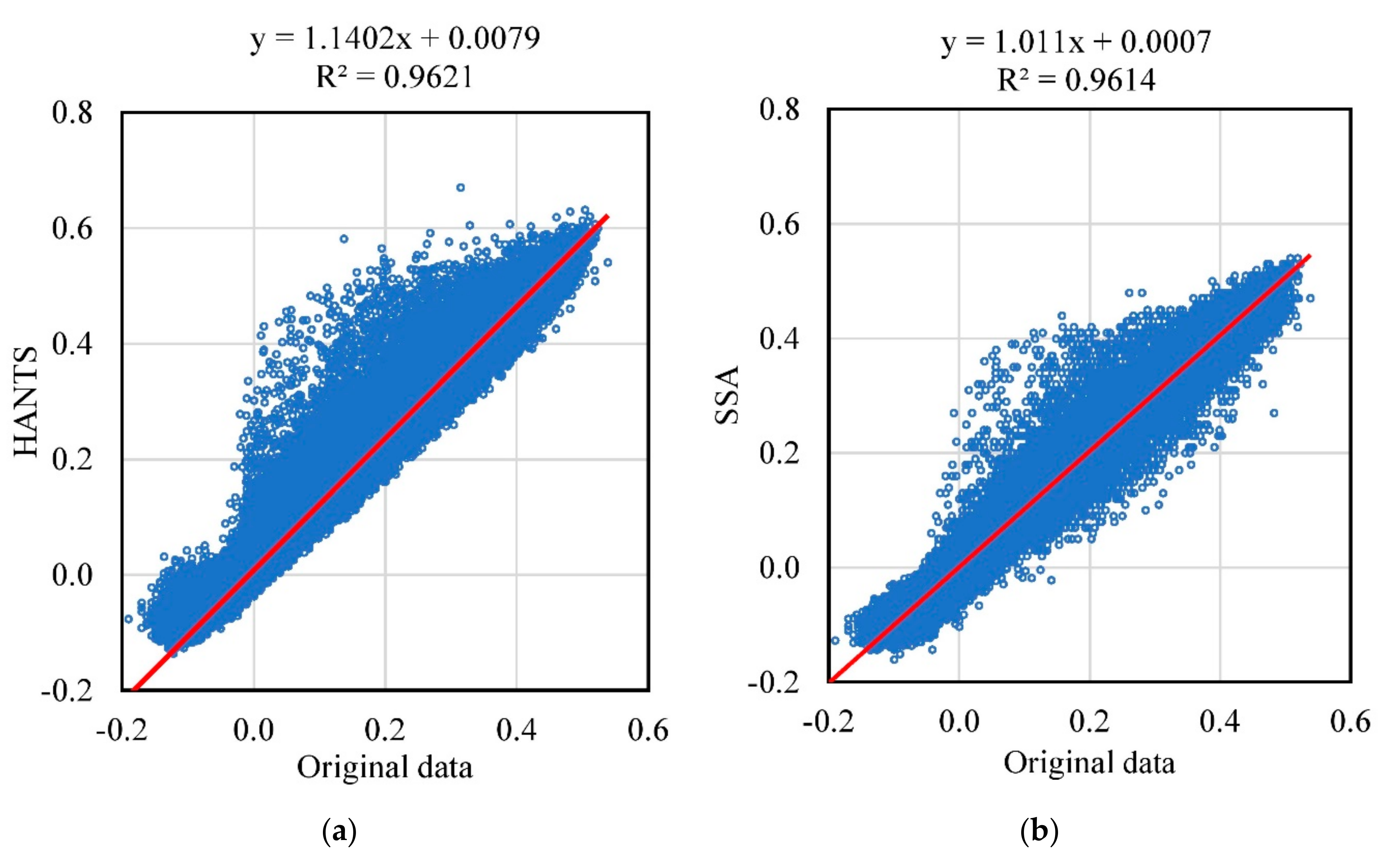
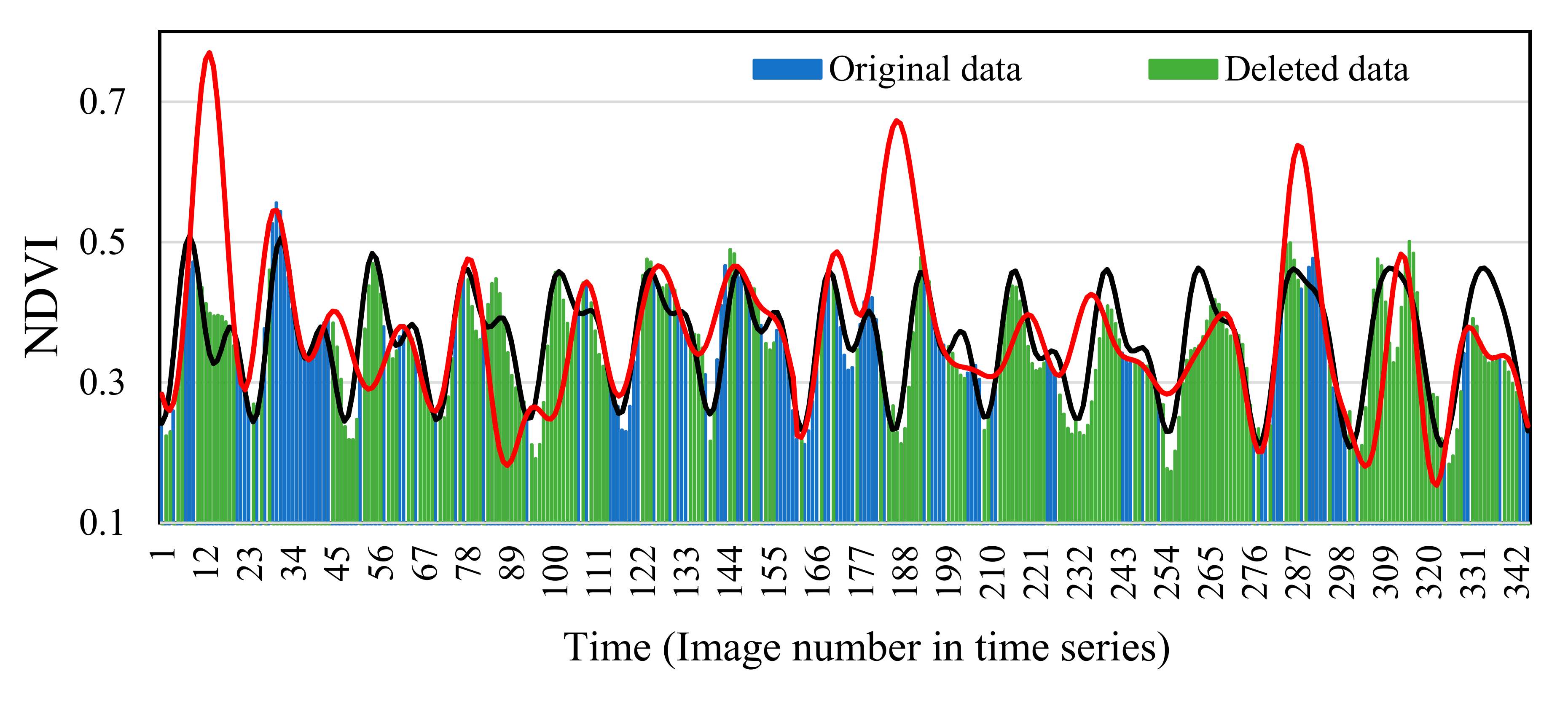
3.5. Assessment of Spatial and Temporal Reconstruction Accuracy

To illustrate the spatial accuracy of reconstruction (Test 1, see Section 2.5), Figure 10 depicts the RMSE map between the original and reconstructed data by HANTS and M-SSA algorithms in Landsat TM time series. As mentioned, there were only 122 images of this time series (out of 345 images). Therefore, RMSE maps in this mode were calculated from 122 images in the time series and reconstructed images by HANTS and M-SSA algorithms.

Figure 11 shows the RMSE map difference between HANTS and M-SSA. Based on the results, both algorithms have almost the same reconstruction accuracy. This concurs with Atkinson (2012) that a model does not always outperform others out rightly in all context as in this mode the performances did not differ much [19]. Although, the results of HANTS in mountain area where the probability of the clouds are more, the error has a slightly higher value (brown area in Figure 11).

The histograms of RMSE maps are shown in Figure 12. On average, RMSEs of the existing images and images reconstructed by HANTS and M-SSA algorithms were 0.027 and 0.023 NDVI, respectively. Figure 13 shows a time series along one pixel in the studied area and its reconstruction using HANTS and M-SSA algorithms. As shown, the signal fitted to the time series by the M-SSA algorithm is superior to the HANTS algorithm.

3.6. Assessment of Spatial and Temporal Gap-Filling Accuracy

Figure 14 shows the temporal gap-filling capability of HANTS and M-SSA based on Test 2 described in Section 2.5. The RMSE was mostly below 0.02 for reconstruction using M-SSA (right) algorithm while errors were largely higher using the HANTS algorithm (left). As indicated, the reconstruction error in M-SSA algorithm, the same as Figure 13, is less than that of the HANTS algorithm.

Figure 15 shows the RMSE difference map between HANTS and M-SSA. The results of HANTS in mountain area where the probability of the clouds is more, and the number of gaps are more, the error was a little higher than M-SSA (brown area in Fig15).

Figure 16 indicates the histogram of RMSE maps of 15 original images and 15 reconstructed images by HANTS and M-SSA algorithms. On average, the RMSEs of original NDVI images and images reconstructed by HANTS and M-SSA algorithms in this mode are 0.030 and 0.025.

Table 2. RMSE and R² between 15 random images extracted and reconstructed by the HANTS and M-SSA algorithms.

Date	HANTS		M-SSA
	RMSE	R2	RMSE	R2
1986/04/17	0.034	0.742	0.039	0.631
1987/09/11	0.020	0.962	0.015	0.961
1987/10/13	0.022	0.928	0.031	0.915
1988/03/21	0.083	0.181	0.033	0.649
1989/05/11	0.047	0.768	0.045	0.874
1990/08/18	0.030	0.866	0.022	0.945
1991/09/22	0.030	0.923	0.019	0.939
1992/07/06	0.026	0.928	0.025	0.930
1993/11/30	0.029	0.683	0.034	0.741
1994/07/28	0.022	0.949	0.018	0.936
1995/01/20	0.035	0.706	0.034	0.795
1996/08/18	0.040	0.887	0.024	0.924
1998/05/20	0.027	0.923	0.046	0.887
1998/10/27	0.020	0.906	0.030	0.896
2000/03/06	0.070	0.295	0.034	0.592
Mean	0.036	0.775	0.030	0.840

shows the dates, RMSE and R² between 15 random images extracted and reconstructed by the HANTS and M-SSA algorithms. According to Table 2, the M-SSA algorithm has a higher ability to fill the gaps than the HANTS algorithm. High R² indicate the closeness of the filled images to the observations. This is because, according to Table 2, on average, it has a smaller RMSE error and a higher correlation than the HANTS algorithm.

To indicate more about the accuracy of gap-filling spatially and temporally (Test 2), Figure 17 shows an example of 15 images extracted from the time series along with the image substituted with NaN (or zero) value (image 1987/09/11). The resulted obtained from HANTS and M-SSA algorithms for the image are shown in Figure 18. According to Figure 18 and spatial dispersion of NDVI classes, the reconstructed image by M-SSA algorithm is more compatible with the original image. Figure 19 indicates the results of correlation between the original images (Figure 17) and corresponding reconstructed images by HANTS and M-SSA algorithms (Figure 18, left and right, respectively). According to Figure 19, there is a high correlation in both algorithms so that R² value of the original and reconstructed images in both algorithms equals 0.96. However, the results of the M-SSA algorithm are more reliable because the gradient of the obtained equation is much close to 1. Although the RMSE has limitation of being easily driven to zero with sufficient parameters, in this case it indicated that M-SSA outperformed HANTS algorithm. The inclusion of other indicators of performance such as the Akaike Information Criterion (AIC) could further enhance the comparison [19].

Table 3. RMSE between original and reconstructed time series by M-SSA and HANTS using Landsat (Time series 1 to 4) and MODIS (Time series 5 to 8).

RMSE of Landsat Data			RMSE of MODIS Data
	M-SSA	HANTS		M-SSA	HANTS
Time series_1	0.02	0.04	Time series_5	0.046	0.087
Time series_2	0.048	0.12	Time series_6	0.041	0.1
Time series_3	0.102	0.023	Time series_7	0.052	0.102
Time series—4	0.112	0.017	Time series_8	0.045	0.117
Mean of RMSEs	0.071	0.05	Mean of RMSEs	0.046	0.102

presents RMSE values of reconstruction of eight different time series (single pixels) with artificial gaps (Test 3, see Section 2.5). As shown, in four time series made from the results, RMSEs mean in M-SSA and HANTS algorithms are 0.07 and 0.05. This presents a case where HANTS was superior to M-SSA in accuracy. In the four MODIS NDVI time series, the reconstruction error is significantly lower in the M-SSA algorithm than HANTS algorithm, 0.04 and 0.1, respectively. As an example, original MODIS NDVI time series 6_ together with deleted data and the results of both algorithms are shown in Figure 20. As indicated, the signal fitted by M-SSA algorithm has produced acceptable results at points with missing data compared to HANTS algorithm. However, in the HANTS algorithm, the fitted signal has yielded unacceptable results in the missing data in the time series in general.

Overall, the M-SSA algorithm which fills gaps using both the spatial and temporal components largely outperformed the HANTS which uses the temporal component alone. Other studies have also indicated the superiority of algorithms which use both the spatial and temporal components in reconstruction [16,18,19,57]. The findings showed that the M-SSA algorithm can effectively solve the problem of long-gap of missing data (more than 50% time series) in NDVI time series which was also confirmed by other studies [5,8,38,41]. Another limitation of HANTS algorithm is that signal reconstruction error is high when the gaps are at the beginning and end of the time series, especially when there is a long-term increasing or decreasing regular trend in a time series. This is because the HANTS algorithm reconstructs a time series based on periodic behavior. Further, the user should have adequate information about the periodic behavior of the time series under processing in HANTS algorithm, while the periodic behaviors and trends can be recognized in M-SSA algorithm.

4. Conclusions

In the present study, HANTS and M-SSA algorithms were comparatively used to fill in missing data of NDVI time series derived from the Landsat 5 TM and MODIS data. MODIS NDVI data were also used to extract periodic components and validate the results. The results showed that the M-SSA accuracy in filling the gaps of missing data was higher than that of the HANTS algorithm. HANTS has limitations in reconstruction of long-gap time series because a maximum of 19 frequencies can be considered in this software, whereas M-SSA software has no limitation in this regard. Trends can be considered in reconstruction of a time series in M-SSA algorithm. In general, M-SSA algorithm, in addition to reconstructing the remote-sensing time series, can be used to reconstruct other temporal time series in various scientific fields. In climatology it can be used to reconstruct the time series of daily temperature at meteorological stations and to extract the periods and climatic trends. In general, the findings showed that when the missing data in NDVI time series and other periodic time series are less than half of longer period (i.e., the main problems of time series are small gaps and outliers) HANTS algorithm can be used to reconstruct these time series. The higher the amount of missing data in a time series, the lower the accuracy of HANTS algorithm. Certainly, this algorithm can be used to reconstruct the time series with missing data less than 50%. Based on the type of time series and given the objectives and accuracy, each of these algorithms may have their own specific advantages. Furthermore, the results of the M-SSA algorithm can be used to solve the problem of missing data in Landsat 5 TM NDVI time series.

References

1. Ghafarian Malamiri, H.; Rousta, I.; Olafsson, H.; Zare, H.; Zhang, H. Gap-filling of MODIS Time Series Land Surface Temperature (LST) products using Singular Spectrum Analysis (SSA). Atmosphere 2018, 9, 334. [Google Scholar] [CrossRef] [Green Version]
2. Hosseini, S.Z.; Ghafarian Malamiri, H.R. Reconstruction of MODIS NDVI Time Series using Harmonic AN alysis of Time Series algorithm (HANTS). J. Spat. Plan. 2017, 21, 221–255. [Google Scholar]
3. Rousta, I.; Olafsson, H.; Moniruzzaman, M.; Ardö, J.; Zhang, H.; Mushore, T.D.; Shahin, S.; Azim, S. The 2000–2017 drought risk assessment of the western and southwestern basins in Iran. Modeling Earth Syst. Environ. 2020, 6, 1201–1221. [Google Scholar] [CrossRef]
4. Rousta, I.; Olafsson, H.; Moniruzzaman, M.; Zhang, H.; Liou, Y.-A.; Mushore, T.D.; Gupta, A. Impacts of drought on vegetation assessed by vegetation indices and meteorological factors in Afghanistan. Remote. Sens. 2020, 12, 2433. [Google Scholar] [CrossRef]
5. Ghafarian, H.R.; Menenti, M.; Jia, L.; den Ouden, H. Reconstruction of cloud-free time series satellite observations of land surface temperature. EARSel eProc. 2012, 11, 123–131. [Google Scholar]
6. Mobasheri, M.; Gholami, N.; Farajzadeh, A.M. Gradation of MODIS cloud mask algorithm using simultaneous aster imagery. J. Spat. Plan. 2011, 15, 81–99. (In Persian) [Google Scholar]
7. Menenti, M.; Ghafarian Malamiri, H.R.; Shang, H.; Alfieri, S.M.; Maffei, C.; Jia, L. Observing the response of terrestrial vegetation to climate variability across a range of time scales by time series analysis of land surface temperature. In Multitemporal Remote Sensing; Part of the Remote Sensing and Digital Image Processing Book Series; Springer: Amsterdam, The Netherlands, 2016; Volume 20, pp. 277–315. [Google Scholar]
8. Ghafarian Malamiri, H.R. Reconstruction of Gap-Free Time Series Satellite Observations of Land Surface Temperature to Model Spectral Soil Thermal Admittance. Ph.D. Thesis, Technische Universiteit Delft, Delft, The Netherlands, 2015. [Google Scholar]
9. Ackerman, S.A.; Strabala, K.I.; Menzel, W.P.; Frey, R.A.; Moeller, C.C.; Gumley, L.E. Discriminating clear sky from clouds with MODIS. J. Geophys. Res. Atmos. 1998, 103, 32141–32157. [Google Scholar] [CrossRef]
10. Rousta, I.; Sarif, M.O.; Gupta, R.D.; Olafsson, H.; Ranagalage, M.; Murayama, Y.; Zhang, H.; Mushore, T.D. Spatiotemporal analysis of land use/land cover and its effects on surface urban heat island using Landsat data: A case study of Metropolitan City Tehran (1988–2018). Sustainability 2018, 10, 4433. [Google Scholar] [CrossRef] [Green Version]
11. Sanaienejad, S.; Shah Tahmasbi, A.; Sadr Abadi Haghighi, R.; Kelarestani, K. A study of spectral reflection on wheat fields in Mashhad using MODIS data. JWSS Isfahan Univ. Technol. 2008, 12, 11–19. [Google Scholar]
12. Jia, L.; Shang, H.; Hu, G.; Menenti, M. Phenological response of vegetation to upstream river flow in the Heihe Rive basin by time series analysis of MODIS data. Hydrol. Earth Syst. Sci. 2011, 15, 1047–1064. [Google Scholar] [CrossRef] [Green Version]
13. Hird, J.N.; McDermid, G.J. Noise reduction of NDVI time series: An empirical comparison of selected techniques. Remote Sens. Environ. 2009, 113, 248–258. [Google Scholar] [CrossRef]
14. Roerink, G.; Menenti, M.; Verhoef, W. Reconstructing cloudfree NDVI composites using Fourier analysis of time series. Int. J. Remote Sens. 2000, 21, 1911–1917. [Google Scholar] [CrossRef]
15. Jonsson, P.; Eklundh, L. Seasonality extraction by function fitting to time-series of satellite sensor data. IEEE Trans. Geosci. Remote Sens. 2002, 40, 1824–1832. [Google Scholar] [CrossRef]
16. Beck, P.S.; Atzberger, C.; Høgda, K.A.; Johansen, B.; Skidmore, A.K. Improved monitoring of vegetation dynamics at very high latitudes: A new method using MODIS NDVI. Remote Sens. Environ. 2006, 100, 321–334. [Google Scholar] [CrossRef]
17. Chen, J.; Jönsson, P.; Tamura, M.; Gu, Z.; Matsushita, B.; Eklundh, L. A simple method for reconstructing a high-quality NDVI time-series data set based on the Savitzky–Golay filter. Remote Sens. Environ. 2004, 91, 332–344. [Google Scholar] [CrossRef]
18. Cao, R.; Chen, Y.; Shen, M.; Chen, J.; Zhou, J.; Wang, C.; Yang, W. A simple method to improve the quality of NDVI time-series data by integrating spatiotemporal information with the Savitzky-Golay filter. Remote Sens. Environ. 2018, 217, 244–257. [Google Scholar] [CrossRef]
19. Atkinson, P.M.; Jeganathan, C.; Dash, J.; Atzberger, C. Inter-comparison of four models for smoothing satellite sensor time-series data to estimate vegetation phenology. Remote Sens. Environ. 2012, 123, 400–417. [Google Scholar] [CrossRef]
20. Verhoef, W. Application of Harmonic Analysis of NDVI Time Series (HANTS); Dlo Winand Staring Center: Wageningen, The Netherlands, 1996; pp. 19–24. [Google Scholar]
21. Verhoef, W.; Menenti, M.; Azzali, S. Cover A colour composite of NOAA-AVHRR-NDVI based on time series analysis (1981–1992). Int. J. Remote Sens. 1996, 17, 231–235. [Google Scholar] [CrossRef]
22. Menenti, M.; Azzali, S.; Verhoef, W.; Van Swol, R. Mapping agroecological zones and time lag in vegetation growth by means of Fourier analysis of time series of NDVI images. Adv. Space Res. 1993, 13, 233–237. [Google Scholar] [CrossRef]
23. Zhou, J.; Jia, L.; Menenti, M. Reconstruction of global MODIS NDVI time series: Performance of harmonic analysis of time series (HANTS). Remote Sens. Environ. 2015, 163, 217–228. [Google Scholar] [CrossRef]
24. Jiang, X.; Wang, D.; Tang, L.; Hu, J.; Xi, X. Analysing the vegetation cover variation of China from AVHRR-NDVI data. Int. J. Remote Sens. 2008, 29, 5301–5311. [Google Scholar] [CrossRef]
25. Broomhead, D.; King, G.P. On the qualitative analysis of experimental dynamical systems. Nonlinear Phenom. Chaos 1986, 113, 114. [Google Scholar]
26. Broomhead, D.S.; King, G.P. Extracting qualitative dynamics from experimental data. Phys. D Nonlinear Phenom. 1986, 20, 217–236. [Google Scholar] [CrossRef]
27. Broomhead, D.; Jones, R.; King, G.; Pike, E. Singular system analysis with application to dynamical systems. In Choas, Noise and Fractals; Pike, E.R., Lugiato, L.A., Eds.; Malvern Physics Series; Adam Hilger: Bristol, UK, 1987; pp. 15–27. [Google Scholar]
28. Allen, M.R.; Smith, L.A. Monte Carlo SSA: Detecting irregular oscillations in the presence of colored noise. J. Clim. 1996, 9, 3373–3404. [Google Scholar] [CrossRef]
29. Danilov, D.; Zhigljavsky, A. Principal Components of Time Series: The ‘Caterpillar’ Method; University of St. Petersburg: Saint Petersburg, Russia, 1997; pp. 1–307. [Google Scholar]
30. Ghil, M.; Taricco, C. Advanced spectral analysis methods. In Past and Present Variability of the Solar-Terrestrial System: Measurement, Data Analysis and Theoretical Models; Ios Press: Amsterdam, The Netherlands, 1997; pp. 137–159. [Google Scholar]
31. Vautard, R.; Yiou, P.; Ghil, M. Singular-spectrum analysis: A toolkit for short, noisy chaotic signals. Phys. D Nonlinear Phenom. 1992, 58, 95–126. [Google Scholar] [CrossRef]
32. Yiou, P.; Sornette, D.; Ghil, M. Data-adaptive wavelets and multi-scale singular-spectrum analysis. Phys. D Nonlinear Phenom. 2000, 142, 254–290. [Google Scholar] [CrossRef] [Green Version]
33. Golyandina, N.; Nekrutkin, V.; Zhigljavsky, A.A. Analysis of Time Series Structure: SSA and Related Techniques; Chapman and Hall/CRC: Washington, DC, USA, 2001. [Google Scholar]
34. Jolliffe, I. Principal component analysis. In International Encyclopedia of Statistical Science; Springer: Berlin/Heidelberg, Germany, 2011; pp. 1094–1096. [Google Scholar]
35. Vautard, R.; Ghil, M. Singular spectrum analysis in nonlinear dynamics, with applications to paleoclimatic time series. Phys. D Nonlinear Phenom. 1989, 35, 395–424. [Google Scholar] [CrossRef]
36. Ghil, M.; Vautard, R. Interdecadal oscillations and the warming trend in global temperature time series. Nature 1991, 350, 324. [Google Scholar] [CrossRef]
37. Yiou, P.; Baert, E.; Loutre, M.-F. Spectral analysis of climate data. Surv. Geophys. 1996, 17, 619–663. [Google Scholar] [CrossRef]
38. Chen, Q.; van Dam, T.; Sneeuw, N.; Collilieux, X.; Weigelt, M.; Rebischung, P. Singular spectrum analysis for modeling seasonal signals from GPS time series. J. Geodyn. 2013, 72, 25–35. [Google Scholar] [CrossRef]
39. Kondrashov, D.; Ghil, M. Spatio-temporal filling of missing points in geophysical data sets. Nonlinear Process. Geophys. 2006, 13, 151–159. [Google Scholar] [CrossRef] [Green Version]
40. Kondrashov, D.; Shprits, Y.; Ghil, M. Gap filling of solar wind data by singular spectrum analysis. Geophys. Res. Lett. 2010, 37. [Google Scholar] [CrossRef] [Green Version]
41. Wang, D.; Liang, S. Singular spectrum analysis for filling gaps and reducing uncertainties of MODIS land products. In Proceedings of the IGARSS 2008—2008 IEEE International Geoscience & Remote Sensing Symposium, Boston, MA, USA, 7–11 July 2008; pp. V-558–V-561. [Google Scholar]
42. Rousta, I.; Doostkamian, M.; Haghighi, E.; Malamiri, H.R.G.; Yarahmadi, P. Analysis of spatial autocorrelation patterns of heavy and super-heavy rainfall in Iran. Adv. Atmos. Sci. 2017, 34, 1069–1081. [Google Scholar] [CrossRef]
43. Rousta, I.; Doostkamian, M.; Taherian, A.M.; Haghighi, E.; Ghafarian Malamiri, H.R.; Ólafsson, H. Investigation of the spatio-temporal variations in atmosphere thickness pattern of Iran and the Middle East with special focus on precipitation in Iran. Climate 2017, 5, 82. [Google Scholar] [CrossRef] [Green Version]
44. Rousta, I.; Javadizadeh, F.; Dargahian, F.; Olafsson, H.; Shiri-Karimvandi, A.; Vahedinejad, S.H.; Doostkamian, M.; Monroy Vargas, E.R.; Asadolahi, A. Investigation of vorticity during prevalent winter precipitation in Iran. Adv. Meteorol. 2018, 2018. [Google Scholar] [CrossRef] [Green Version]
45. Rousta, I.; Khosh Akhlagh, F.; Soltani, M.; Modir Taheri Sh, S. Assessment of blocking effects on rainfall in northwestern Iran. In Proceedings of the COMECAP, Heraklion, Greece, 28–31 May 2014; pp. 127–132. [Google Scholar]
46. Rousta, I.; Nasserzadeh, M.H.; Jalali, M.; Haghighi, E.; Ólafsson, H.; Ashrafi, S.; Doostkamian, M.; Ghasemi, A. Decadal spatial-temporal variations in the spatial pattern of anomalies of extreme precipitation thresholds (Case Study: Northwest Iran). Atmosphere 2017, 8, 135. [Google Scholar] [CrossRef] [Green Version]
47. Sabziparvar, A.A.; Mir Mousavi, S.H.; Karampour, M.; Doostkamian, M.; Haghighi, E.; Rousta, I.; Olafsson, H.; Sarif, M.O.; Gupta, R.D.; Moniruzzaman, M. Harmonic analysis of the spatiotemporal pattern of thunderstorms in Iran (1961–2010). Adv. Meteorol. 2019, 2019. [Google Scholar] [CrossRef] [Green Version]
48. Loveland, T.R.; Dwyer, J.L. Landsat: Building a strong future. Remote Sens. Environ. 2012, 122, 22–29. [Google Scholar] [CrossRef]
49. Tucker, C.J. Red and photographic infrared linear combinations for monitoring vegetation. Remote Sens. Environ. 1979, 8, 127–150. [Google Scholar] [CrossRef] [Green Version]
50. Verhoef, W. Application of harmonic analysis of NDVI time series (HANTS). In Fourier Analysis of Temporal NDVI in the Southern African and American Continents; Report 108; SC-DLO: Wageningen, The Netherlands, 1996; pp. 19–24. [Google Scholar]
51. Musial, J.P.; Verstraete, M.M.; Gobron, N. Comparing the effectiveness of recent algorithms to fill and smooth incomplete and noisy time series. Atmos. Chem. Phys. 2011, 11, 7905–7923. [Google Scholar] [CrossRef] [Green Version]
52. Izquierdo Verdiguier, E. Kernel Feature Extraction Methods for Remote Sensing Data Analysis; University of Valencia: Valencia, Spain, 2014. [Google Scholar]
53. Li, J.; Carlson, B.E.; Lacis, A.A. Application of spectral analysis techniques in the intercomparison of aerosol data: 1. An EOF approach to analyze the spatial-temporal variability of aerosol optical depth using multiple remote sensing data sets. J. Geophys. Res. Atmos. 2013, 118, 8640–8648. [Google Scholar] [CrossRef]
54. Elsner, J.B.; Tsonis, A.A. Singular Spectrum Analysis: A New Tool in Time Series Analysis; Springer Science & Business Media: New York, NY, USA, 2013. [Google Scholar]
55. Ghil, M.; Allen, M.; Dettinger, M.; Ide, K.; Kondrashov, D.; Mann, M.; Robertson, A.W.; Saunders, A.; Tian, Y.; Varadi, F. Advanced spectral methods for climatic time series. Rev. Geophys. 2002, 40. [Google Scholar] [CrossRef] [Green Version]
56. Schoellhamer, D.H. Singular spectrum analysis for time series with missing data. Geophys. Res. Lett. 2001, 28, 3187–3190. [Google Scholar] [CrossRef] [Green Version]
57. Yan, L.; Roy, D.P. Spatially and temporally complete Landsat reflectance time series modelling: The fill-and-fit approach. Remote Sens. Environ. 2020, 241, 111718. [Google Scholar] [CrossRef]
Figure 1. Location of study region in Iran and Yazd province.
Remotesensing 12 02747 g001
Figure 2. Distribution and dispersion of unavailable and available NDVI time series images of this study.
Remotesensing 12 02747 g002
Figure 3. Arrangement of studied time-series images (top) and NDVI changes on a pixel along with the missing data (bottom).
Remotesensing 12 02747 g003
Figure 4. Flow chart of the main processes of this study.
Remotesensing 12 02747 g004
Figure 5. R2 values between the original data and reconstructed data by SSA in a time series with 345 pieces of data for different window sizes (a) and for different number of components (b).
Remotesensing 12 02747 g005
Figure 6. Singular values spectrum of data with window size of 46 image with five modes.
Remotesensing 12 02747 g006
Figure 7. Normalized singular values with 23, 46, 69 and 92 image window size.
Remotesensing 12 02747 g007
Figure 8. Monte Carlo SSA based on data EOFs test.
Remotesensing 12 02747 g008
Figure 9. SSA T-EOFs of components 1–2 (a), and 3–4 (b).
Remotesensing 12 02747 g009
Figure 10. RMSE map between the original and reconstructed time series using the HANTS algorithm (a) and the M-SSA algorithm (b).
Remotesensing 12 02747 g010
Figure 11. Difference between RMSE map of HANTS and M-SSA. Positive values show that the RMSE in HANTS is higher than M-SSA and vis versa.
Remotesensing 12 02747 g011
Figure 12. RMSE histogram using the HANTS algorithm (a) and the M-SSA algorithm (b).
Remotesensing 12 02747 g012
Figure 13. Original and reconstructed data signal using HANTS and M-SSA algorithms on NDVI time series for one pixel.
Remotesensing 12 02747 g013
Figure 14. RMSE map of 15 original images extracted from the time series and reconstructed by HANTS algorithm (a) and M-SSA algorithm (b).
Remotesensing 12 02747 g014
Figure 15. Difference between RMSE map of HANTS and M-SSA. Positive values show that the RMSE in HANTS is higher than M-SSA and vis versa.
Remotesensing 12 02747 g015
Figure 16. Histogram of 15 original images extracted from the time series and reconstructed by HANTS algorithm (a) and SSA algorithm (b).
Remotesensing 12 02747 g016
Figure 17. An image extracted from the time series (a) and NaN (or zero) value image (b).
Remotesensing 12 02747 g017
Figure 18. Reconstructed image by HANTS algorithm (a) and M-SSA algorithm (b).
Remotesensing 12 02747 g018
Figure 19. Correlation of original image with reconstructed image in HANTS algorithm (a) and M-SSA algorithm (b).
Remotesensing 12 02747 g019
Figure 20. Original MODIS NDVI time series along with deleted data and reconstruction using HANTS (red line) and M-SSA (black line) algorithms.
Remotesensing 12 02747 g020