Abstract
Snow is one of the essential factors in hydrology, freshwater resources, irrigation, travel, pastimes, floods, avalanches, and vegetation. In this study, the snow cover of the northern and southern slopes of Alborz Mountains in Iran was investigated by considering two issues: (1) Estimating the snow cover area and the (2) effects of droughts on snow cover. The snow cover data were monitored by images obtained from the Moderate Resolution Imaging Spectroradiometer (MODIS) sensor. The meteorological data (including the precipitation, minimum and maximum temperature, global solar radiation, relative humidity, and wind velocity) were prepared by a combination of National Centers for Environmental Prediction-Climate Forecast System Reanalysis (NCEP-CFSR) points and meteorological stations. The data scale was monthly and belonged to the 2000–2014 period. In the first part of the study, snow cover estimation was conducted by Multiple Linear Regression (MLR), Least Square Support Vector Machine (LSSVM), Group Method of Data Handling (GMDH), Multilayer Perceptron (MLP), and MLP with Grey Wolf Optimization (MLP-GWO) models. The most accurate estimations were produced by the MLP-GWO and GMDH models. The models produced better snow cover estimations for the northern slope compared to the southern slope. The GWO improved the MLP’s accuracy by 10.7%. In the second part, seven drought indices, including the Palmer Drought Severity Index (PDSI), Bahlme–Mooley Drought Index (BMDI), Standardized Precipitation Index (SPI), Multivariate Standardized Precipitation Index (MSPI), Modified Standardized Precipitation Index (SPImod), Joint Deficit Index (JDI), and Standardized Precipitation-Evapotranspiration Index (SPEI) were calculated for both slopes. The results showed that the effects of a drought event on the snow cover area would remain up to 5 (or 6) months in the region. The highest impact of drought appears after two months in the snow cover area, and the drought index most related to snow cover variations is the 2–month time window of SPI (SPI2). The results of both subjects were promising and the methods can be examined in other snowy areas of the world.
1. Introduction
Snow cover in many regions around the world has a direct impact on human life, including engineering, irrigation, travel, recreation, and hydrology. Additionally, floods and avalanches are important natural hazards, which are strongly associated with snow [1]. Another major aspect of snow is its interaction with vegetation. The melting of this water source contributes to vegetation survival and fertility, and has a profound effect on the phenomenon of soil frost and plant chilling injury [2,3,4].
The snow cover area is one of the most important parameters of the hydrological and climate cycles. Field measurements can provide clues for observable changes in much of our knowledge on the cryosphere. Over the last 20 years, due to the lack of appropriate accessibility, the influence of various topographic and physiographic features on the estimation of cryosphere hydrological parameters, and the insufficiency of meteorological stations at a high altitude have made the necessity of using indirect methods more prominent at regional and global scales. Moreover, the snowmelt process has a high energy requirement that results in atmospheric warming. Therefore, any change in snow cover has a direct impact on the variability of the water and energy cycle [3,4].
Snow cover can be estimated using modeling, measurement stations, and remote sensing applications [5]. Various satellite data have been used to identify the extent of snow cover and, in recent years, the Moderate Resolution Imaging Spectroradiometer (MODIS) has been one of the most commonly used approaches for snow cover monitoring [6,7,8,9,10]. The disadvantage of this method is that the MODIS sensor was established in 2000, and before that, there were no images available for snow cover monitoring. An alternative method is the use of estimation models, which can use meteorological datasets (which are available for periods before 2000) for snow cover estimation.
Statistical models and artificial intelligence-based methods have been widely used in hydrological modeling studies [6]. However, there are relatively few studies on the application of these methods for modeling snow parameters [7]. Tabari et al. (2010) compared snow depth and snow water equivalent (SWE) estimations of multivariate linear regression (MLR), discriminant function analysis, ordinary kriging, ordinary kriging-multivariate linear regression, the artificial neural network (ANN), and the neural network-genetics algorithm (NNGA). The results indicated that the NNGA, ANN, and MLR methods were able to predict SWE at the desirable level of accuracy [8]. Lee et al. (2019) used ANN to estimate the maximum daily fresh snow accumulation (MDFSA) in South Korea. The results showed that the ANN model has an acceptable performance [9]. Khadka et al. (2014) studied the impact of climate change on snow and glacier melting and its subsequent runoff in the Tamakoshi Basin located in the Hindu Kush Himalaya region. They used HADCM3, CGCM3, SDSM, and SERES to predict snow cover changes for the future, based on temperature and precipitation data and MLR [10]. From the literature review, it could be observed that there is no published study related to estimating the snow cover area using meteorological variables. Therefore, in the current study, machine learning and regression models were used for this issue for the first time.
Furthermore, the surface features of snowfall from a hydroclimatic perspective play a major role in various areas, such as flood control, watershed management, the water supply, soil erosion, and droughts. A drought affects almost all of the hydrological and agricultural sections and their own related index clarifies each of them. For example, a meteorological drought is shown by the Percent of Normal Precipitation Index (PNPI) and Rainfall Anomaly Index (RAI). The Surface Water Supply Index (SWSI) is commonly used for hydrological drought monitoring. Furthermore, the Standardized Precipitation Index (SPI) is an index that can be related to all of the drought types, in its different time windows. For example, SPI’s 1-month time window is related to a meteorological drought and its 3– and 6–month time windows are related to drought conditions from the perspective of soil moisture and surface streamflow, respectively [11]. Moreover, the 9–month to 12–month time windows of SPI show agricultural droughts and those of 12–month to 24–month relate to droughts from the perspective of the groundwater level [11,12,13]. As another investigation of the current study, the researchers will evaluate the effect of drought on snow cover variations and try to find the index most related to the snow cover area.
2. Materials and Methods
2.1. Area of Study
Central Alborz is part of the interconnected Alborz range. It has the highest convexity and transverse thickness and height and extends from the Karaj valley to Semnan fault. The Central Alborz range is divided into the northern and southern slopes and has three walls. At the northern wall, there are limited altitudes in Tehran and Semnan provinces and the rest are situated in Mazandaran province. Secondly, the middle wall forms the northern boundary of Tehran province and is the highest part of the central Alborz range. The highest point of Alborz is Mount Damavand, with a 5671 m height. This massive mountain wall continues to form the Kandovan Mountain and then the Taleghan Mountain in the northwest, to the point where the Alamut river connects to the Taleghan river. To the northeast, this wall extends to Firuzkuh and Savadkuh altitudes to the Firuzkuh river valley (the main branch of Hablehroud), which runs south of its eastern slopes. It continues to the Shahmirzad altitude and Semnan city. Thirdly, the south wall is the third part of the central altitude, with rivers such as Jajrood, Karaj, Hablehrud, and Golrudbar cutting through it and creating gates along the north and south. Topographically, it includes mountains and plains. In this region, snow plays a key role in the hydrological and hydroclimate cycles, and a significant portion of the total annual runoff in the area results from snowmelt. The geographical location of the northern, central, and southern Alborz range and the distribution of the stations under study are shown in Figure 1.
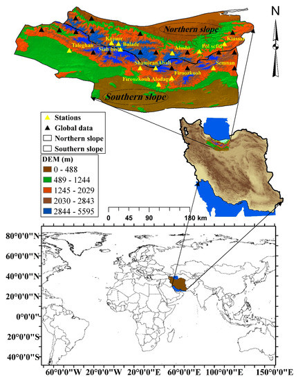
Figure 1.
Study area. The global data in the legend show the data points of the National Centers for Environmental Prediction-Climate Forecast System Reanalysis (NCEP-CFSR).
2.2. Data
2.2.1. Snow Cover Data
To monitor snow cover, MODIS model and Digital Elevation Model (DEM) images were used. To that end, the MOD10A1 and MOD10A2 of MODIS data were first obtained from the NASA National Snow and Ice Data Center (NSIDC) database with a spatial resolution of 500 × 500 m in HDF format. Heavy snowfall in central Alborz usually occurs from early November to May and the snow cover persists until June. For this area, images were available for the 15 years from 2000 to 2014. To process the images, first, a preprocessing operation including geometric, radiometric, and atmospheric corrections was applied to them in ENVI 5.3 software. This operation included calibrating images, converting image coordinates to real terrain coordinates (WGS84 UTM 39N), and removing clouds from images. The following provides a description of the MODIS sensor’s usage applied in the current study to monitor the snow cover area.
One of the five sensors on the Terra satellite is the MODIS sensor, which was launched on December 18, 1999. This sensor’s coverage significantly increased with the launch of the Aqua satellite on May 4, 2002. The MODIS sensor has a spatial resolution (250, 500, and 1000 m), 12-bit radiometric resolution, high temporal resolution (1 to 2 days), and 36-band spectral separation of bands 20 to 23, excluding radiation bands and bands 1 to 7, which are reflective. It covers wavelengths from 0.4 microns (visible light) to 14.4 microns (thermal infrared). The MODIS sensor provides snow cover detection maps using the Normalized Difference Snow Index (NDSI) on a macro-scale and provides a rapid application in regional studies [13]. NDSI is a spectral measure of the relative magnitude of the characteristic reflectance difference between the visible and short-wave infrared reflectance of snow in the MODIS sensor, employed to detect changes in snow cover using the Normalized Difference Vegetation Index (NDVI) algorithm [14]. NDSI uses snow spectral reflectance advantages that exist in the visible band with a high reflectance and infrared spectrum with a low reflectance, and NDSI as an algorithm for detecting snow from clouds and snow-covered areas with a set of thresholds applied and calculated pixel to pixel [14]. In the first method, the dual reflectance criteria (i.e., the pixel reflectance values in band 6 > 11% and the pixel reflectance values in band 4 ≥ 10%) are applied if NDSI > 0.4, based on Equation (1). In the next step, three conditional tests are performed to extract the NDSI values, according to Equation (1). Similar to many spectral rationing methods, this index reduces atmospheric effects [15]. Applying the NDSI will result in the formation of pixels with a value of −1 to +1, for which values ranging from −1 to 0 indicate areas where there is no snow and those from 0 to +1 indicate areas where snow has positive coefficients due to its lightness and heaviness (depending on its depth). When the snow depth is higher, the number is closer to one, and for a lower depth of snow, the number tends toward zero. The MODIS snow map algorithm from bands 4 and 6 of this sensor is automatically implemented to extract the Normalized Difference Snow Index (NDSI) and is calculated based on Equation (1) [16].
In this equation, is the green coverage, which is obtained from band 4 (0.545–0.665 µm) and has a reflectance ≥ 10%. Band 6 (0.841–0.876 µm) has a reflectance > 11% and relates to Short-Wave Infrared (SWIR).
2.2.2. Meteorological Data
In this study, the combined use of the National Centers for Environmental Prediction-Climate Forecast System Reanalysis (NCEP-CFSR) database and observations due to insufficient meteorological stations located at altitude (from the Iranian Meteorological Organization) is provided. The NCEP-CFSR points and the ground stations are specified in Figure 1. The meteorological variables used include the minimum temperature (Tmin), maximum temperature (Tmax), global solar radiation (GSR), relative humidity (RH), precipitation (P), and wind velocity (W), and their units are , , ,, and , respectively. These meteorological data, prepared on monthly scales, belong to the period of 1979–2014 (36 years). These datasets were integrated to be used as inputs for snow cover estimation. As there was one data series for snow cover for each of the northern and southern slopes, the meteorological data had to be integrated into one equivalent series for the estimation and investigation. Therefore, the Thiessen polygon method was used to merge the data into one series, for each of the two slopes of Alborz mountain (according to Guhathakurta et al.’s [17] study). The statistical characteristics of Table 1 refer to the equivalent series.

Table 1.
Statistical characteristics of the monthly data used in this study.
In this investigation, the drought indices were calculated by precipitation and temperature, recorded during the 1979–2014 period. However, according to the limitation of the snow cover data (because of the nonexistence of snow cover images before 2000), investigating the relationship between drought indices and snow cover was conducted for the period of 2000–2014. Furthermore, the estimation of snow cover was implemented for the 2000 to 2014 period. All of the variables, including the snow cover area and meteorological variables, were provided at a monthly scale for all 12 months of the years under study (Table 1 relates to the monthly scale data).
2.3. Drought Indices
Drought indices are used to monitor drought events. Droughts usually begin by precipitation deficit and affect other water resources, appearing as different types, such as meteorological droughts, agricultural droughts, etc. Different types of droughts can be monitored by special individual indices. For example, the Bhalme and Mooley Drought Index (BMDI) is a meteorological drought index and the Palmer Drought Severity Index (PDSI) is an agricultural drought index. On the other hand, there is the Standardized Precipitation Index (SPI), which refers to different types of drought in its different time windows [11]. There are also multivariate drought indices, such as the Joint Deficit Index (JDI) and Multivariate SPI (MSPI), which can monitor different types of drought simultaneously [12,18].
In the current research, seven different drought indices were employed to investigate the effect of drought on snow cover. Table 2 shows the drought indices used. Additionally, references for their calculation methods and supplementary information are provided.
Table 2.
Brief information about the drought indices employed in this study.
2.4. Applied Models
2.4.1. Multiple Linear Regression (MLR)
Multiple linear regression is a linear model implemented between one or more independent variables (input variables) and one dependent variable (target variable). This model is based on the regression coefficients for input variables, which are optimized by the least squares algorithm. In the current research, the inputs were the meteorological variables and the target was the snow cover area. The mathematical form of this model is as follows:
where y is the target (dependent) variable, is the model’s constant coefficient or intercept of the regression line, represents the regression coefficients, represents the input (independent) variables, and is the model’s error.
2.4.2. Least Square Support Vector Machine (LSSVM)
Originating from support vector machines (SVMs), LSSVM is a powerful approach for solving nonlinear classification problems, function estimation, and regression. The SVM, developed by Cortes and Vapnik [26], is based on the principle of construction risk minimization (SRM), which reduces the overestimation of the model [27]. The parameters of this model are γ, representing the adjustment constant, and σ2, representing the radial basis function (RBF) kernel width optimized by the least squares algorithm in this study [6].
2.4.3. Group Method of Data Handling (GMDH)
Ivakhnenko presented GMDH in 1970 at the Ukrainian Institute of Technology. This is a nonlinear multivariate statistical analysis method that can be used to determine the complex structure of input–output relationships in complex systems [28]. GMDH is based on the separation of second- or third-order nested polynomials to simulate regression and classification topics [28]. GMDH is a multilayer network in which each layer is composed of multiple nodes. The results from each layer are transferred to the next layer; in fact, the results of one layer are used as inputs for the next layer [29,30].
2.4.4. Multilayer Perceptron (MLP)
The concept of the perceptron was first introduced by McCulloch and Pitts [31] as an artificial neuron. An MLP network provides a nonlinear relationship between the input and output vectors. This is accomplished by connecting neurons from one layer to another one (previous or next layer). The output of each neuron is multiplied by weight coefficients and given as the input for a nonlinear excitation function [32]. In the training phase, the training data are given to the perceptron, and the grid weights are then adjusted to minimize the error between the target and output of the model, or to reach the default number of training times. Then, like all modeling processes, different inputs (not present in the training phase) are used for model validation. The training of neural networks is generally very complex and can be stated to be an optimization problem with a large number of variables [33].
2.4.5. Multilayer Perceptron-Grey Wolf Optimization (MLP-GWO)
This model results from the integration of the MLP model and the GWO algorithm. The GWO algorithm is a population-based meta-heuristic algorithm that is inspired by the behavior of gray wolves during hunting [34]. This algorithm consists of three main steps: (1) Tracking and approaching; (2) pursing and encircling; and (3) attacking. There are four types of wolf in this algorithm. The alpha wolf is the main driver of the algorithm, the beta and delta wolves act as assistants to the alpha wolf, and the omega wolf follows both the alpha and beta wolves. Gray wolves hunt their prey through surrounding them. At the hunting stage, the gray wolf attacks the surrounded prey. The alpha wolf follows the hunting process, and the beta and delta wolves sometimes participate. For mathematically simulating wolf hunting behavior, it is usually assumed that alpha, beta, and delta wolves have better information on the location of prey [35]. Gray wolves attack and hunt when the target stops moving (see [34] for more information on this optimization algorithm). A schematic diagram of the models used to estimate the snow cover area is shown in Figure 2.
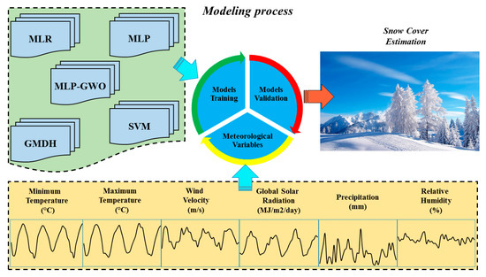
Figure 2.
Schematic diagram of the models’ approaches.
2.5. Model Performance Criteria
Several statistical criteria are used in each study to evaluate the performance of the models. These criteria for current research include the Root Mean Square Error (RMSE), the Normalized Root Mean Square Error (NRMSE), Nash–Sutcliff (NS), and the Willmott Index (WI). The mathematical equations of these indices are as follows:
In these equations, Oi represents the observational data, Ei represents the estimated data, Ō represents the average observational data, Omax represents the maximum observational data, and Omin represents the minimum observational data. The closer values of WI and NS are to 1, and RMSE and NRMSE are to 0, the better the performance of the models.
3. Results
3.1. Investigating the Relationship between Changes in the Snow Cover Area and Drought Indices
The seven drought indices of PDSI, BMDI, SPI, MSPI, SPImod, JDI, and SPEI were initially calculated. Then, the relationship between these indices and the snow cover area for both the northern and southern slopes of the Alborz Mountains was evaluated by the Spearman correlation test. The results of the Spearman test are presented in Table 3 and Table 4.
Table 3.
Spearmen correlation test results on the relationship between the indexes and snow cover for the northern slope.
Table 4.
Spearmen correlation test results on the relationship between the indexes and snow cover for the southern slope.
Here, 24 time windows of the indices SPI, SPEI, and SPImod were calculated for each slope. The results indicate a significant relationship (p = 0.01) between the snow cover area and SPI for both the northern and southern slopes of Alborz and some SPEI time windows for the southern slope. The highest correlation coefficients were observed in SPI 1-, 2-, 3-, 4-, 5-, and 6-month time windows and accordingly, MSPI was calculated in time windows of 1–3 months (MSPI1–3), 1–6 months (MSPI1–6), 1–9 months (MSPI1–9), and 1–12 months (MSPI1–12). The five main time windows mentioned in the introduction of MSPI [23] were also calculated and investigated (including MSPI3–6, MSPI6–12, MSPI3–12, MSPI12–24, and MSPI24–48). The drought indices, including SPImod (in all time windows), MSPI (in all time windows), JDI, BMDI, and PDSI, were not significantly related to snow cover variations. The highest correlation coefficients for the northern slope were 0.723 and 0.720, which were reported for SPI2 and SPI3, respectively. For the southern slope, the highest correlation coefficients were 0.617 and 0.638, which respectively belong to SPI1 and SPI2. The most important reasons for this are the higher humidity and cloudiness and consequently lower evaporation rates of the northern slopes, and conversely, the higher received radiation rates for the southern slopes. This causes the snow to melt later on the northern slopes. Therefore, the effects of snow cover on droughts will remain longer and consequently, larger time windows of SPI can be related to the snow cover area for the northern slopes. As a result, SPI2 can be identified as the best time window of SPI and the drought variable (among these indices) most related to the snow cover variations in this region. In general, it can be reported that the drought status will be most effective during the increasing and decreasing of the snow cover area with a two-month time lag, remaining for up to five (or six) months.
3.2. Results of Snow Cover Estimation
3.2.1. Input Selection
Prior to modeling, the correlation matrix was used at the input selection stage. The correlation results of the variables are shown in Figure 3.
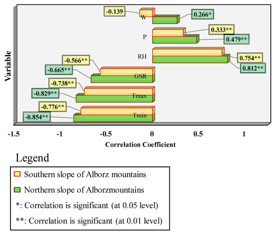
Figure 3.
Correlation between the meteorological data and snow cover for the northern and southern slopes of Alborz Mountains.
There is a rational and strong negative correlation between the maximum and minimum temperatures, as well as between radiation and snow cover areas, for both slopes. Moreover, in terms of the positive correlations, the relative humidity has a strong correlation with the snow cover and precipitation has a weaker positive correlation coefficient, but both of them are significant at the 0.01 level. The variable wind speed had the weakest correlation for both slopes, being significant at the 0.05 level for the northern slope and insignificant for the southern slope. The opposite direction of the wind speed’s correlation for these two slopes can be related to the influential synoptic systems. The northern slope of Alborz Mountains is affected by the fronts from the Mediterranean Sea, Black Sea, and Caspian Sea. The absolute majority of rainfall due to these systems falls at the northern slope and a much smaller amount falls in the southern zones, which causes a big difference between these two areas’ climates (north of these mountains, there are humid and super-humid climates and, to the south, there is an arid climate). The wind speed close to the earth’s surface, especially at altitude and in mountainous regions, is significantly related to the atmospheric fronts’ speed. Therefore, when the wind speed increases, a front transfers the moisture to altitude and causes snowfall, so the snow cover area will increase. However, the front loses its humidity and after descending the altitudes in the southern part, it usually produces chinook wind. This phenomenon causes snowmelt and decreases the snow cover area, so there will be a negative relation between snow cover and wind speed in this region.
In these datasets, the precipitation refers to rainfall data. Also at high altitudes, the snowfall events are transformed into water equivalents of snow and count as rainfall. It is obvious that snowfall can increase the snow cover and causes a positive correlation with the snow cover area. In contrast, warm precipitation causes a negative correlation. As we can see for the correlations, there are positive correlations (+0.333 for the southern slope and +0.479 for the northern slope) between the snow cover area and precipitation. To extend this issue, it can be stated that, at lower altitudes, warmer seasons have warm precipitation, which melts the snow and causes a negative correlation with the snow cover area, and colder seasons have both cold and warm precipitation. However, almost all of the precipitation at high altitudes occurs in the form of snowfall, which increases the snowy area and has a positive correlation with the snow cover area. Since the snow cover area exists at higher altitudes, cold precipitation and snowfall will be more effective in terms of the snow cover. Therefore, in the general form of this region, precipitation will be positively correlated with the snow cover area.
The correlation of snow cover with meteorological variables is somewhat stronger for the northern slope, because the standard deviation, skewness, and coefficient of variation of this phenomenon (snow cover area) are lower for the northern slope, so it is somewhat closer to exhibiting a normal distribution. This phenomenon can lead to less variability and, consequently, greater consistency with other meteorological variables. To select the inputs, the meteorological variables for each slope were sorted separately by the correlation coefficients, and the input scenarios were selected as given in Table 5.
Table 5.
Input scenarios of the models for each slope.
Therefore, input scenarios, inputs (meteorological variables), and the target (snow cover area) were arranged, and in each scenario, 75% of the number of months was selected for training and 25% for the test. Then, five methods, including MLR, LSSVM, GMDH, MLP, and MLP-GWO, were used for estimating the snow cover.
3.2.2. Models’ Performances
This section only covers the test part, and the results are listed in Table 6. It can be observed that the MLR model is the weakest model in most cases.
Table 6.
Results of snow cover estimation by the models.
This indicates that the nonlinear relationships between the meteorological variables and the snow cover area are stronger than the linear relationships. The best performance in the northern and southern slopes belongs to the MLR6 and MLR3 scenarios, respectively. The equations derived from MLR models are given below:
These equations are applicable for these two slopes for estimating the snow cover if no snow cover data are available. Equation (8) is the best MLR model for southern slopes, as it has the least error and can also be used with just three variables, including , , and .
Subsequently, the SVM and MLP artificial intelligence models performed relatively well in terms of the accuracy. Both of these models displayed their best performance with scenario 6 and the model performance can be considered very desirable, with NS > 0.75 and NRMSE < 0.10. However, the NRMSE value for these two models is more than 0.10 for the southern slope.
Among the AI-based models, the GMDH and/or MLP-GWO models produced the best results in all scenarios. GMDH provided its best estimation with the fourth input scenario (GMDH4), exhibiting results of RMSE = 816.011 km2, NRMSE = 0.089, NS = 0.918, and WI = 0.979 for the northern slope, and with the sixth input scenario (GMDH6), displaying results of RMSE = 1111.549 km2, NRMSE = 0.087, NS = 0.877, and WI = 0.965, for the southern slope. The most accurate performance of MLP-GWO for the northern slope resulted from the MLP-GWO6 input scenario, with RMSE = 754.711 km2, NRMSE = 0.083, NS = 0.930, and WI = 0.980. For the southern slope, the MLP-GWO2 input scenario produced the best estimation, with RMSE = 1261.877 km2, NRMSE = 0.098, NS = 0.842, and WI = 0.953. The NRMSE < 0.10 and NS > 0.80 for the southern slope and NS > 0.90 for the northern slope show that the performances of GMDH and MLP-GWO can be highly desirable and superior to the other models in the estimation of snow cover.
The GMDH model, with many optimization parameters, such as the number of layers and the number of each layer’s neurons, can provide several make ups to adjust its network structure, whereas the LSSVM model only uses two parameters for optimization (Table 6). The MLP model is similar to the GMDH in terms of having several optimization parameters. However, it uses the GWO algorithm, which can increase the accuracy of MLP (with an average of 10.7% improvement) by selecting the optimal parameters. The optimal parameters of the machine learning approaches are provided in Table 7.
Table 7.
Parameters of the machine learning models.
Correlation graphs were used to compare the correlation between the snow cover estimation and the actual values (Figure 4 and Figure 5). Here, the weakest coefficient of determination (for both slopes) is also reported in MLR estimation. For the northern slope (Figure 4), the highest R2 is observed in the GMDH outputs (R2 = 0.92 in GMDH4 and GMDH5), and then in the MLP-GWO model estimation (where R2 reaches 0.91 in MLP-GWO3 and MLP-GWO4). The mean coefficients of determination are lower for the southern slope (Figure 5). The weakest coefficient of determination belongs to MLR1 and MLR2, with R2 = 0.68. The strongest result of this slope belongs to GMDH6, with R2 = 0.88. These values indicate the favorable estimates of the snow cover provided by the GMDH and MLP-GWO models.
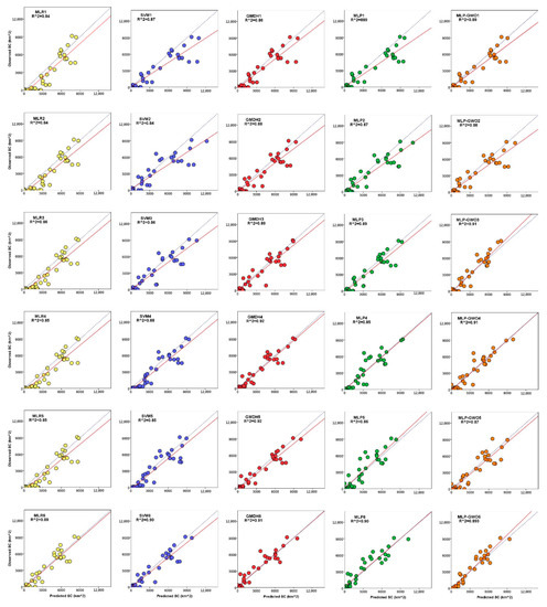
Figure 4.
Regression plots of the models’ outputs for the northern slope (SC = snow cover).
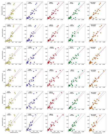
Figure 5.
Regression plots of the models’ outputs for the southern slope (SC = snow cover).
Taylor diagrams were plotted for the models’ outputs, as shown in Figure 6 and Figure 7. As there are a large number of models, only two Taylor diagrams were plotted for each slope: The first diagram displays the MLR, SVM, and GMDH outputs, and the second diagram displays the MLP and MLP-GWO outputs. The weakest estimates (points farthest from Obs) are points G and H, which belong to LSSVM1 and LSSVM2, respectively, for the northern slope (Figure 6). The most accurate estimates are the points P, Q, u, and x, which were obtained for GMDH4, GMDH5, MLP-GWO3, and MLP-GWO6, respectively. These points are located closest to the Obs point between the two dashed lines of RMSE = 1000 km2 and RMSE = 500 km2 and below the R = 0.95 line. For the southern slope (Figure 7), the weakest estimates were obtained for points A and B, which belong to MLR1 and MLR2, and they are close to the R = 0.80 line. The most accurate estimation for this slope is the R point of GMDH6. This point is the closest mode to the R = 0.95 line and RMSE = 1000 km2 dashed line. The effect of using the GWO algorithm on MLP optimization can be observed for both slopes, where, in all cases (with similar inputs), the MLP-GWO points are in a better position than the MLP points, indicating the relatively better performance of this model in estimating snow cover areas.
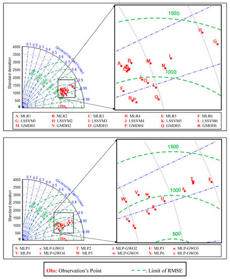
Figure 6.
Taylor diagram of the models’ outputs for the northern slope.
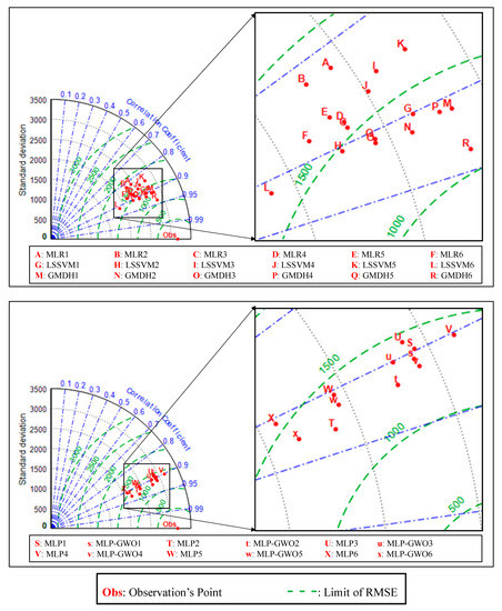
Figure 7.
Taylor diagram of the models’ outputs for the southern slope.
In another graphical form, the frequency distribution of the observed and estimated snow cover data was plotted by a violin plot (Figure 8). Here, the frequency distribution of the most accurate performances of each model is examined in the form of violins [36]. The similarity of the violins to the actual snow cover data violins may indicate that the frequency distribution of the estimated data is close to the actual data. For the northern slope, the GMDH outputs, followed by the MLP-GWO outputs, have the most curvature similar to the observational data violin (particularly GMDH, which performed very desirably in showing data curvature greater than the third quartile). The violin of the southern slope observational data is more complex. This complexity is due to the presence of two months of snow cover at the upper tail end of the distribution. Among the models, the GMDH model was able to estimate one of these two exceptional months, which is beyond the capability of the other four models, particularly MLR and LSSVM. In estimating the violin curvature of the observational data, GMDH generally has the closest possible curvature to the observational data.
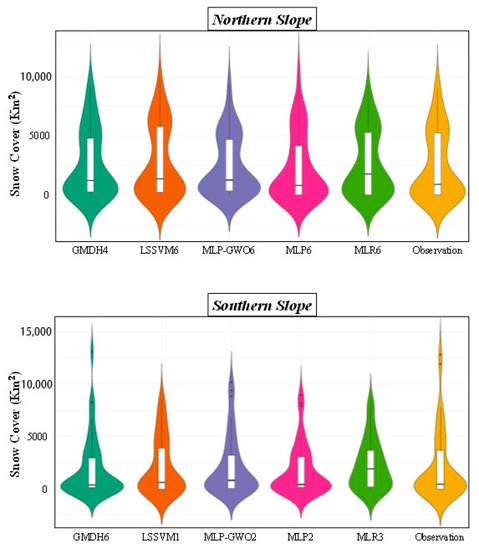
Figure 8.
Violin plots for comparing the distributions of outputs and observations.
4. Discussion
Due to the lack of studies on snow cover area estimation, we can follow studies on the estimation of other snow variables [9], as discussed. Estimates of snow depth in the German Black Forest mountains were obtained using inputs similar to this study (except for the fact that the average temperature was used instead of the maximum and minimum temperatures) [37]. In the study, the MODIS sensor was used to monitor the snow depth and the estimator models were similar to the artificial intelligence-based models. The results of this study with 0.83 < R < 0.93, like the current study, indicated the accuracy of artificial intelligence models for estimating the desired snow variables. The MLP model with precipitation, minimum, and maximum temperature inputs was used to estimate the maximum daily fresh snow accumulation (MDFSA) in South Korea [9]. This model presented a desirable result, with a correlation coefficient of R = 0.90, which is consistent with the results of the present study. Binaghi et al. [38] used the RBF neural network to estimate the thickness (depth) of snow in the central Alpine area in Italy. Meteorological inputs (temperature and precipitation) were used in the study and NRMSE ranged from 0.04 to 0.07, indicating a better accuracy than the current study. This difference may be due to the nature of the variable (snow depth) itself, which can be explained by the fact that its estimation (based on the normalized RMSE) is more accurate than estimating the snow cover area.
5. Conclusions
This study investigated the relationships between several drought indexes, including PDSI, BMDI, SPI, MSPI, SPImod, JDI, and SPEI, and the snow cover area, and compared the accuracies of the artificial intelligence-based models, MLR, LSSVM, GMDH, MLP, MLP-GWO, and MLR in estimating the snow cover area using meteorological inputs, precipitation, the minimum and maximum temperature, the global solar radiation, the relative humidity, and the wind velocity. The evaluation of the correlations between drought indices and the snow cover area showed that the effect of drought on snow cover would remain up to 5 (or 6) months in the region. The most related index is the time window 2 of SPI (SPI2), which shows that the effectiveness of a drought event will appear after two months based on snow cover variations. The outcomes of this study obtained in the modeling part confirmed that MLP-GWO and GMDH models can be considered acceptable for estimating the snow cover area of a region. The application of these data-driven models is significant in the following cases: (1) Difficulty in field measurements of the snow cover area; (2) a lack of accessibility to satellite images for monitoring the snow cover area; (3) estimation of the snow cover area in missing months; and (4) estimation of the snow cover area in years without satellite images. This study was conducted on a monthly scale, but a limitation for snow studies, at a daily scale, is the separation of snow from cloud. It can cause errors in monitoring the snow cover area and produces missing daily data. For this subject, the 8–day images of MODIS, or images of the other sensors such as Landsat, SPOT, ASTER, etc., can be used. The results of this study in both sections are acceptable and promising, and are well worth researching elsewhere in the world. They suggest using and testing other types of drought indices to further investigate snow cover variations’ effects on droughts. Furthermore, other artificial intelligence-based models, such as ANFIS, RBF, and GRNN, and different optimization algorithms, such as the Genetic Algorithm, Particle Swarm Optimization, Firefly Algorithm, etc., are suggested for snow cover estimation.
Author Contributions
Research Idea, P.A.; Conceptualization, P.A. and B.M.; methodology, P.A., H.B.-P. and B.M.; software, P.A., H.B.-P. and B.M.; validation, P.A. and B.M.; investigation, P.A. and B.M.; data curation, P.A. and H.B.-P.; writing–original draft preparation, P.A., H.B.-P. and B.M.; writing–review and editing, Y.G., O.K., and, D.Z.; supervision, Y.G., O.K., and D.Z. All authors have read and agreed to the published version of the manuscript.
Funding
This research received no external funding.
Conflicts of Interest
The authors declare no conflict of interest.
References
- Tsai, Y.L.S.; Dietz, A.; Oppelt, N.; Kuenzer, C. Remote sensing of snow cover using spaceborne SAR: A review. Remote Sens. 2019, 11, 1456. [Google Scholar] [CrossRef]
- Broxton, P.D.; Harpold, A.A.; Biederman, J.A.; Troch, P.A.; Molotch, N.P.; Brooks, P.D. Quantifying the effects of vegetation structure on snow accumulation and ablation in mixed-conifer forests. Ecohydrology 2015, 8. [Google Scholar] [CrossRef]
- Stone, R.S.; Dutton, E.G.; Harris, J.M.; Longenecker, D. Earlier spring snowmelt in northern Alaska as an indicator of climate change. J. Geophys. Res. Atmos. 2002, 107. [Google Scholar] [CrossRef]
- Adam, J.C.; Hamlet, A.F.; Lettenmaier, D.P. Implications of global climate change for snowmelt hydrology in the twenty-first century. Hydrol. Process. 2009, 23, 962–972. [Google Scholar] [CrossRef]
- Lindsay, C.; Zhu, J.; Miller, A.E.; Kirchner, P.; Wilson, T.L. Deriving snow cover metrics for Alaska from MODIS. Remote Sens. 2015, 7, 12961–12985. [Google Scholar] [CrossRef]
- Liu, C.; Huang, X.; Li, X.; Liang, T. MODIS fractional snow cover mapping using machine learning technology in a mountainous area. Remote Sens. 2020, 12, 962. [Google Scholar] [CrossRef]
- Mohammadi, B.; Mehdizadeh, S. Modeling daily reference evapotranspiration via a novel approach based on support vector regression coupled with whale optimization algorithm. Agric. Water Manag. 2020, 237. [Google Scholar] [CrossRef]
- Roebber, P.J.; Bruening, S.L.; Schultz, D.M.; Cortinas, J.V. Improving snowfall forecasting by diagnosing snow density. Weather Forecast. 2003, 18. [Google Scholar] [CrossRef]
- Tabari, H.; Marofi, S.; Abyaneh, H.Z.; Sharifi, M.R. Comparison of artificial neural network and combined models in estimating spatial distribution of snow depth and snow water equivalent in Samsami basin of Iran. Neural Comput. Appl. 2010, 19. [Google Scholar] [CrossRef]
- Lee, G.; Kim, D.; Kwon, H.H.; Choi, E. Estimation of maximum daily fresh snow accumulation using an artificial neural network model. Adv. Meteorol. 2019, 2019. [Google Scholar] [CrossRef]
- Khadka, D.; Babel, M.S.; Shrestha, S.; Tripathi, N.K. Climate change impact on glacier and snow melt and runoff in Tamakoshi basin in the Hindu Kush Himalayan (HKH) region. J. Hydrol. 2014, 511. [Google Scholar] [CrossRef]
- Aghelpour, P.; Bahrami-Pichaghchi, H.; Kisi, O. Comparison of three different bio-inspired algorithms to improve ability of neuro fuzzy approach in prediction of agricultural drought, based on three different indexes. Comput. Electron. Agric. 2020, 170. [Google Scholar] [CrossRef]
- Salomonson, V.V.; Appel, I. Estimating fractional snow cover from MODIS using the normalized difference snow index. Remote Sens. Environ. 2004, 89. [Google Scholar] [CrossRef]
- Klein, A.G.; Hall, D.K.; Riggs, G.A. Improving the MODIS global snow-mapping algorithm. In Proceedings of the International Geoscience and Remote Sensing Symposium (IGARSS), Singapore, 3–8 August 1997; Volume 2. [Google Scholar]
- Hall, D.K.; Riggs, G.A.; Salomonson, V.V.; DiGirolamo, N.E.; Bayr, K.J. MODIS snow-cover products. Remote Sens. Environ. 2002, 83. [Google Scholar] [CrossRef]
- Bashir, F.; Rasul, G. Estimation of average snow cover over northern pakistan. Pakistan J. Meteorol. 2008, 7. [Google Scholar]
- Guhathakurta, P.; Sreejith, O.P.; Menon, P.A. Impact of climate change on extreme rainfall events and flood risk in India. J. Earth Syst. Sci. 2011, 120. [Google Scholar] [CrossRef]
- Bazrafshan, J.; Nadi, M.; Ghorbani, K. Comparison of Empirical Copula-Based Joint Deficit Index (JDI) and Multivariate Standardized Precipitation Index (MSPI) for Drought Monitoring in Iran. Water Resour. Manag. 2015, 29. [Google Scholar] [CrossRef]
- Palmer, W.C. Meteorological Drought; No. 45; US Department of Commerce, Weather Bureau: Washington, DC, USA, 1965. [Google Scholar]
- Van Der Schrier, G.; Jones, P.D.; Briffa, K.R. The sensitivity of the PDSI to the Thornthwaite and Penman-Monteith parameterizations for potential evapotranspiration. J. Geophys. Res. Atmos. 2011, 116. [Google Scholar] [CrossRef]
- Bhalme, H.N.; Mooley, D.A. Large-scale droughts/ floods and monsoon circulation. Mon. Weather Rev. 1980, 108. [Google Scholar] [CrossRef]
- McKee, T.B.; Nolan, J.; Kleist, J. The relationship of drought frequency and duration to time scales. In Proceedings of the Eighth Conference on Applied Climatology, Anaheim, CA, USA, 17–22 January 1993. [Google Scholar]
- Bazrafshan, J.; Hejabi, S.; Rahimi, J. Drought monitoring using the multivariate standardized precipitation index (MSPI). Water Resour. Manag. 2014, 28. [Google Scholar] [CrossRef]
- Kao, S.C.; Govindaraju, R.S. A copula-based joint deficit index for droughts. J. Hydrol. 2010, 380. [Google Scholar] [CrossRef]
- Vicente-Serrano, S.M.; Beguería, S.; López-Moreno, J.I. A multiscalar drought index sensitive to global warming: The standardized precipitation evapotranspiration index. J. Clim. 2010, 23. [Google Scholar] [CrossRef]
- Cortes, C.; Vapnik, V. Support-Vector Networks. Mach. Learn. 1995, 20. [Google Scholar] [CrossRef]
- Moazenzadeh, R.; Mohammadi, B.; Shamshirband, S.; Chau, K. Coupling a firefly algorithm with support vector regression to predict evaporation in northern Iran. Eng. Appl. Comput. Fluid Mech. 2018, 12, 584–597. [Google Scholar] [CrossRef]
- Ivakhnenko, A.G. Heuristic self-organization in problems of engineering cybernetics. Automatica 1970, 6. [Google Scholar] [CrossRef]
- Aghelpour, P.; Varshavian, V. Evaluation of stochastic and artificial intelligence models in modeling and predicting of river daily flow time series. Stoch. Environ. Res. Risk Assess. 2020, 34, 33–50. [Google Scholar] [CrossRef]
- Ashrafzadeh, A.; Kişi, O.; Aghelpour, P.; Biazar, S.M.; Masouleh, M.A. Comparative study of time series models, support vector machines, and gmdh in forecasting long-term evapotranspiration rates in northern iran. J. Irrig. Drain. Eng. 2020, 146. [Google Scholar] [CrossRef]
- McCulloch, W.S.; Pitts, W. A logical calculus of the ideas immanent in nervous activity. Bull. Math. Biophys. 1943, 5. [Google Scholar] [CrossRef]
- Mohammadi, B.; Ahmadi, F.; Mehdizadeh, S.; Guan, Y.; Pham, Q.B.; Linh, N.T.T.; Tri, D.Q. Developing novel robust models to improve the accuracy of daily streamflow modeling. Water Resour. Manag. 2020. [Google Scholar] [CrossRef]
- Vaheddoost, B.; Guan, Y.; Mohammadi, B. Application of hybrid ANN-whale optimization model in evaluation of the field capacity and the permanent wilting point of the soils. Environ. Sci. Pollut. Res. 2020. [Google Scholar] [CrossRef]
- Mirjalili, S.; Mirjalili, S.M.; Lewis, A. Grey wolf optimizer. Adv. Eng. Softw. 2014, 69. [Google Scholar] [CrossRef]
- Muro, C.; Escobedo, R.; Spector, L.; Coppinger, R.P. Wolf-pack (Canis lupus) hunting strategies emerge from simple rules in computational simulations. Behav. Processes 2011, 88. [Google Scholar] [CrossRef] [PubMed]
- Aghelpour, P.; Mohammadi, B.; Biazar, S.M. Long-term monthly average temperature forecasting in some climate types of Iran, using the models SARIMA, SVR, and SVR-FA. Theor. Appl. Climatol. 2019, 138, 1471–1480. [Google Scholar] [CrossRef]
- Sauter, T.; Weitzenkamp, B.; Schneider, C. Spatio-temporal prediction of snow cover in the Black Forest mountain range using remote sensing and a recurrent neural network. Int. J. Climatol. 2010, 30. [Google Scholar] [CrossRef]
- Binaghi, E.; Pedoia, V.; Guidali, A.; Guglielmin, M. Snow cover thickness estimation using radial basis function networks. Cryosphere 2013, 7. [Google Scholar] [CrossRef]
Publisher’s Note: MDPI stays neutral with regard to jurisdictional claims in published maps and institutional affiliations. |
© 2020 by the authors. Licensee MDPI, Basel, Switzerland. This article is an open access article distributed under the terms and conditions of the Creative Commons Attribution (CC BY) license (http://creativecommons.org/licenses/by/4.0/).