Article

Hierarchical Multi-Label Object Detection Framework for Remote Sensing Images

Agency for Defense Development, Institute of Defense Advanced Technology Research, Daejeon 34186, Korea
*
Author to whom correspondence should be addressed.
Remote Sens. 2020, 12(17), 2734; https://doi.org/10.3390/rs12172734
Submission received: 16 July 2020 / Revised: 14 August 2020 / Accepted: 21 August 2020 / Published: 24 August 2020

Abstract

:
Detecting objects such as aircraft and ships is a fundamental research area in remote sensing analytics. Owing to the prosperity and development of CNNs, many previous methodologies have been proposed for object detection within remote sensing images. Despite the advance, using the object detection datasets with a more complex structure, i.e., datasets with hierarchically multi-labeled objects, is limited to the existing detection models. Especially in remote sensing images, since objects are obtained from bird’s-eye view, the objects are captured with restricted visual features and not always guaranteed to be labeled up to fine categories. We propose a hierarchical multi-label object detection framework applicable to hierarchically partial-annotated datasets. In the framework, an object detection pipeline called Decoupled Hierarchical Classification Refinement (DHCR) fuses the results of two networks: (1) an object detection network with multiple classifiers, and (2) a hierarchical sibling classification network for supporting hierarchical multi-label classification. Our framework additionally introduces a region proposal method for efficient detection on vain areas of the remote sensing images, called clustering-guided cropping strategy. Thorough experiments validate the effectiveness of our framework on our own object detection datasets constructed with remote sensing images from WorldView-3 and SkySat satellites. Under our proposed framework, DHCR-based detections significantly improve the performance of respective baseline models and we achieve state-of-the-art results on the datasets.

Graphical Abstract

1. Introduction

Driven by the improved accessibility to remote sensing images, many deep convolutional neural network (CNN)-based object detection approaches have gained more attention recently. The successes of the deep detectors on remote sensing images facilitate a wide range of civil and military applications, such as urban planning [1], surveillance [2], crop monitoring [3], traffic planning [4], vehicle tracking [5], building detection [6,7], and military uses [8]. For the research purposes, several remote sensing object detection datasets such as DOTA [9], HRSC2016 [10], and NWPU VHR-10 [11] have been released and used in numerous works. Object detection with such public remote sensing datasets gives rise to following challenges: (1) since remote sensing images are obtained from bird’s-eye view, the restricted visual features of objects are captured; (2) objects appear with large scales variability in remote sensing images; and (3) the geospatial distributions of objects are highly imbalanced across multiple images as well as across different categories.
However, the public remote sensing object detection datasets are gathered from limited regions with some pre-defined categories, which restricts the flexible research usage in part. We construct our own datasets with 963 WorldView-3 images and 457 SkySat images covering harbor and airport peripheral areas, provided by DigitalGlobe [12] and Planet Labs [13] respectively. In our datasets, various types of aircraft and ship objects are labeled by experts in aerial image interpretation. Prior to directly exploiting the raw remote sensing images as the object detection datasets, it is worth noting the following conditions. First, the raw remote sensing images are very large in size (e.g., typically larger than 5000 × 5000 pixels). In public datasets, the raw aerial images were preprocessed into relatively small chips in general, so that it can be conveniently used for both training and testing. Secondly, the objects in our datasets are labeled in varying degrees depending on the amount of visual information and the resolutions of images, which leads to hierarchically partial annotations. Figure 1 shows some examples that one aircraft is labeled “aircraft (coarse1)|civilian-aircraft (coarse2)”, while the other aircraft are more elaborately annotated as “aircraft (coarse1)|civilian-aircraft (coarse2)|B-747 (fine)” or “aircraft (coarse1)|civilian-aircraft (coarse2)|A-380 (fine)”.
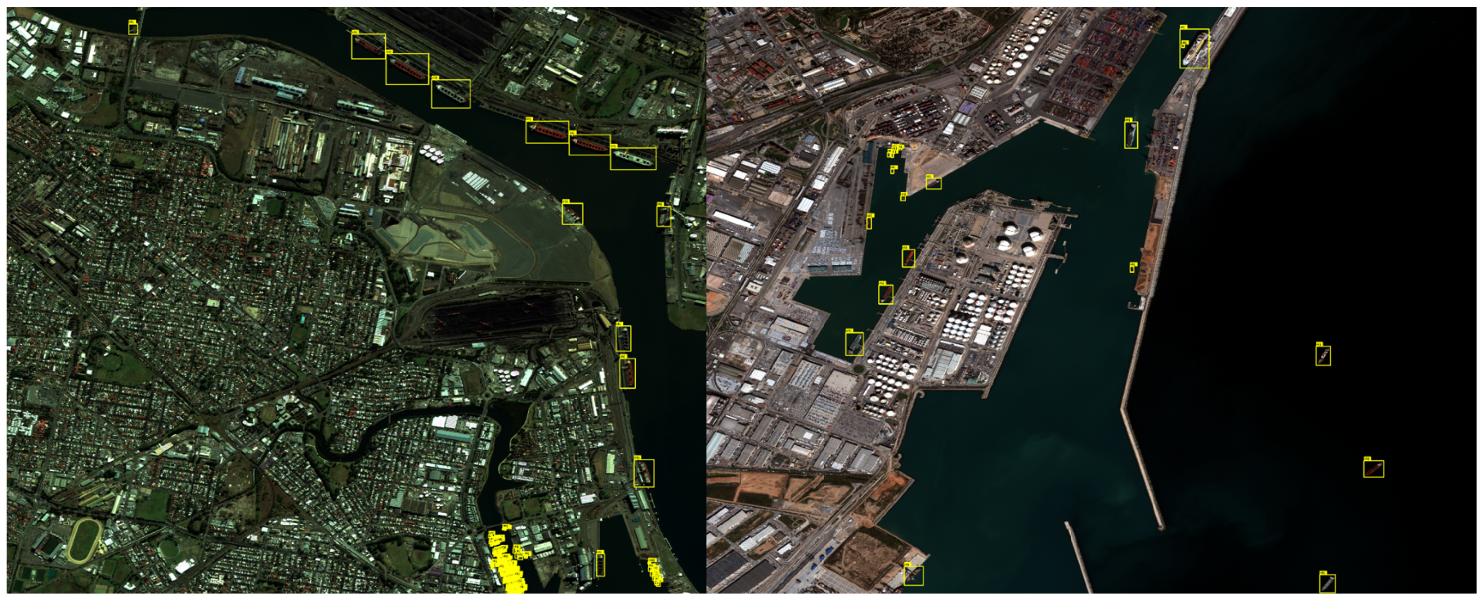
Due to the aforementioned first issue, given a huge remote sensing image we must explore the whole pixels during inference, suffering from high computational costs. In order to compensate the inefficient exploring process, we need an intensive region proposal strategy before performing the object detection. If ships are target objects, sea areas or shorelines would be of great importance in the ship detection rather than fully inland areas. Figure 2 provides two examples of actual remote sensing images taken from harbor-peripheral areas, where the ship objects are sparsely distributed in the aerial images. Inspired by this motivation, some researchers have been presented the region proposal methods for selectively analyzing regions on vast areas [14,15]. CRPN [14] generates the cropping regions by uniting boundaries of inferred object proposals, and CPNet [16] infers the candidate region proposals, trained with cluster groundtruth annotations generated by mean-shift algorithm [15]. We propose a novel region cropping strategy partially inspired by CRPN and CPNet. We also infer object proposals similarly to CRPN and after that, we perform the mean-shift clustering algorithm on the inferred object proposals. Unlike CPNet, we are not required to generate cluster groundtruth annotations. Also, we do not need to set any hyper-parameter because the mean-shift algorithm automatically finds the appropriate number of clusters fitted with data instances; meanwhile, CRPN sets a scale threshold for the generation of cropping regions.
On the other hand, handling the hierarchically partial-annotated objects mentioned as the second issue needs help basically from hierarchy-based detection methods. However, as majority of previous studies have been developed with the benchmark object detection datasets, where the objects are annotated with pre-defined fine labels arranged in a “flat” structure. Little research considers such datasets with hierarchically partial-annotated objects in object detection. Although it does not exactly match our dataset setting, there have been several works dealing with CNN-based hierarchical classification on natural images [17,18]. HD-CNN [17] learns classification components on coarse and subset of fine labels at the two levels and outputs a final probability distribution over fine labels. Ouyang et al. in [18] finetunes deep models, where a deep model for a group of classes is initialized with its parent deep model. Sharing the similar spirit as works [17,18], we devise a Hierarchical Sibling Classification Network (HSCN) by separately deploying classification modules on each set of sibling classes at all levels. We exploit the classification modules that are simple yet fully dense, instead of deep models as in [18]. Our approach leads to an end-to-end learning without the consecutively finetuning processes. Additionally, we minimize unnecessary competitions of a SoftMax function across all classes by replacing the SoftMax function with multiple SoftMax functions over sets of sibling classes when training HSCN, which differentiates our modeling from the approach of [17].
In this paper, we propose a hierarchical multi-label object detection framework for remote sensing images with the hierarchically partial-annotated datasets. This framework takes a raw remote sensing image of an arbitrary size as input, extracts interesting regions of the image, and then performs hierarchical multi-label object detection on the regions. The proposed framework consists of two parts.
The first part is a clustering-guided cropping strategy, which quickly infers candidate object proposals and generates region crops tightening the clustered object proposals. Because we cannot speculate the exact position of objects before detection inference, the existing approach attempted to divide the whole aerial scene into sub-patch images and run inference over the all patch images. Our proposed clustering-guided cropping strategy tackles the inefficient detection process and resolves the problem through the shrinkage of exploration space via expedite objectness inference and clustering. Clustering on the roughly inferred objects leads to generating cluster crops which are valuable regions among whole scene areas to be intensively inferred. In the case that the time of decision making is a critical factor, our clustering-guided cropping strategy would play an important role in improving inference speed without sacrificing significant performance.
The second part is a novel hierarchical multi-label object detection pipeline called Decoupled Hierarchical Classification Refinement (DHCR), which involves two networks; one is a detection network with multiple classifiers and the other is a classification network called HSCN for hierarchical multi-labeling. The key common modelings for the two networks are locally deployment of classifiers for adapting to our hierarchically partial-annotated datasets. We are specifically inspired by the work of decoupled classification refinement (DCR) [19], which jointly accompanies a detection network and a classification network. The advantages of our proposed object detection pipeline called DHCR are: (1) DHCR can handle hierarchically partial-annotated dataset through the separation of classifiers, (2) DHCR can classify objects hierarchically through hierarchical classification results, and (3) DHCR can expect the improvement of classification accuracy at fine level as in DCR.
We carry out experiments on our own object detection datasets acquired from WorldView-3, SkySat satellites. For verifying the validity of the proposed framework, we qualitatively analyze by visualizing the experimental results, and quantitatively evaluate the performance with several rotational-box-based detector baselines. DHCR-based detections significantly boost the performance of the respective baseline models and we achieve state-of-the-art results on our own datasets.
In summary, our contributions are four-fold:
  • We are the first to tackle the hierarchical multi-label object detection problem under the hierarchically partial-annotated dataset settings.
  • We propose a clustering-guided cropping strategy which infers object proposals via a deep detector and followed by clustering the object proposals by a clustering algorithm, which supports more efficient testing in subsequent object detection.
  • We introduce a hierarchical multi-label object detection pipeline, DHCR, that are composed of a detection network with multiple classifiers and a classification network for hierarchical multi-labeling to train on arbitrarily hierarchical-annotated datasets and improve the performance of object detection.
  • The extensive qualitative and quantitative experiments on our own datasets with WorldView-3 and SkySat satellite images suggest that the proposed object detection framework is a practical solution for cropping regions and detecting objects with hierarchical multi-labels.
The rest of this paper is organized as follows. Section 2 reviews related works on (1) object detection and applications of CNN in remote sensing images, (2) region proposal methods for aerial images, and (3) CNN-based hierarchical multi-label classification. The detailed design of our proposed object detection framework is described in Section 3. Section 4 reports comparative experimental results for the proposed object detection framework on our own datasets. Finally, Section 6 includes the final remarks and a conclusion.

2. Previous Work

We first introduce object detection and applications of CNN in remote sensing images. Then we review two lines of works that are the most relevant to ours; region proposal methods for aerial images, and CNN-based hierarchical multi-label classification.

2.1. Object Detection and Applications of CNN in Remote Sensing Images

Due to rapid deep learning breakthroughs, CNN-based detection models have also drawn interest in the field of object detection on remote sensing images. In order to detect and count cars in unmanned aerial vehicle images, Ammour et al. [20] extracted features of regions through pre-trained CNNs and classify whether the regions are car via a linear support vector machine [21]. Another recent studies for vehicle detection are: Audebert et al. [22] proposed a deep-learning-based segment-before-detect method for segmentation followed by detection and classification, and Zhong et al. [5] combined two networks; one network generates a set of vehicle-like regions, and the other network takes a cascaded hierarchical feature learning approach. As military and civilian infrastructures, airports have been also studied for object detection [23,24]. For detecting ships with different scales and large appearance variation, the previous works [2,25] developed variants of Feature Pyramid Network [26], where Yang et al. built high-level semantic feature-maps for all scales [25], and Fu et al. [2] used deep reinforcement learning to get accurate ship angle information. As another application, Chen et al. [27] aimed at end-to-end airplane detection with a single deep CNN based on transfer learning. A few works have been proposed to detect fir trees for the forest health assessment in a quicker and cheaper way [3], and detect oil palm trees for predicting the yield of palm oil, monitoring the process of growth and resulting in the maximum productivity [28].

2.2. Region Proposal Methods for Aerial Images

The aerial images generally cover vain areas and such characteristic has been motivated many researchers to develop region proposal methods for focusing on regions selectively. The purposes of previous works on the region proposal methods can be viewed from two aspects. First, object detection needs to be conducted on certain areas excluding the massive backgrounds with very little chance of target objects being present [14,29]. Secondly, because objects taken in the aerial images are very small in pixels and distributed sparsely and non-uniformly, e.g., pedestrians or vehicles, object detectors can show improvement by re-executing object detection especially in zoom-out images whose target objects are densely crowded [16,30].
For the former purpose, the work in [14] proposed a Cropping Region Proposal Network (CRPN), which exploits a weak semantic RPN quickly searching for candidate object proposals and unites neighboring objects based on Intersection-over-Union (IoU). The other work sharing the same purpose [29] predicted whether objects exist or not for a patch image generated by a sliding-window fashion. Given in a patch image, Pang et al. [29] extracted a feature vector on the patch image via a lightweight residual network called Tiny-Net and a classifier takes the feature vector for the binary objectness prediction. For the latter purpose, a Density Map guided-detection Network called DMNet was presented in [30], which estimates a density map for a given input aerial image and crops connected regions based on the estimated density map. To be specific, DMNet obtains a density mask by applying a density threshold to the estimated density map and uses connected component algorithm to form the cropping connected regions. Another work [16] proposed a Cluster Proposal sub-Network called CPNet which predicts cropping regions themselves. There is a clear distinction between CRPN and CPNet, where CRPN infers object proposals followed by unity of the boundaries of neighboring objects while CPNet infers region proposals. CPNet uses a clustering algorithm called mean-shift [15] for construction of the cluster bounding box annotations as its training dataset.

2.3. CNN-based Hierarchical Multi-Label Classification

There have been a few approaches to address hierarchical multi-label classification problem on natural images rather than aerial images [17,18,31,32,33]. This line of work was pioneered by HD-CNN [17] which embeds deep CNNs for learning the two-level organization of coarse and fine categories. HD-CNN deployed independent classification components for a set of coarse and each subset of fine categories. Training the classifier on fine categories depends on the low-level features which are class-agnostic such as corners and edges, and is conditionally executed to coarse category consistency and coarse predictions. Ouyang et al. [18] performed cascaded hierarchical feature learning for object detection. They constituted multiple groups of object classes into hierarchical clusters and used a deep model on each cluster for the hierarchical feature learning. The deep models are finetuned using their parent models as initial points. YOLO9000 [31] resolved hierarchical classification problem simply by multiplying a series of conditional probabilities through partitioned SoftMax operations, where YOLO9000 is an improved version of YOLO [34]. YOLOs [34,35] are representative one-stage object detectors that have been successfully used to address video summarization problem [36,37]. Branch-CNN (B-CNN) [32] took a slightly different approach, with sequential classification modules on the set of classes from coarse to fine levels. The feature vector for a given image extracted from a parent classification module is propagated to the next child classification module. More recently, Parag and Wang [33] proposed a multi-layer dense connectivity for a CNN to classify both the category and the ordered chain of ancestor classes. They devised the hierarchical arrangement of dense connections, where the hidden nodes for a child class are outputted by corresponding dense layers and re-weighted by the predicted probability for the child class.

3. Proposed Methodology

Even experts does not always guarantee the fully detailed annotations, as shown in Figure 1 because the aerial images are usually obtained from a top-down view, capturing the restricted visual appearances of objects. For example, there is an aircraft labeled as “aircraft (coarse1)|civilian-aircraft (coarse2)”, while another aircraft is identified up to “aircraft (coarse1)|civilian-aircraft (coarse2)|B-747 or A-380 (fine)”. We propose a hierarchical multi-label object detection framework in remote sensing images, which uses such dataset with the mixed labeling levels. The proposed framework is mainly made up of two parts: (1) clustering-guided cropping strategy, which takes a vast aerial image as an input and specifies the target regions to be subsequently processed by the object detection and (2) hierarchical multi-label object detection over the target regions by decoupled hierarchical classification refinement (DHCR). In this section, we describe details of our proposed framework including overview, clustering-guided cropping strategy, and DHCR.

3.1. Overview of the Proposed Hierarchical Multi-Label Object Detection Framework

In contrast to natural imagery collected on the ground, the generic remote sensing imagery obtained by electro-optical sensors covers massive areas. Therefore, to perform inference while scanning remote sensing images, we should crop the large-scaled remote sensing images into the set of patch images small enough to enter the detection network. This cropping process brings the larger increase of time and memory cost with the greater number of patch images including only meaningless information, e.g., background images not containing any objects. We need to carefully filter out the unnecessary regions without losing target objects.
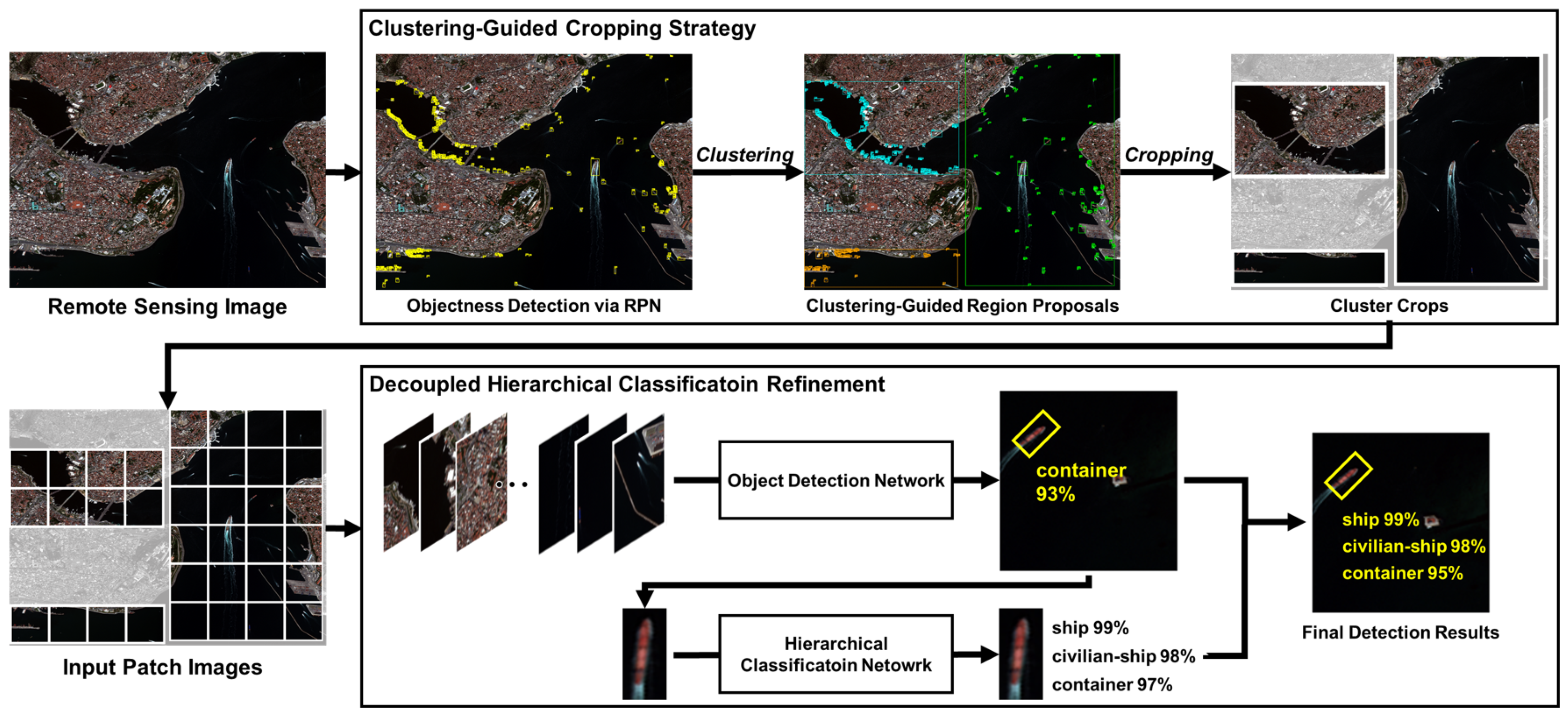
The overview of our proposed framework is illustrated in Figure 3. Inspired by the above-mentioned motivation, we first extract the regions required for object detection, which is most likely to include target objects. We call this process clustering-guided region proposal. Next, we create a series of patch images from the cluster crops in a sliding-window fashion. We then feed the patch images into our proposed hierarchical multi-label object detection pipeline. For each input patch image, we perform the inference of object detection, where the inference results are localized objects with corresponding hierarchical multi-labels.

3.2. Clustering-Guided Cropping Strategy

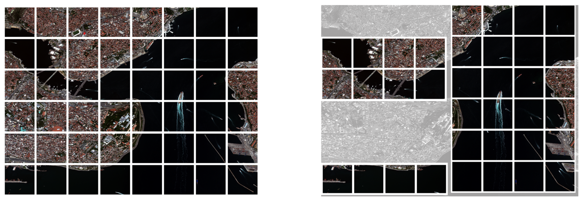
Since we cannot conjecture the approximate position of objects before inference, the existing approach tried to split the whole region of an aerial image into the set of patch images as shown in the left side of Figure 4, which we call uniform cropping throughout this paper. For example, in the case of ship detection, analyzing inland areas becomes less important compared to sea sides, island areas, or oceans with floating objects. The essence of our proposed framework is to first extract the interesting regions and then run the object detection on the extracted regions. We propose a simple yet efficient cropping strategy called clustering-guided cropping for the efficient detection, as illustrated in the right side of Figure 4.
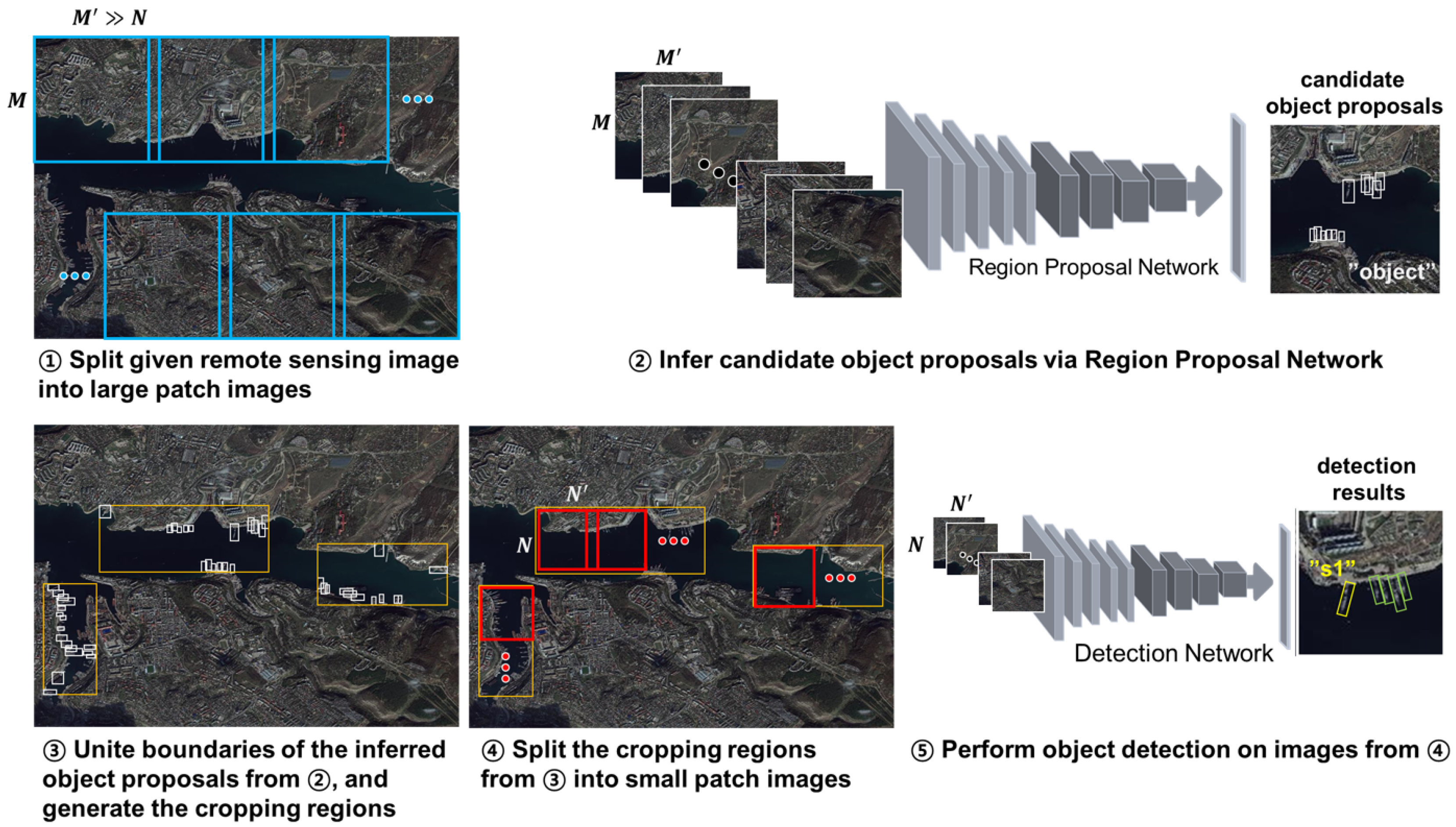
We now elaborate the design of clustering-guided cropping strategy; the overview is depicted in Figure 5. The key idea of our proposed strategy is to infer object proposals by quickly scanning input aerial image and determine the boundary of cluster crops by gathering and clustering the inferred object proposals. For generating the candidate object proposals where objects are likely to be present, we use Region Proposal Network (RPN) which is a well-known sub-network of typical two-stage detectors.
To create dataset for training and testing RPN, we split the input aerial image evenly with size M × M normally larger than the input patch size N × N of the object detector. A larger value of M leads to smaller number of split images and faster inference of RPN; however, the excessive size M would cause a deterioration of the objectness accuracy. The reason is that M × M patch should be resized to a pre-defined input size for entering into RPN, due to GPU memory constraints. As the value of M increases, the spatial resolution of the resized image is more decreased, and objects become smaller. We should set M in consideration of the speed-accuracy trade-off. With the usage of RPN that is robust to detection of small objects such as feature pyramid network (FPN), we could deal with the small object detection despite the relatively large M value. We adopt RPN for faster inference due to the lightweight structure consisting fully convolution layers, but are not limited to the usage of RPN for object proposals.
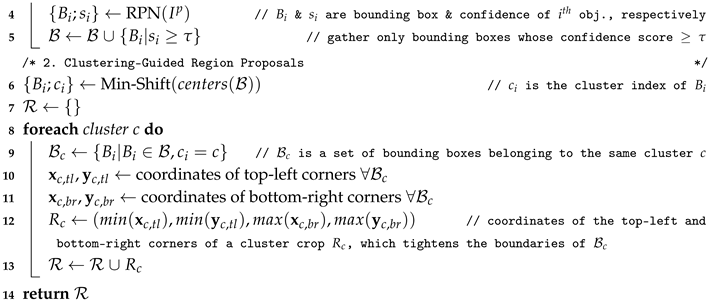
After inferring the objectness via RPN, we merge all detected objects and run min-shift clustering algorithm [15], following the clustering process of groundtruth object boxes in [16]. The min-shift clustering algorithm is a nonparametric centroid-based clustering algorithm taking the density of data instances into account, without any prior knowledge of the number of clusters. We cluster the center points of the detected boxes by the min-shift clustering algorithm, and then get the set of minimum and maximum coordinates of boxes belonging to the same cluster. Finally, we determine the boundary of each cluster crop as a pair of the minimum and maximum coordinates—the top-left corner and bottom-right corner. We split each cluster crop into the set of N × N patch images in a sliding-window manner. Later, the patch images are fed into the proposed object detection pipeline. The detailed implementation for clustering-guided cropping strategy is summarized in Algorithm 1:
Algorithm 1: Clustering-Guided Cropping Strategy
Input: a remote sensing image I, a score threshold τ
Output: coordinates of cluster crops R
/* 1. Inference of Candidate Object Proposals via RPN                          */
  • I p ← CreatePatches ( I )     
    // I is divided into a set of patch images Ip
  • B { }    
    // B is a union set of all bounding boxes on Ip inferred by RPN
  • foreachpatch image I p I p do
Remotesensing 12 02734 i001

3.3. Decoupled Hierarchical Classification Refinement

3.3.1. Pipeline Design

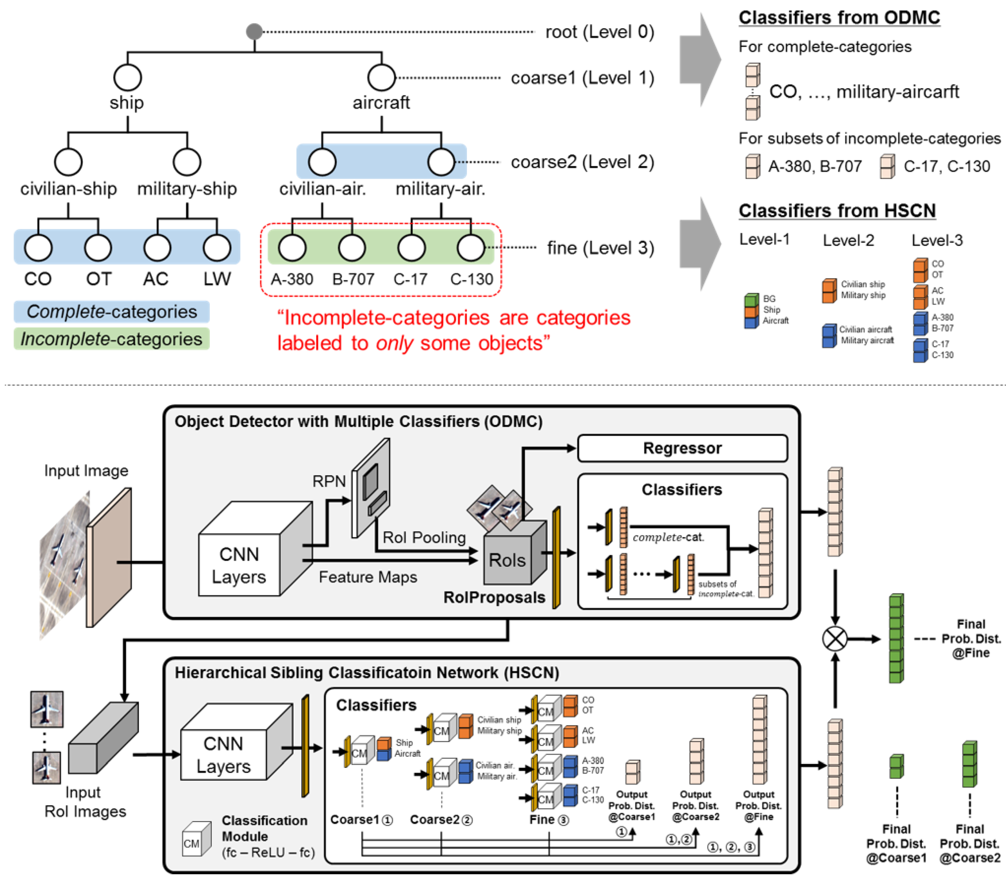
We propose a novel object detection pipeline called Decoupled Hierarchical Classification Refinement (DHCR), which explicitly adapts to hierarchically partial-annotated dataset depicted in Figure 1. We build this pipeline through combining two networks in a sequential manner as shown in Figure 6: (1) an Object Detection network with Multiple Classifiers (ODMC); (2) a Hierarchical Sibling Classification Network (HSCN). Figure 6 shows our pipeline design. The separated deployment of a detection network and a classification network is inspired by the success of decoupled classification refinement (DCR) [19]. Beyond the detection of objects labeled in a “flat” structure, we extend DCR to the hierarchical multi-label object detection.
When an input patch image is fed into ODMC, objects are detected in the form of bounding boxes with corresponding confidence scores over categories. Then, the objects are warped to a fixed size (e.g., 224 × 224) for forwarding them to HSCN, where HSCN substitutes the traditional single classification branch with multiple classification branches for outputting hierarchical multi-label classification results. The final score of HSCN for an input object combines confidence scores from all outputs of deployed classifiers. Finally, we merge the predicted probability distributions from ODMC and HSCN by element-wise multiplication.
As shown in Figure 6, we have following core modules in our proposed pipeline:
  • RoIProposals from ODMC: As a typical module in general two-stage detectors, this module generates RoIs likely to include target objects on an input patch image.
  • Regressor from ODMC: For RoIs from RoIProposals from ODMC module, this module corrects localization boxes for each RoI. After this bounding box refinement, we create input RoI images of HSCN in an upright position.
  • Classifiers from ODMC: For RoIs from RoIProposals from ODMC module, this module estimates over complete and incomplete categories at fine level based on the results from multiple classifiers. According to the predicted results of this module, false negative boxes are determined and appended to the input RoI images of HSCN.
  • Classifiers from HSCN: This module not only refines the fine-level classification result of Classifiers from ODMC module, but also predicts probability distributions over categories at each coarse level.
The common approach of ODMC and HSCN lies in replacing the single classifier with multiple parallelized classifiers. In the final layer of a typical classification module, the representative operation, e.g., SoftMax, is usually used for computing a probability distribution over all classes. In other words, the probabilities across all classes compete against each other and optimization might be biased depending on the category frequency [39]. In the case of HSCN, given the hierarchically annotated dataset where there are hierarchical relationships among classes, we partition the global competition over all classes into the local competitions between sibling classes. We can learn the classifier weights specialized in each set of sibling classes. ODMC takes more simplified approach; we define two kinds of class sets as described in the top side of Figure 6 and learn the two class sets separately.
We divide the classifiers in ODMC into two main types; (1) the SoftMax classifier over complete-categories, and (2) the sigmoid/SoftMax classifier(s) over subsets of incomplete-categories. The former classifier is a generic classifier in existing object detection networks, while the latter classifier is additionally modeled with sigmoid or SoftMax operations. In the case of the sigmoid operation, we can exploit multi-labels with not only a fine label but also its parent coarse label(s). Because of the sigmoid properties, the coarse label(s) even in complete-categories can be used without the competition burden unlike SoftMax. We devise the classification architecture of ODMC taking the hierarchically partial-annotated objects into account to enable the reasonable learning: with a single SoftMax classifier, it is not proper for simultaneously classifying over complete-categories and incomplete-categories, because complete-categories and incomplete-categories are hierarchically related, not completely exclusive.
Analogously, HSCN builds multiple classifiers instead of a single classifier. We involve the multiple classifiers for each set of sibling classes at all levels. The multiple classifiers share the same feature vector extracted from the backbone CNN network and each classifier has the same classification module; f c -ReLU- f c layers followed by SoftMax, as shown in Figure 6. The intuition behind this modeling approach is that we formulate a hierarchical multi-label classification problem as multiple flat classification problems defined over sets of sibling classes. As for the background class, we include it only in the most top classifier, i.e., the classifier over coarse1 labels, since duplicate trainings in other classifiers are unnecessary. The final output probability over a fine class is estimated by multiplying probabilities for its parent classes recursively, which more details will be further described in Section 3.3.3.

3.3.2. Training

The proposed pipeline requires a two-stage training process, where the first stage is learning ODMC, and then using the output of the first stage, HSCN is trained in the second stage sequentially. All the predicted bounding boxes including false negatives are warped to a fixed size (e.g., 224 × 224) which are fed into HSCN. If the boxes are not horizontal but rotational, then the boxes should be rotated in an upright position before warping. We re-train the boxes with the strong classifier HSCN and then support the classification prediction results by ODMC. ODMC jointly optimizes the regression and the classification, and hence may lead to sub-optimal for the respective problems [19]. We aim to make HSCN train on the misleading prediction domain generated from ODMC.
ODMC attaches additional classifier(s) to an extracted RoI-wise feature vector, which parallels the original SoftMax classifier. As mentioned in Figure 6, we divide categories into the aforementioned two types of class sets: complete-categories and incomplete-categories. ODMC separately optimizes for complete-categories and incomplete-categories by the original SoftMax classifier and the other additional classifier(s), respectively. For the newly added classifier(s), we introduce two different methods: a SoftMax classifier trained with a single label or a sigmoid classifier trained with multiple labels. We should consider the characteristics of dataset for the appropriate choice of classifier methods and the composition of the classifiers.
We use a multi-task loss to minimize the objective function for the detector of ODMC: L O D M C = L r e g + L c l s , where L r e g and L c l s are loss functions for the classification and the regression layer, respectively. Here, our classification loss function for a labeled RoI is differently defined according to the type of the classifier(s) as Equations (1),2:
With SoftMax classifier(s),
L c l s ( p α , y α , p β , y β ) = L S C E ( p α , y α ) + i λ i [ y i β C i β ] L S C E ( p i β , y i β )
with sigmoid classifier(s),
L c l s ( p α , y α , p β , y β , y p a r β ) = L S C E ( p α , y α ) + i λ i [ y i β C i β ] L B C E ( p i β , { y i β , y p a r ( i ) β } )
where S C E and B C E specify the SoftMax/sigmoid cross-entropy loss. p α , p i β denote the probability distribution over complete-categories and i t h subset of incomplete-categories, respectively. y α , y i β denote the groundtruth class belonging to complete-categories and i t h subset of incomplete-categories, respectively. If any groundtruth category of the labeled RoI does not belong to i t h subset of incomplete-categories, i.e., y i β C i β , the Iverson bracket indicator function [ y i β C i β ] evaluates to 0 and 1 otherwise. For each sigmoid classifier trainable with multi-labels, we can arbitrarily use parent classes of y i β denoted by y p a r ( i ) β , required for training the classifier. λ i is the balancing parameter for classification on i t h subset of incomplete-categories.
HSCN addresses the hierarchical multi-label classification problem by locally placing flat classification modules over the sets of sibling classes. As for the background class, we included in the most top classifier for competing only against the coarse1 labels. All localized classification modules share the same image-level feature vector as input data. The presented architecture pursues a flexible training for sub-classes without the being constrained to hierarchical dependency. We design the loss function of HSCN for each warped RoI to be a weighted summation of all SoftMax cross-entropy losses as in Equation (3).
L ( { p s , y s } s = 1 S ) = s S λ s t s L S C E ( p s , y s )
where S is the union of sets of sibling classes at all levels and s is a set of sibling classes as a subset of S. t s denotes whether a groudtruth label y belongs to s. If a groundtruth label y does not belong to s, then we cannot define y s and do not reflect corresponding loss, L S C E ( p s , y s ) by setting t s = 0 , otherwise the value t s is 1. For each sibling class group s, the SoftMax cross-entropy loss is optimized with the groundtruth label y s on the probability distribution p s . λ s is the balancing weight for the classifier over s.

3.3.3. Inference

Inference is also processed in a sequential manner. For each input image, ODMC first outputs localized objects with predicted labels by SoftMax-SoftMax classifiers or SoftMax-sigmoid classifiers. The all inferred bounding boxes of objects are warped to a fixed size. Afterwards, HSCN takes the warped bounding boxes as inputs and estimates the probability distributions over sibling classes at all levels. HSCN computes the probability for a fine label by recursively multiplication of all ancestor probabilities including itself. We obtain an unnormalized final probability distribution over all fine labels through element-wise product of the two probability distributions from ODMC and HSCN. The above all computations for probability distributions over fine labels for each labeled RoI can be expressed by the following Equations (4)–(6).
p j , L O D M C = [ y j , L C α ] p j , L α + [ y j , L C α ] p p a r ( j ) , l * α p j , L β · l = l * + 1 L 1 p p a r ( j ) , l β ·
p j , L H S C N = p j , L l = 1 L 1 p p a r ( j ) , l
p j , L D H C R p j , L O D M C · p j , L H S C N
where y j , l is the groundtruth class at level l. p j , L ( · ) is the final predicted probability given a model for y j , L . The Iverson bracket indicator functions [ y j , L C α ] and [ y j , L C α ] evaluate to 1 if the y j , L is in/not in complete-categories, respectively. p j , l β · denotes the probability for class j at level l from corresponding classifier, β · . Here, p a r ( j ) , l denotes the parent class at level of class j.

4. Experiments

To validate the contributions of the proposed framework, we conduct extensive experiments on 1) clustering-guided cropping strategy in Section 4.2 and Section 2) decoupled hierarchical classification refinement in Section 4.3. In this section, we start by explaining our datasets used for the experiments in Section 4.1, and then present implementation details and various qualitative and quantitative experimental results.

4.1. Dataset Description

We constructed two datasets with 963 WorldView-3 [12] and 457 SkySat [13] pansharpenend remote sensing images, mainly covering harbor- and airport- peripheral areas. Each remote sensing image is labeled by experts in aerial image interpretation with multiple categories, and the categories are hierarchically organized. The category hierarchy and the number of objects for each category are given in Figure 7. For WorldView-3 satellite, the images have a resolution of 0.3 m, and is of the size in the range from about 200 × 7000 to 16,000 × 16,000 pixels (sorted by their areas). For SkySat satellite, the images have a resolution of 1 m, and is of the size in the range from about 22,000 × 8000 to 23,000 × 31,000 pixels (sorted by their areas). We randomly split satellite images into 60% for training, 20% for validation, and 20% for testing on each dataset, and then create patches from all the satellite images to avoid duplicate object information being included in both training and testing patch images. In our datasets, complete-categories are CA, MA, CO, OT, MV, AC, SU, LW, and SW. The short names for the categories are defined as: CO=COntainer, OT=Oil Tanker, MV=Maritime Vessels, AC=Aircraft Carrier, SU=SUbmarine, LW=Large Warship, and SW=Small Warship. In our datasets, only some objects are annotated up to specific aircraft such as civilian aircraft (e.g., B-707, B-717, B-727, etc.) and military aircraft (e.g., A-10, A-12, A-18, etc.).

4.2. Experiments on Clustering-Guided Cropping Strategy

We perform qualitative experiments and a series of sensitivity analyses on the WorldView-3 dataset. For the qualitative experiments, we visualized some example results of cluster crops generated on the WorldView-3 test images. The sensitivity analyses are conducted to find appropriate settings for RPN and construction of patch images from the generated cluster crops.

4.2.1. Implementation Details

We use RPN of Feature Pyramid Network (FPN) (Re-implementation version publicly from https://github.com/DetectionTeamUCAS/FPN_Tensorflow) [26] for inferring candidate object proposals, which is robust to variance in scale. All input patch images are entered into RPN after resizing to 1024 × 1024 . We follow the original source code on hyper-parameters unless specified. Specifically, MomentumOptimizer [40] with momentum of 0.9 is used for optimization. We train a total of 150 k iterations, with a learning rate of 0.001 for the first 60 k iterations, 0.0001 for the next 20 k iterations, and 0.00001 for the remaining 70 k iterations. We use a 5-level pyramid levels from P2 to P6, and at each pyramid level, anchors with one scale {1.0} and three anchor ratios {0.5, 1.0, 2.0} are used. All evaluations were carried out on two TITAN Xp GPUs with 12 G memory; one GPU for ODMC, and another GPU for HSCN.

4.2.2. Qualitative Results

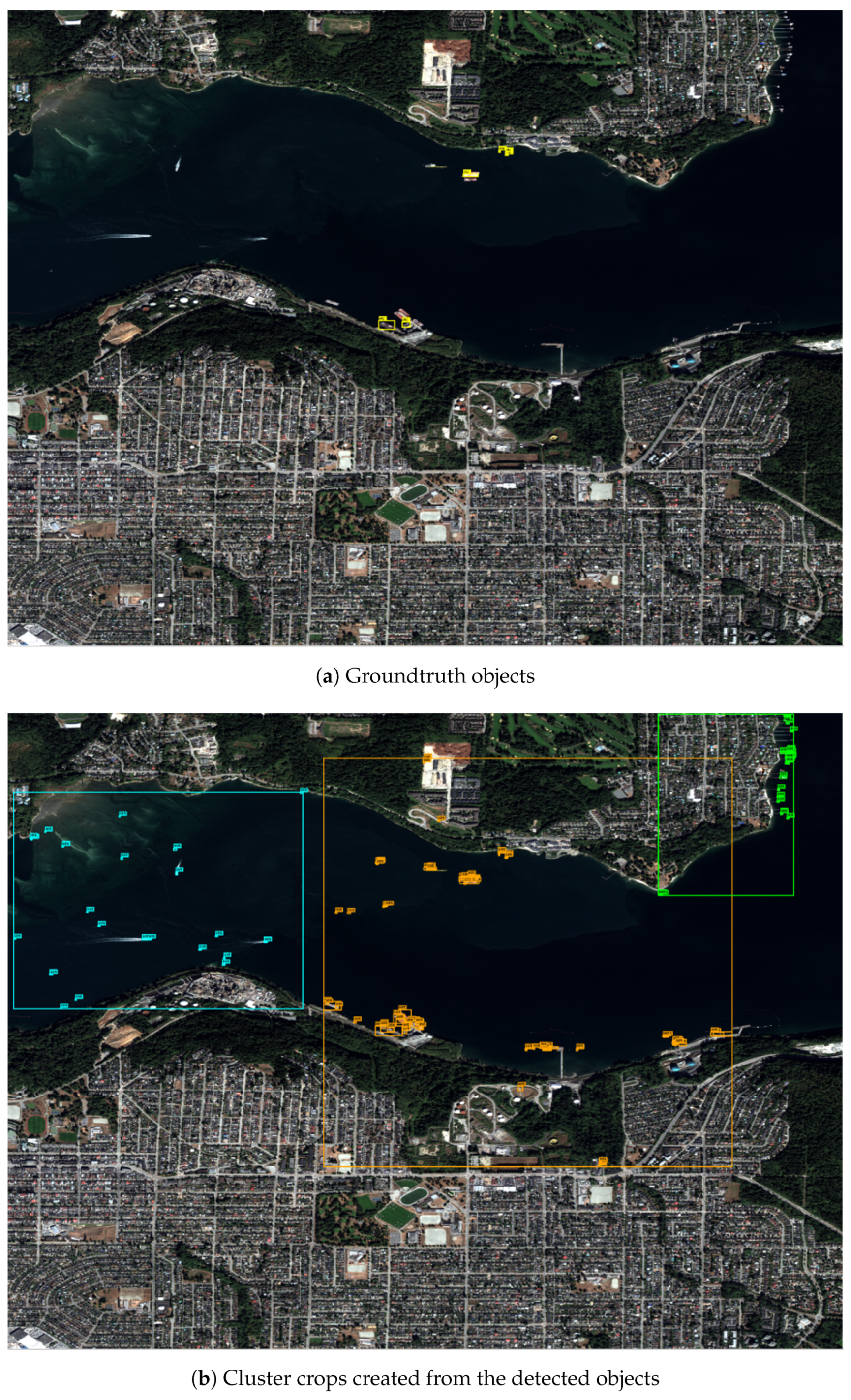
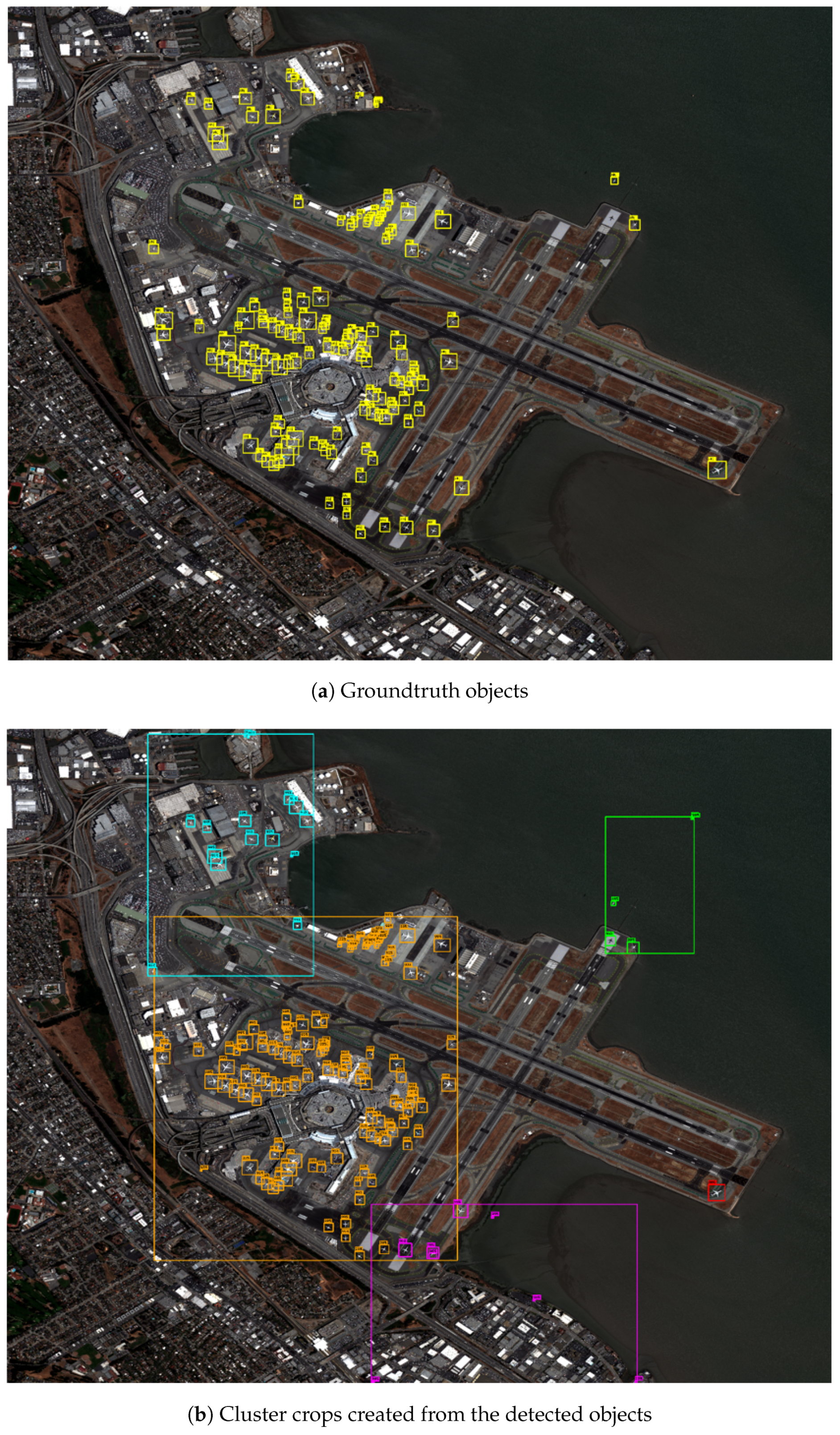
We generate cluster crops on the WorldView-3 test datasets and the results on harbor and airport peripheral areas are displayed in Figure 8 and Figure 9, respectively. The top side of each figure presents the image with the groundtruth objects represented by yellow bounding boxes. The bottom side of each figure provides the image with the detected objects and the generated cluster crops, plotted in different colors according to the clusters. We use the raw patch size of 3000 before down-scaling to a fixed input size of 1024 when training and testing RPN. For running mean-shift clustering, we only take object proposals whose objectness scores are higher than 0.985.
In the example of Figure 8, three cluster crops are generated. The regions suggested by the cluster crops are mainly spread to the sea areas including the sea shores. This experimental result fits our intuition; the target objects as ships are likely to be in certain areas such as sea sides, island areas, and oceans rather than inland areas. As shown in Figure 8a although there does not groundtruth objects in the sea shore, our RPN infers candidate object proposals due to small-scale traces which look like ships or very small ships that have not yet been unlabeled. However, as we are in the stage of the region proposal for subsequent object detection, the suggested sea shore regions are still plausible as the candidate regions to be explored. Figure 9 presents the other experimental result, which also generates three cluster crops. Many aircraft are detected as candidate object proposals especially around aerial routes.
Overall, we see that the generated cluster crops in Figure 8b and Figure 9b well capture the regions, in which the groundtruth objects are mostly situated. Massive backgrounds with very little chance of target objects being present take up many parts in the other regions that are not covered in the generated crops. Our clustering-guided cropping strategy helps saving the cost of exploring the less important regions.

4.2.3. Sensitivity Analysis

We perform the sensitivity analyses varying (1) the raw patch sizes of {3000, 5000, 7000, 9000} before down-scaling to a fixed input size of 1024 when training and testing RPN, (2) the confidence thresholds of {0.980, 0.985, 0.990, 0.995} for clustering only objects that are detected with a confidence score higher than the confidence threshold, and (3) the padding sizes of {300, 600, 900} from outside crop border line. We use four metrics and details are described as follows:
  • Number of patches to be inferred: For uniform cropping, we count the number of patches created from the whole images, while for clustering-guided cropping, we count the number of patches created from the cluster crops.
  • Number of groundtruth objects: the number of groundtruth objects included in the output cluster crops. In the case of uniform cropping, there is no loss to the groundtruth objects unless truncated.
  • Total inference time (s/img): the average running time per image from the beginning of the object detection framework until the end.
  • Average of mean Average Precision (Avg. of mAP) (%): detection performance over incomplete-categories. mAP is used as a standard metric to evaluate the performance of object detection and computed as the average value of AP over all categories. Here, AP computes the average value of precision over the interval from recall = 0 to recall = 1. The precision measures the fraction of detections that are true positives, while the recall measures the fraction of positives that are correctly identified. Hence, the higher the mAP, the better the performance.
Through the metrics, we explore the trade-off between time and memory cost (measured with the first and third metrics), and accuracy (measured with the second and fourth metrics) compared with uniform cropping. The uniform cropping illustrated in Figure 4 splits the whole region of an aerial image into the set of patch images, while clustering-guided cropping splits the regions selectively. Therefore, the clustering-guided cropping cannot completely surpass the uniform cropping statistically only in terms of accuracy. We ultimately aim at efficient object detection guided by our conjecture of regions likely to include target objects, without loss of groundtruth objects as much as possible.
The sensitivity analyses are carried out to find out the adequate hyper-parameters such as the raw patch size before down-scaling, the confidence threshold for clustering, and the padding size from outside crop border line. As the larger the raw patch size, the lower the image resolution and the smaller the object sizes. The results in Table 1a demonstrate the impact of the raw patch size, where experimental cells with 3000 × 3000 show the best mAP on average and mAP gradually degrades as the raw patch size increases. It is noteworthy that the total inference time is cut in about half on 9000 × 9000 compared to 3000 × 3000 while the average performance only drops by 2.69%. From Table 1b, we can see that the confidence threshold is another influential factor. The higher we set the confidence threshold, the fewer objects are taken, which leads to decreasing the total runtime but causing performance drop because the likelihood of losing groundtruth objects is getting higher. In the case of the third sensitivity analysis in Table 1c, we differentiate the padding size by 300, 600, and 900; since the region proposals tighten the boundaries of the clustered object proposals, we reserve margins through the paddings so as to relax the dependency on inferred object boundaries. The adequate padding size obviously may help to improve the performance; however at least in our experiments, it yields gaps that are not that large.
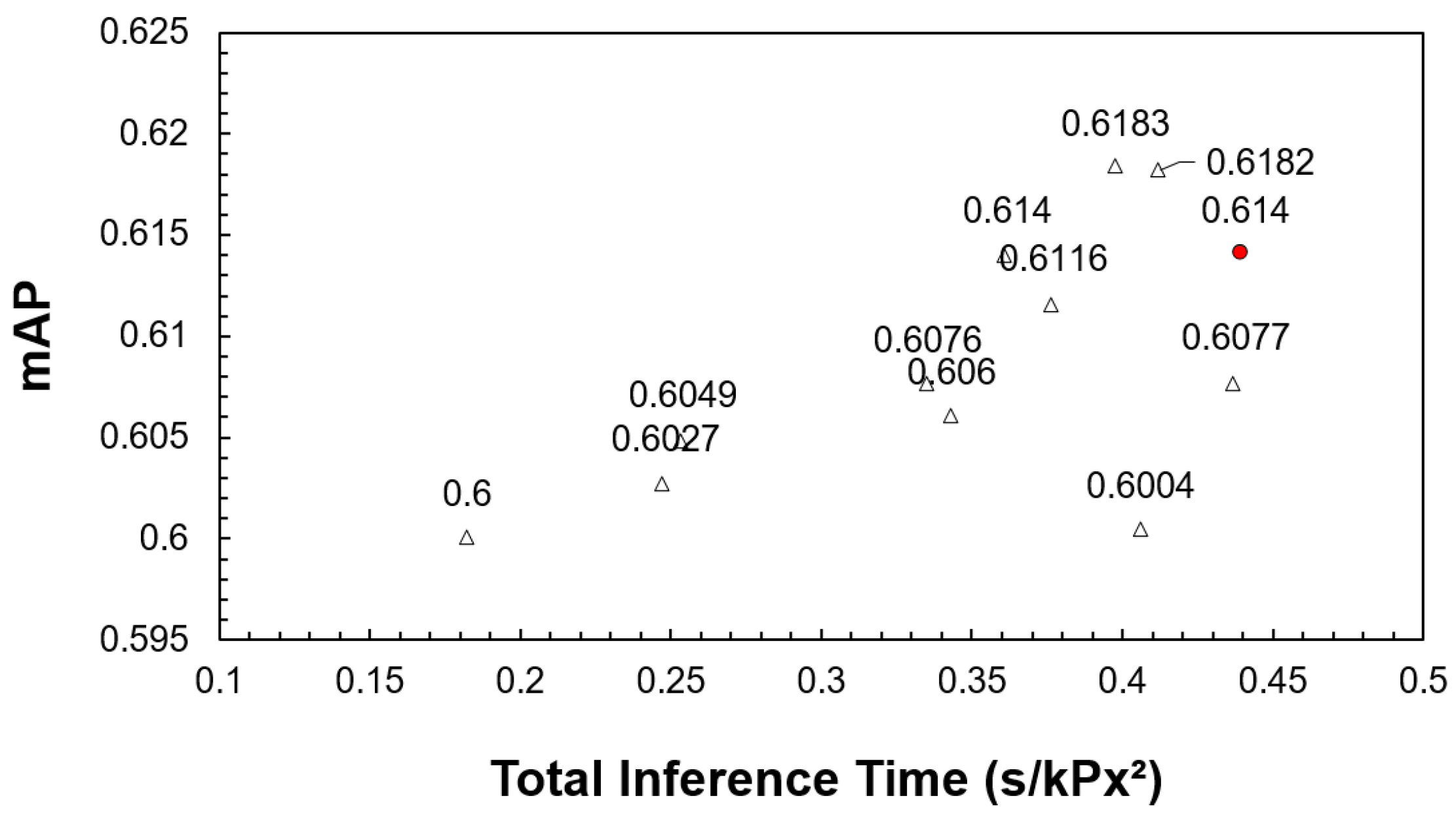
We investigate top-N experimental cells by sorting in descending order of their detection performance, mAP, and plot the speed/accuracy trade-off curve in Figure 10. From Figure 10, we see that the total inference time steadily consumes, mAP values increase and are approaching mAP of uniform cropping. Although some experimental cells show similar performance as the uniform cropping, there are comparative benefits in terms of the total inference time. For some experimental cells surpassing mAP of the uniform cropping, we simply attribute the small gaps with the uniform cropping to difference in input data distribution.

4.3. Experiments on Decoupled Hierarchical Classification Refinement

Considering a wide range of object scales of WorldView-3 and SkySat satellite images, we apply a multi-scale testing at the inference stage, and use testing scales of {768, 1024, 2048} with corresponding strides of {192, 256, 512}. The raw patch images of different sizes are then resized to have fixed sizes, 768 × 768, for entering the detection networks. The SoftMax operations are used in all the classifiers.

4.3.1. Baselines

Due to the characteristics of the aerial images, rotational bounding boxes are more suitable to encompass the objects and distinguish crowded objects from each other rather than horizontal bounding boxes [41,42]. We choose rotational object detection networks as baselines; (1) Rotation Region Proposal Networks (RRPN) [43] which learns with inclined rectangle proposals, (2) Rotational Region CNN (R2CNN) [44] which estimates both the axis-aligned box and the inclined minimum area box using different pooled features, (3) Detector for Small, Cluttered and Rotated objects (SCRDet) [45] which introduces a sampling fusion network, and pixel/channel attention networks, (4) a simple one-stage dense detector called RetinaNet [46] which optimizes focal loss, and 5) Rotated bounding BOX-based CNN (RBox-CNN) [47] which is based on rotation anchors and implements stable regression. All baseline detectors typically have a single SoftMax classifier at the end of each detection network. We learn the SoftMax classifier only over complete-categories. The SoftMax classifier is not proper for simultaneously classifying over complete-categories and incomplete-categories, because complete-categories and incomplete-categories are hierarchically dependent, not completely exclusive.

4.3.2. Implementation Details

We use the publicly released implementations for baseline models of RRPN (https://github.com/DetectionTeamUCAS/RRPN_Faster-RCNN_Tensorflow), R2CNN (https://github.com/DetectionTeamUCAS/R2CNN_Faster-RCNN_Tensorflow), SCRDet (https://github.com/DetectionTeamUCAS/R2CNN-Plus-Plus_Tensorflow), RetinaNet (https://github.com/DetectionTeamUCAS/RetinaNet_Tensorflow_Rotation), and RBox-CNN (https://github.com/SIAnalytics/simplified_rbox_cnn), where these models are implemented based on TensorFlow [48] framework. For all baseline models except for RetinaNet, we unify the backbone networks into ResNet-101 [49], feed input images sized of 768 × 768 , and adopt the pre-trained weights on DOTA [9] that are publicly available (https://github.com/DetectionTeamUCAS/Models). When using RetinaNet, we adopt ResNet-50 [49] as backbone network, take input images sized of 592 × 592 , and finetune over the pre-trained models (https://github.com/DetectionTeamUCAS/RetinaNet_Tensorflow_Rotation) on ImageNet. We follow the original source code on hyper-parameters unless specified.
For implementation of ODMCs, we use each baseline as a main body of ODMC and classification modules of the baselines are tailored to ODMC. We then build corresponding DHCR for each ODMC and each HSCN is trained with all the predicted bounding boxes from ODMC, including its false negatives. All bounding boxes are warped to a fixed size as 224 × 224 and then fed into HSCN. For the experiments, we constitute the classification branches of ODMCs as (1) a SoftMax classifier over complete-categories, and (2) a SoftMax classifier over incomplete-categories. We implement HSCN based on the TensorFlow-Slim classification network (https://github.com/tensorflow/models/tree/master/research/slim). As with ODMCs, we replace the single SoftMax classifier in the downloaded source code with multiple SoftMax classifiers over the sets of sibling categories at all levels. All HSCN models are learned by stochastic gradient descent (SGD) optimizer and we train a total of 600 k iterations with a learning rate of 0.0005.

4.3.3. Quantitative Results

Table 2 and Table 3 demonstrate the effectiveness of DHCR over different backbones and frameworks. We present the experiments on WorldView-3 and SkySat datasets. Without the help of DHCR, the existing baseline models with a single classifier limit to classifying in a flat N-way over complete-categories such as CA, MA, CO, OT, MV, AC, SU, LW, and SW in our dataset. The other classes at the fine level are partially annotated to some objects, and therefore the objects are learned with their corresponding coarse2 labels. In order to compute the AP values for classes not belonging to complete-categories like S and A at coarse1 label, and CS and MS at coarse2 label, we intentionally summed the children probabilities for a parent class and assume the summed value as the probability of the parent class, e.g., p ( C S ) = p ( C O ) + p ( O T ) + p ( M V ) .
As can be seen in Table 2 and Table 3, DHCR-based detections significantly improve the performance of the respective baseline models. In the proposed pipeline named DHCR, the embedded detector is able to classify into multiple labels across different sets of labels and the accompanying classifier named HSCN plays an important role in improving the performance of detection. After applying DHCR to each baseline detection model, the level-wise performance (mAP at L1/L2/L3) are all further improved on WorldView-3 dataset: from 63.58/54.43/45.05 to 66.10/55.46/53.57 for RRPN, from 64.17/56.62/47.99 to 73.01/60.58/58.12 for R2CNN, from 64.74/58.27/48.37 to 74.75/61.76/58.25 for SCRDet, from 69.53/61.92/52.33 to 81.15/69.27/63.30 for RBox-CNN, and from 62.50/53.46/44.72 to 65.10/54.41/52.15 for RetinaNet. Experimental results on SkySat dataset also show similar patterns of the performance improvement. The full model with RBox-CNN and DHCR achieves the best performance. Most importantly, thanks to the flexible and general design of the proposed pipeline called DHCR, it is adaptable to any dataset with annotations with an arbitrary hierarchical structure and can be expected to enhance the performance by usage of the hierarchy information.

4.3.4. Qualitative Results

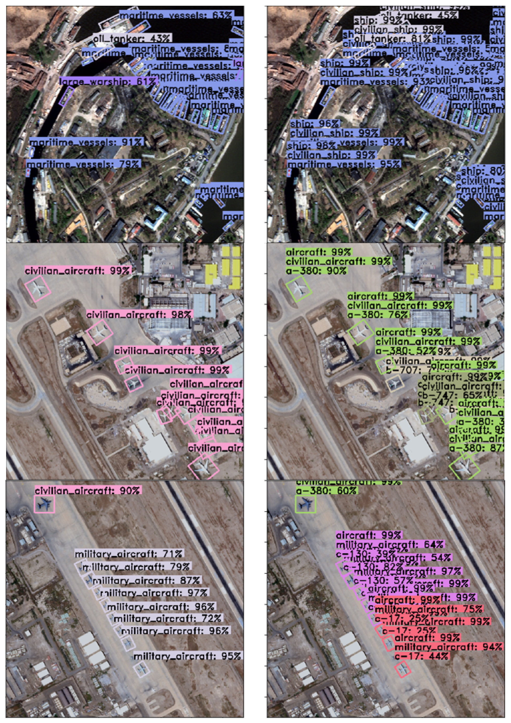
In Figure 11 and Figure 12, we visualize detection results on the WorldView-3 and SkySat test images, respectively. The detection results on both datasets commonly show substantial improvement in overall confidence scores of the true positives and detects objects with hierarchical multi-labels. Although only a few objects are labeled up to specific aircraft throughout our datasets, we could prevent a biased learning to major classes due to the key design factor in HSCN that locally deploys the classification modules. As shown in the right columns of Figure 11 and Figure 12, our pipeline presents the hierarchical multi-label object detection results, which provides much semantic and interpretable information about the objects.

5. Discussion

When we create input patch images of RPN, we must crop each huge scene image into lots of patches sized M. It is recommended that the hyper-parameter, M, be set to the value over the interval from the actual input size of RPN and to the overall scene size. A lower value of the actual input size of RPN leads to the slower speed and less efficient inference, and a higher value of the overall scene size results in including unnecessary empty areas and degrading the detection performance. In our case, the actual input size of RPN is 1,024 and the overall scene size is about 10,000. Therefore, we test M with diverse values from 3,000 to 9,000. Table 4 shows the effect of the raw input size, M, on the performance of RPN and total computational times for the training and inference process of DHCR. The hyper-parameter setting of M to a large value reduces the number of training and testing patch images generated from each scene image, which obviously brings about decreasing the computational times and declining the detection performance.
Together with Table 4, we also evaluate the average running time per patch image sized 768 × 768 for time complexity analysis among baseline models and ours in Table 5. As expected, the representative model of the one-stage detection model, RetinaNet [46], is the fastest, followed by RRPN [43], R2CNN [44], SCRDet [45], and RBox-CNNN [47]. Compared to baseline models, our model is measured as the slowest one because the backbone of ODMC is set to RBox-CNN showing the best detection performance in our experiments and we additionally perform the hierarchical classification refinement through the inference of HSCN.
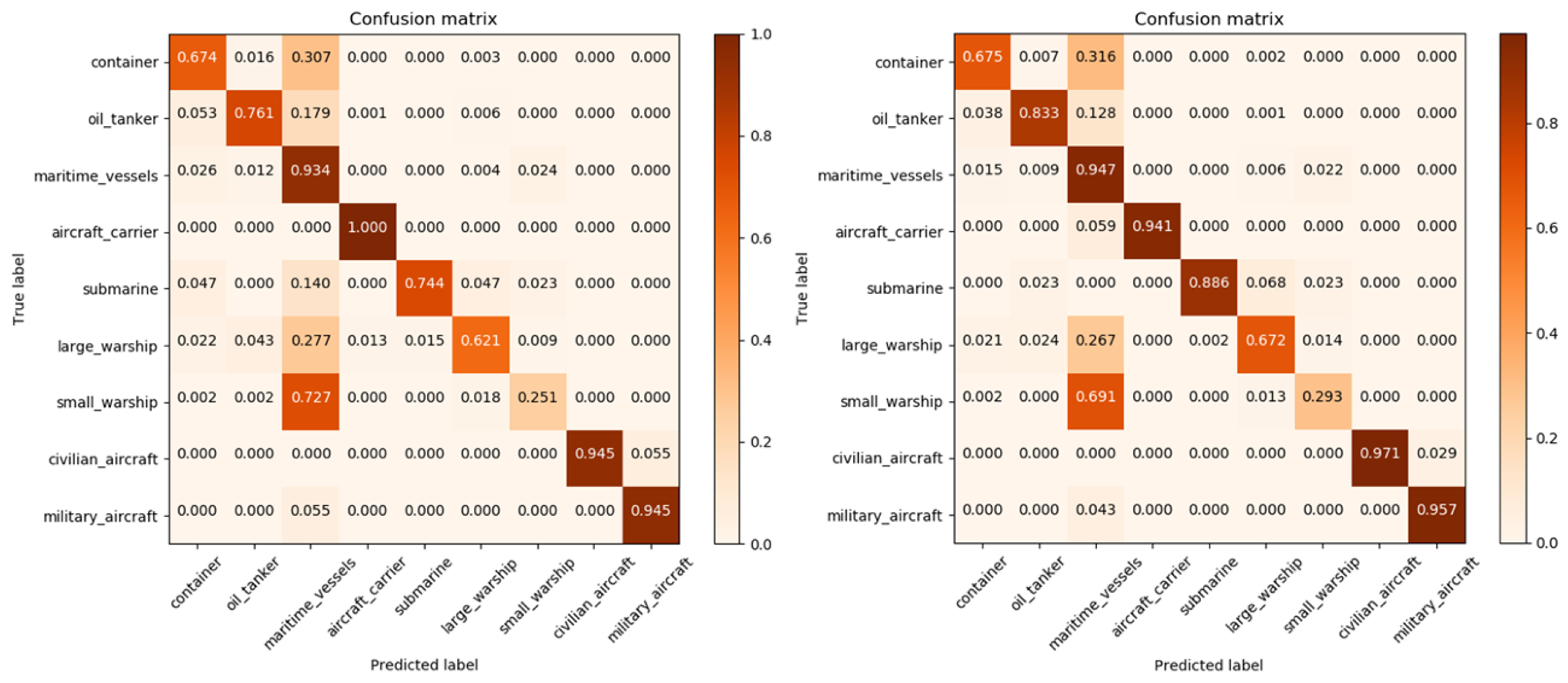
Figure 13 shows the comparison of confusion matrices before (left) and after (right) the hierarchical classification refinement. In other words, the left result is achieved after the inference of only ODMC and the right result is obtained from DHCR which fuses the results of ODMC and HSCN. As shown in the right side of Figure 13, the detection scores for the overall categories are improved after reflecting the results of HSCN, which visually provides the quantitative contribution of HSCN.

6. Conclusions

We have presented a flexible and general framework for hierarchical multi-label object detection for remote sensing images. The framework extracts crucial regions to be inferred in the subsequent object detection process on input aerial images via our clustering-guided cropping strategy, and then performs hierarchical multi-label object detection on the extracted regions by our detection pipeline called decoupled hierarchical classification refinement (DHCR). DHCR fuses the results of two networks: (1) an Object Detection network with Multiple Classifiers (ODMC), and (2) a Hierarchical Sibling Classification Network (HSCN) for supporting hierarchical multi-label classification. Due to the flexible and general design of the proposed pipeline, it is adaptable to any dataset with annotations with an arbitrary hierarchical structure. Our method shows significant improvements over several rotational detection baselines on our own two datasets constructed from WorldView-3 and SkySat satellite images. Hence, it demonstrates a practical solution for cropping regions and detecting objects with arbitrary hierarchically partial-annotated datasets. The current flexible and general design, however, requires users to adjust the model structure such as the specific determination of classification modules depending on the labeled classes of dataset, which needs to be further improved for convenient usage. As a future work, for much more realistic scenarios, we plan to further improve our proposed framework to address domain adaptation across image datasets from different satellites.

Author Contributions

Conceptualization, all authors; methodology, all authors; validation, all authors; formal analysis, all authors; investigation, S.-J.S., S.K. (Seyeob Kim) and Y.K.; resources, S.K. (Sungho Kim); data curation, S.-J.S. and S.K. (Seyeob Kim); writing–original draft preparation, S.-J.S.; writing–review and editing, S.K. (Seyeob Kim), Y.K. and S.K. (Sungho Kim); visualization, S.-J.S.; supervision, S.K. (Sungho Kim); project administration, S.K. (Sungho Kim). All authors have read and agreed to the published version of the manuscript.

Funding

This research received no external funding.

Conflicts of Interest

The authors declare no conflict of interest.

References

  1. Ahmad, K.; Pogorelov, K.; Riegler, M.; Ostroukhova, O.; Halvorsen, P.; Conci, N.; Dahyot, R. Automatic detection of passable roads after floods in remote sensed and social media data. Signal Process. Image Commun. 2019, 74, 110–118. [Google Scholar] [CrossRef] [Green Version]
  2. Fu, K.; Li, Y.; Sun, H.; Yang, X.; Xu, G.; Li, Y.; Sun, X. A ship rotation detection model in remote sensing images based on feature fusion pyramid network and deep reinforcement learning. Remote Sens. 2018, 10, 1922. [Google Scholar] [CrossRef] [Green Version]
  3. Safonova, A.; Tabik, S.; Alcaraz-Segura, D.; Rubtsov, A.; Maglinets, Y.; Herrera, F. Detection of fir trees (Abies sibirica) damaged by the bark beetle in unmanned aerial vehicle images with deep learning. Remote Sens. 2019, 11, 643. [Google Scholar] [CrossRef] [Green Version]
  4. Tuermer, S.; Kurz, F.; Reinartz, P.; Stilla, U. Airborne vehicle detection in dense urban areas using HoG features and disparity maps. IEEE J. Sel. Top. Appl. Earth Obs. Remote Sens. 2013, 6, 2327–2337. [Google Scholar] [CrossRef]
  5. Zhong, J.; Lei, T.; Yao, G. Robust vehicle detection in aerial images based on cascaded convolutional neural networks. Sensors 2017, 17, 2720. [Google Scholar] [CrossRef] [Green Version]
  6. Munir, N.; Awrangjeb, M.; Stantic, B. An Automated Method for Individual Wire Extraction from Power Line Corridor using LiDAR Data. In Proceedings of the 2019 Digital Image Computing: Techniques and Applications (DICTA), Perth, Australia, 2–4 December 2019; IEEE: Piscataway, NJ, USA, 2019; pp. 1–8. [Google Scholar]
  7. Awrangjeb, M.; Siddiqui, F.U. A new mask for automatic building detection from high density point cloud data and multispectral imagery. ISPRS Ann. Photogramm. Remote Sens. Spat. Inf. Sci. 2017, 4, 89. [Google Scholar] [CrossRef] [Green Version]
  8. Zhang, F.; Du, B.; Zhang, L.; Xu, M. Weakly supervised learning based on coupled convolutional neural networks for aircraft detection. IEEE Trans. Geosci. Remote Sens. 2016, 54, 5553–5563. [Google Scholar] [CrossRef]
  9. Xia, G.S.; Bai, X.; Ding, J.; Zhu, Z.; Belongie, S.; Luo, J.; Datcu, M.; Pelillo, M.; Zhang, L. DOTA: A large-scale dataset for object detection in aerial images. In Proceedings of the IEEE Conference on Computer Vision and Pattern Recognition, Salt Lake City, UT, USA, 18–22 June 2018; pp. 3974–3983. [Google Scholar]
  10. Liu, Z.; Wang, H.; Weng, L.; Yang, Y. Ship rotated bounding box space for ship extraction from high-resolution optical satellite images with complex backgrounds. IEEE Geosci. Remote Sens. Lett. 2016, 13, 1074–1078. [Google Scholar] [CrossRef]
  11. Cheng, G.; Zhou, P.; Han, J. Learning rotation-invariant convolutional neural networks for object detection in VHR optical remote sensing images. IEEE Trans. Geosci. Remote Sens. 2016, 54, 7405–7415. [Google Scholar] [CrossRef]
  12. DigitalGlobe. Available online: http://www.digitalglobe.com/ (accessed on 1 July 2020).
  13. Planet Labs. Available online: https://www.planet.com/ (accessed on 1 July 2020).
  14. Lin, Q.; Zhao, J.; Tong, Q.; Zhang, G.; Yuan, Z.; Fu, G. Cropping Region Proposal Network Based Framework for Efficient Object Detection on Large Scale Remote Sensing Images. In Proceedings of the 2019 IEEE International Conference on Multimedia and Expo (ICME), Shanghai, China, 8–12 July 2019; IEEE: Piscataway, NJ, USA, 2019; pp. 1534–1539. [Google Scholar]
  15. Comaniciu, D.; Meer, P. Mean shift: A robust approach toward feature space analysis. IEEE Trans. Pattern Anal. Mach. Intell. 2002, 24, 603–619. [Google Scholar] [CrossRef] [Green Version]
  16. Yang, F.; Fan, H.; Chu, P.; Blasch, E.; Ling, H. Clustered object detection in aerial images. In Proceedings of the IEEE International Conference on Computer Vision, Seoul, Korea, 27 October–2 November 2019; pp. 8311–8320. [Google Scholar]
  17. Yan, Z.; Zhang, H.; Piramuthu, R.; Jagadeesh, V.; DeCoste, D.; Di, W.; Yu, Y. HD-CNN: Hierarchical deep convolutional neural networks for large scale visual recognition. In Proceedings of the IEEE International Conference on Computer Vision, Santiago, Chile, 7–13 December 2015; pp. 2740–2748. [Google Scholar]
  18. Ouyang, W.; Wang, X.; Zhang, C.; Yang, X. Factors in Finetuning deep model for object detection with long-tail distribution. In Proceedings of the IEEE Conference on Computer Vision and Pattern Recognition, Las Vegas, NV, USA, 27–30 June 2016; pp. 864–873. [Google Scholar]
  19. Cheng, B.; Wei, Y.; Shi, H.; Feris, R.; Xiong, J.; Huang, T. Revisiting rcnn: On awakening the classification power of faster rcnn. In Proceedings of the European Conference on Computer Vision (ECCV), Mubich, Germnay, 8–14 September 2018; pp. 453–468. [Google Scholar]
  20. Ammour, N.; Alhichri, H.; Bazi, Y.; Benjdira, B.; Alajlan, N.; Zuair, M. Deep learning approach for car detection in UAV imagery. Remote Sens. 2017, 9, 312. [Google Scholar] [CrossRef] [Green Version]
  21. Cortes, C.; Vapnik, V. Support-vector networks. Mach. Learn. 1995, 20, 273–297. [Google Scholar] [CrossRef]
  22. Audebert, N.; Le Saux, B.; Lefèvre, S. Segment-before-detect: Vehicle detection and classification through semantic segmentation of aerial images. Remote Sens. 2017, 9, 368. [Google Scholar] [CrossRef] [Green Version]
  23. Xu, Y.; Zhu, M.; Li, S.; Feng, H.; Ma, S.; Che, J. End-to-end airport detection in remote sensing images combining cascade region proposal networks and multi-threshold detection networks. Remote Sens. 2018, 10, 1516. [Google Scholar] [CrossRef] [Green Version]
  24. Chen, F.; Ren, R.; Van de Voorde, T.; Xu, W.; Zhou, G.; Zhou, Y. Fast automatic airport detection in remote sensing images using convolutional neural networks. Remote Sens. 2018, 10, 443. [Google Scholar] [CrossRef] [Green Version]
  25. Yang, X.; Sun, H.; Fu, K.; Yang, J.; Sun, X.; Yan, M.; Guo, Z. Automatic ship detection in remote sensing images from google earth of complex scenes based on multiscale rotation dense feature pyramid networks. Remote Sens. 2018, 10, 132. [Google Scholar] [CrossRef] [Green Version]
  26. Lin, T.Y.; Dollár, P.; Girshick, R.; He, K.; Hariharan, B.; Belongie, S. Feature pyramid networks for object detection. In Proceedings of the IEEE Conference on Computer Vision and Pattern Recognition, Honolulu, HI, USA, 21–26 July 2017; pp. 2117–2125. [Google Scholar]
  27. Chen, Z.; Zhang, T.; Ouyang, C. End-to-end airplane detection using transfer learning in remote sensing images. Remote Sens. 2018, 10, 139. [Google Scholar] [CrossRef] [Green Version]
  28. Li, W.; Fu, H.; Yu, L.; Cracknell, A. Deep learning based oil palm tree detection and counting for high-resolution remote sensing images. Remote Sens. 2017, 9, 22. [Google Scholar] [CrossRef] [Green Version]
  29. Pang, J.; Li, C.; Shi, J.; Xu, Z.; Feng, H. R2-CNN: Fast Tiny Object Detection in Large-scale Remote Sensing Images. IEEE Trans. Geosci. Remote Sens. 2019, 57, 5512–5524. [Google Scholar] [CrossRef] [Green Version]
  30. Li, C.; Yang, T.; Zhu, S.; Chen, C.; Guan, S. Density Map Guided Object Detection in Aerial Images. In Proceedings of the IEEE/CVF Conference on Computer Vision and Pattern Recognition Workshops, Seattle, WA, USA, 13–19 June 2020; pp. 190–191. [Google Scholar]
  31. Redmon, J.; Farhadi, A. YOLO9000: Better, faster, stronger. In Proceedings of the IEEE Conference on Computer Vision and Pattern Recognition, Honolulu, HI, USA 21–26 July 2017; pp. 7263–7271. [Google Scholar]
  32. Zhu, X.; Bain, M. B-CNN: Branch convolutional neural network for hierarchical classification. arXiv 2017, arXiv:1709.09890. [Google Scholar]
  33. Parag, T.; Wang, H. Multilayer Dense Connections for Hierarchical Concept Classification. arXiv 2020, arXiv:2003.09015. [Google Scholar]
  34. Redmon, J.; Divvala, S.; Girshick, R.; Farhadi, A. You only look once: Unified, real-time object detection. In Proceedings of the IEEE Conference on Computer Vision and Pattern Recognition, Las Vegas, NV, USA, 26 June–1 July 2016; pp. 779–788. [Google Scholar]
  35. Redmon, J.; Farhadi, A. Yolov3: An incremental improvement. arXiv 2018, arXiv:1804.02767. [Google Scholar]
  36. Hussain, T.; Muhammad, K.; Del Ser, J.; Baik, S.W.; de Albuquerque, V.H.C. Intelligent Embedded Vision for Summarization of Multiview Videos in IIoT. IEEE Trans. Ind. Informatics 2019, 16, 2592–2602. [Google Scholar] [CrossRef]
  37. Hussain, T.; Muhammad, K.; Ullah, A.; Cao, Z.; Baik, S.W.; de Albuquerque, V.H.C. Cloud-assisted multiview video summarization using CNN and bidirectional LSTM. IEEE Trans. Ind. Informatics 2019, 16, 77–86. [Google Scholar] [CrossRef]
  38. Nair, V.; Hinton, G.E. Rectified linear units improve restricted boltzmann machines. In Proceedings of the 27th International Conference on Machine Learning (ICML-10), Haifa, Israel, 21–24 June 2010. [Google Scholar]
  39. Tan, J.; Wang, C.; Li, B.; Li, Q.; Ouyang, W.; Yin, C.; Yan, J. Equalization Loss for Long-Tailed Object Recognition. In Proceedings of the IEEE/CVF Conference on Computer Vision and Pattern Recognition, Seattle, WA, USA, 13–19 June 2020; pp. 11662–11671. [Google Scholar]
  40. Ruder, S. An overview of gradient descent optimization algorithms. arXiv 2016, arXiv:1609.04747. [Google Scholar]
  41. Yang, X.; Sun, H.; Sun, X.; Yan, M.; Guo, Z.; Fu, K. Position detection and direction prediction for arbitrary-oriented ships via multitask rotation region convolutional neural network. IEEE Access 2018, 6, 50839–50849. [Google Scholar] [CrossRef]
  42. Ding, J.; Xue, N.; Long, Y.; Xia, G.S.; Lu, Q. Learning RoI transformer for oriented object detection in aerial images. In Proceedings of the IEEE Conference on Computer Vision and Pattern Recognition, Long Beach, CA, USA, 15–21 June 2019; pp. 2849–2858. [Google Scholar]
  43. Ma, J.; Shao, W.; Ye, H.; Wang, L.; Wang, H.; Zheng, Y.; Xue, X. Arbitrary-oriented scene text detection via rotation proposals. IEEE Trans. Multimed. 2018, 20, 3111–3122. [Google Scholar] [CrossRef] [Green Version]
  44. Jiang, Y.; Zhu, X.; Wang, X.; Yang, S.; Li, W.; Wang, H.; Fu, P.; Luo, Z. R2cnn: Rotational region cnn for orientation robust scene text detection. arXiv 2017, arXiv:1706.09579. [Google Scholar]
  45. Yang, X.; Yang, J.; Yan, J.; Zhang, Y.; Zhang, T.; Guo, Z.; Sun, X.; Fu, K. Scrdet: Towards more robust detection for small, cluttered and rotated objects. In Proceedings of the IEEE International Conference on Computer Vision, Seoul, Korea, 27 Octber–3 November 2019; pp. 8232–8241. [Google Scholar]
  46. Lin, T.Y.; Goyal, P.; Girshick, R.; He, K.; Dollár, P. Focal loss for dense object detection. In Proceedings of the IEEE International Conference on Computer Vision, Venice, Italy, 22–29 October 2017; pp. 2980–2988. [Google Scholar]
  47. Koo, J.; Seo, J.; Jeon, S.; Choe, J.; Jeon, T. RBox-CNN: Rotated bounding box based CNN for ship detection in remote sensing image. In Proceedings of the 26th ACM SIGSPATIAL International Conference on Advances in Geographic Information Systems, Seattle, WA, USA, 6–9 November 2018; pp. 420–423. [Google Scholar]
  48. Abadi, M.; Barham, P.; Chen, J.; Chen, Z.; Davis, A.; Dean, J.; Devin, M.; Ghemawat, S.; Irving, G.; Isard, M.; et al. Tensorflow: A system for large-scale machine learning. In Proceedings of the 12th {USENIX} Symposium on Operating Systems Design and Implementation ({OSDI} 16), Savannah, GA, USA, 2–4 November 2016; pp. 265–283. [Google Scholar]
  49. He, K.; Zhang, X.; Ren, S.; Sun, J. Deep residual learning for image recognition. In Proceedings of the IEEE Conference on Computer Vision and Pattern Recognition, Las Vegas, NV, USA, 26 June–1 July 2016; pp. 770–778. [Google Scholar]
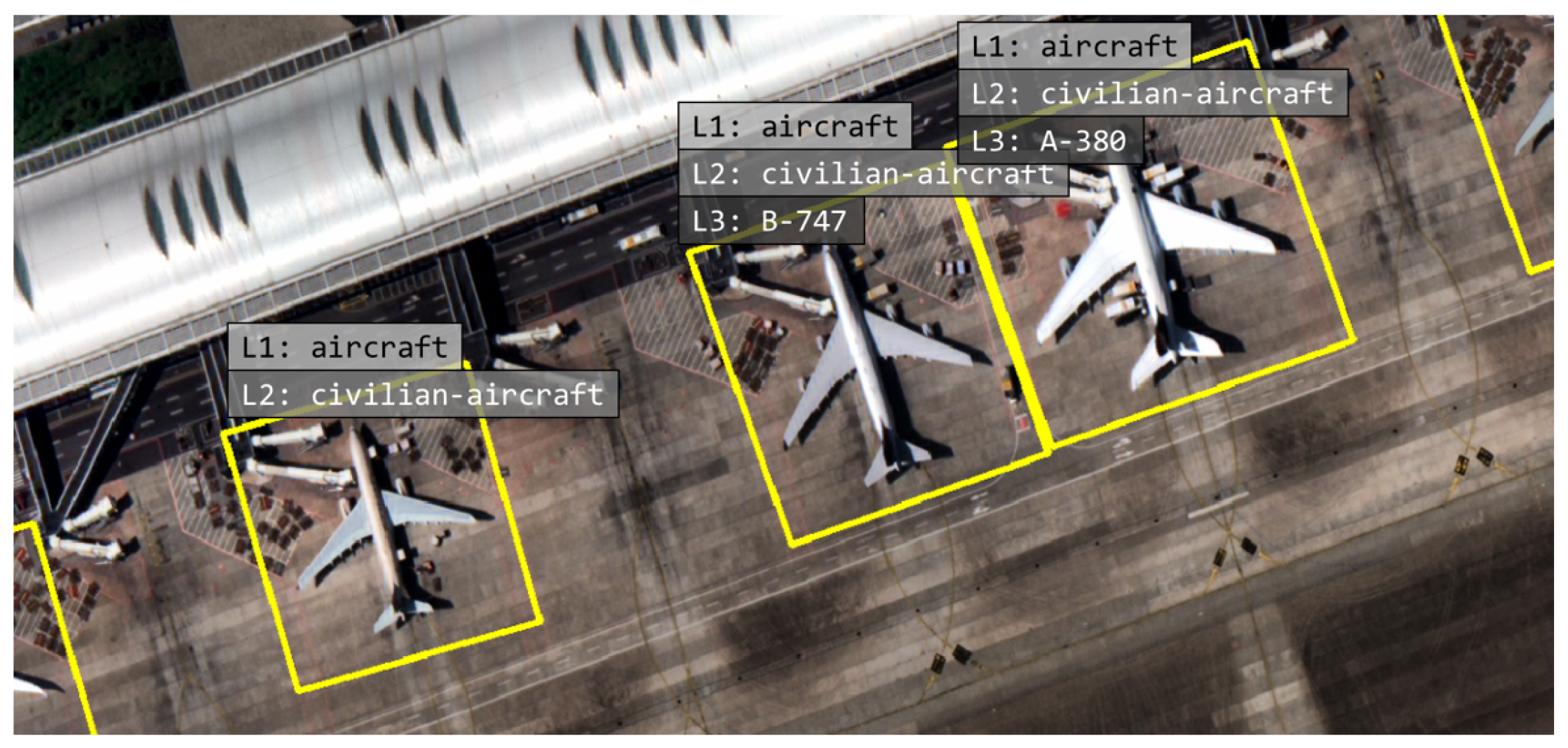
Figure 1. Demonstrative cases of annotated objects with the different labeling levels.
Remotesensing 12 02734 g001
Figure 2. Examples of large-scale remote sensing images containing sparsely distributed ship objects. The groundtruth bounding boxes are plotted in yellow color. These WorldView-3 images are provided by DigitalGlobe [12].
Remotesensing 12 02734 g002
Figure 3. Overview of the proposed hierarchical multi-label object detection framework. The interesting regions are recognized for subsequent object detection through clustering-guided region proposal. We call the regions as cluster crops and apply sliding windows from the cluster crops for acquiring input patch images. The patch images are then fed into our proposed hierarchical multi-label object detection pipeline, where the objects are detected with hierarchical multi-labels.
Remotesensing 12 02734 g003
Figure 4. Comparison of uniform cropping (left) and the proposed clustering-guided cropping (right).
Remotesensing 12 02734 g004
Figure 5. Illustration of clustering-guided cropping strategy. First, we quickly infer object proposals by Region Proposal Network. The boundary of each cluster crop is then determined by merging the inferred object proposals belonging to the same cluster. The cluster crops are re-explored by object detection networks in the form of set of patch images.
Remotesensing 12 02734 g005
Figure 6. Top: A simplified example of hierarchically partial-annotated objects with their hierarchical labels. Two types of category sets. We define two kinds of category sets called complete-categories and incomplete-categories. The complete-categories represent the set of end-labeled classes that have any ancestor which is not an end-labeled class, while the incomplete-categories denote all the descendants of complete-categories. The short names for the categories are defined as: CO=COntainer, OT=Oil Tanker, AC=Aircraft Carrier, and LW=Large Warship. Bottom: Pipeline of decoupled hierarchical classification refinement. We build this pipeline through combining two networks in a sequential manner: 1) an Object Detection network with Multiple Classifiers (ODMC); 2) a Hierarchical Sibling Classification Network (HSCN) for supporting hierarchical multi-label classification. In HSCN, we place classification modules on each sibling classifier, where a classification module is composed of fully connected (fc)-ReLU [38]-fc layers.
Remotesensing 12 02734 g006
Figure 7. Left: Distribution of objects over categories. Right: Four-depth class hierarchy of our own datasets: root at level 0 (not used), coarse1 at level 1, coarse2 at level 2, and fine at level 3. The two numbers in parentheses written below each category name mean the object counts in WorldView-3 and SkySat dataset, respectively. Only some objects are annotated as categories belonging to incomplete-categories as their fine labels.
Remotesensing 12 02734 g007
Figure 8. Example cluster crops on the satellite image taken from the harbor-peripheral areas. Each generated cluster crop and the associated object proposals are indicated by the same color. These WorldView-3 images are provided by DigitalGlobe [12].
Remotesensing 12 02734 g008
Figure 9. Example cluster crops on the satellite image taken from the airport-peripheral areas. Each generated cluster crop and the associated object proposals are indicated by the same color. These WorldView-3 images are provided by DigitalGlobe [12].
Remotesensing 12 02734 g009
Figure 10. Total inference time (s/kPx 2 ) versus detection performance (mAP) of cluster-guided cropping strategy, which explores the speed/accuracy trade-off. The plotted values are mAP of top-N experimental cells sorted in descending order of mAP. Although some top experimental cells show similar performance as the uniform cropping, we can obtain comparative benefits in terms of the total inference time.
Remotesensing 12 02734 g010
Figure 11. Comparison on the test WorldView-3 images between baseline and our proposed approach. Left column: detection results of only RBox-CNN (baseline); Right column: detection results of RBox-CNN+DHCR (ours), which shows substantial improvement in overall confidence scores and detects objects with hierarchical multi-labels. These WorldView-3 images are provided by DigitalGlobe [12].
Remotesensing 12 02734 g011
Figure 12. Comparison on the test SkySat images between baseline and our proposed approach. Left column: detection results of only RBox-CNN (baseline); Right column: detection results of RBox-CNN+DHCR (ours), which shows substantial improvement in overall confidence scores and detects objects with hierarchical multi-labels. These SkySat images are provided by Planet Labs [13].
Remotesensing 12 02734 g012
Figure 13. Comparison of confusion matrices before (left) and after (right) the hierarchical classification refinement. In other words, the left result is achieved after the inference of only ODMC and the right result is obtained from DHCR which fuses the results of ODMC and HSCN. For the overall categories, the detection score is improved after reflecting the results of HSCN.
Remotesensing 12 02734 g013
Table 1. Three types of sensitivity analyses for clustering-guided cropping strategy on WorldView-3 test dataset. We exploit RPN of Feature Pyramid Network [26] for all experiments. The symbol # denotes the number sign.
Raw Input Size (M)# Patches# GroundtruthTotal InferenceAvg. of mAP (%)
before Down-Scalingto Be InferredObjectsTime (s/img)
Uniform Cropping47,51024,37164.0761.40
3000 × 300027,80322,63445.4660.10
5000 × 500024,47721,51140.4259.28
7000 × 700023,33121,16538.7659.03
9000 × 900018,34619,58431.3357.41
a Sensitivity analysis varying the raw patch sizes before down-scaling to
a fixed input size of 1024 when training and testing RPN.
Confidence# Patches# GroundtruthTotal InferenceAvg. of mAP (%)
Threshold of RPNto be InferredObjectsTime (s/img)
Uniform Cropping47,51024,37164.0761.40
0.98025,95721,92842.3859.49
0.98524,29521,67240.0359.21
0.99022,39920,61637.4858.50
0.99519,44020,29433.4058.08
b Sensitivity analysis varying the confidence thresholds for clustering only objects
that are detected with a confidence score higher than the confidence threshold.
Padding Size# Patches# GroundtruthTotal InferenceAvg. of mAP (%)
of Cluster Cropsto be InferredObjectsTime (s/img)
Uniform Cropping47,51024,37164.0761.40
30019,07521,12733.0558.53
60022,76021,12737.8958.56
90027,23121,12744.0459.36
c Sensitivity analysis varying the padding sizes from outside crop border line.
Table 2. Detection results on WorldView-3 test set. Numbers with bold indicate the highest score, and numbers in underline indicate the second highest score on each category. Without applying DHCR, we are limited to evaluation for incomplete-categories due to a single classifier structure of existing detection models, where the single classifier is trained for complete-categories. Notations: S = Ship, A = Aircraft, CS = Civilian Ship, MA = Military Ship, CA = Civilian Aircraft, MA = Military Aircraft, CO = COntainer, OT = Oil Tanker, MV = Maritime Vessels, AC = Aircraft Carrier, SU = SUbmarine, LW = Large Warship, SW = Small Warship, For each dataset, we report the performance for certain aircraft at level3 (L3) in the order of the most frequent appearance among the various aircraft: CA 1 = A-340, CA 2 = B-757, MA 1 = AN-12, and MA 2 = C-130 in WorldView-3, and CA 1 = A-380, CA 2 = B-747, MA 1 = C-17, and MA 2 = C-130 in SkySat dataset. mAP† averages detection performance excluding CA 1 , CA 2 , MA 1 , and MA 2 at level 3.
Coarse1 Label (L1)Coarse2 Label (L2)Fine Label (L3)
Base Detector+DHCRSAmAPCSMSCAMAmAPCOOTMVACSULWSWCA 1 CA 2 MA 1 MA 2 mAP†mAP
RRPN [43]52.2374.9263.5862.7241.1270.1343.7454.4365.3853.5652.8132.9445.6835.0129.94----45.05-
R2CNN [44]53.4374.9164.1769.3642.1381.9333.0656.6270.5856.9459.0433.1746.2639.1330.81----47.99-
SCRDet [45]54.7774.7164.7469.9142.9584.5435.6758.2771.2655.6260.9934.9947.2240.4128.13----48.37-
RBox-CNN [47]64.5774.4869.5372.1244.2480.4750.8361.9270.3575.3761.3734.0450.8840.0534.24----52.33-
RetinaNet [46]51.2073.7962.5061.5741.1769.0642.0253.4664.5052.7551.0433.7543.7738.5128.71----44.72-
RRPN [45]61.8070.4066.1069.8043.9472.1835.9055.4677.1657.8558.7737.4555.6848.1739.9477.8855.1225.2240.2953.5752.14
R2CNN [43]69.7576.2773.0176.6848.9675.8940.7860.5885.4869.2055.7539.5756.2659.7640.8177.8675.5220.2250.0058.1257.31
SCRDet [44]71.7977.7074.7580.0646.5683.6636.7561.7685.9772.3258.8240.5657.2254.7438.1389.2976.5716.8845.6858.2557.83
RBox-CNN [47]81.6380.6781.1589.9351.9583.2851.9069.2793.1384.2860.1541.6560.8858.8044.2487.1470.0117.9868.4563.3062.43
RetinaNet [46]60.4569.7465.1068.5143.6671.3334.1254.4176.9056.8652.5538.9353.7747.3438.7186.4154.5324.8335.2752.1551.46
Table 3. Detection results on SkySat test set.
Coarse1 Label (L1)Coarse2 Label (L2)Fine Label (L3)
Base Detector+DHCRSAmAPCSMSCAMAmAPCOOTMVACSULWSWCA 1 CA 2 MA 1 MA 2 mAP†mAP
RRPN [43]42.4050.0146.2143.2940.0465.2030.7144.8148.6830.0932.1151.5732.0245.5428.87----38.41-
R2CNN [44]50.3254.5152.4250.5542.7564.7340.9849.7568.9036.8437.7653.2538.5746.5630.50----44.63-
SCRDet [45]49.8160.1454.9853.4440.0467.1743.6751.0868.0534.6840.8850.5940.2748.8831.05----44.91-
RBox-CNN [47]55.7570.2463.0060.0543.9980.4345.0757.3985.4545.1245.4655.1141.0553.2133.32----51.25-
RetinaNet [46]42.2351.7847.0145.2741.1266.8530.8546.0250.6631.1133.5750.9937.7645.0529.05----39.74-
RRPN [45]44.2655.4149.8448.9740.2565.4331.7846.6159.1233.4036.9956.9343.1647.7230.2971.6941.4737.636.4343.9442.26
R2CNN [43]51.8362.9257.3853.8548.9773.9935.7653.1480.6351.2941.8256.1944.2449.0731.8583.9642.1247.6319.5150.7349.85
SCRDet [44]55.4364.2359.8358.7044.7075.2334.1453.1981.6652.7644.7655.7146.1250.8833.4580.8935.9353.2520.8152.1950.57
RBox-CNN [47]61.2670.8566.0662.9750.1480.2940.5558.4990.4060.3245.8660.1247.2755.6334.7685.7935.1455.2123.8356.3454.03
RetinaNet [46]45.2357.9751.6049.3242.7870.8135.4049.5860.5935.0040.1756.5143.2446.3230.8172.4535.1940.7815.6644.6643.34
Table 4. Effect of the raw input size before down-scaling in terms of the performance of RPN and computational times for total training and inference process of DHCR.
Raw Input Size (M)Performance of RPNTraining TimeInference Time
before Down-ScalingTP Rate (%)FN Rate (%)mAP (%)(h)(s/img)
3000 × 300051.1448.8631.09218.0045.46
5000 × 500036.5263.4826.68208.0740.42
7000 × 700035.4764.5324.58195.3538.76
9000 × 900029.0470.9621.08176.1231.33
Table 5. Comparison of running times (sec/patch) for the time complexity analysis. We evaluated the running times on a patch image sized 768 × 768 with a Titan Xp GPU.
RRPN [43]R2CNN [44]SCRDet [45]RBox-CNN [47]RetinaNet [46]DHCR (Ours)
0.31340.36210.39770.45350.27990.4873