Article

Integrating RELAX with PS-InSAR Technique to Improve Identification of Persistent Scatterers for Land Subsidence Monitoring

1
College of Resource Environment and Tourism, Capital Normal University, Beijing 100048, China
2
State Key Laboratory Incubation Base of Urban Environmental Processes and Digital Simulation, Beijing 100048, China
3
Key Laboratory of 3-Dimensional Information Acquisition and Application, Ministry of Education, Beijing 100048, China
4
School of Earth, Environment and Society, Bowling Green State University, Bowling Green, OH 43403, USA
5
Beijing Laboratory of Water Resources Security, Beijing Municipal Education Commission, Beijing 100048, China
*
Author to whom correspondence should be addressed.
Remote Sens. 2020, 12(17), 2730; https://doi.org/10.3390/rs12172730
Submission received: 9 July 2020 / Revised: 17 August 2020 / Accepted: 20 August 2020 / Published: 24 August 2020

Abstract

:
Identifying Persistent Scatterers (PSs) is one of the key processing steps of the Persistent Scatterer Interferometric Synthetic Aperture Radar (PS-InSAR) technique. The number, density, and reliability of identified PSs directly affect the monitoring accuracy of land subsidence, especially in higher density urban environments. As a result of the side-looking viewing geometry of SAR, the layover effect poses a major challenge to the PS identification. This research proposes joint modeling of the PS-InSAR technique and RELAX algorithm for SAR tomography (PS-InSAR+RELAX) to detect single and double scatterers and to improve the identification and reliability of PSs. It has been demonstrated that RELAX improves separation of the scatterers when compared to two other spectral analysis methods for SAR tomography, Beam-Forming (BF) and Singular Value Decomposition (SVD). RELAX exhibits the least noise when the number of baseline changes from 15 to 30, and it can separate the scatterers at a lower Normal-Slant-Range (NSR) height than the two other methods. As RELAX can better identify, separate, and then filter out layover scatterers, the number and density of PSs identified by PS-InSAR+RELAX is reduced and visually simplified, suggesting that the method can effectively reduce the influence of the layover effect on the PS identification. Also, the PSs identified by PS-InSAR+RELAX are more coherent than those identified by the traditional PS-InSAR technique. The proposed technique has been applied to Sentinel-1A data acquired from 2014 to 2016, to monitor land subsidence in the city of Beijing, China. When evaluated against the leveling measurements, PS-InSAR+RELAX performs better than the traditional PS-InSAR technique, with the correlation coefficients (r) of r = 0.98 and r = 0.95, respectively.

Graphical Abstract

1. Introduction

Land subsidence is a geological phenomenon caused by natural physical and chemical processes or by human activities such as over-exploitation of subsurface fluids and solid minerals in synergy with construction engineering in urban areas. Land subsidence occurs in more than 150 regions and cities throughout the world [1]. The hazards due to land subsidence include damage to infrastructure and to humans [2]. To ensure sustainable urban development and the safety of people’s lives and property, land subsidence monitoring has become an ongoing process in Beijing, China.
In the past, land subsidence monitoring relied on conventional methods, which were point-based and time-consuming approaches. With the development of the Interferometric Synthetic Aperture Radar (InSAR) techniques and their capabilities to measure large-scale ground movement with an accuracy of millimeters, land subsidence monitoring has become advanced and convenient. The Persistent Scatterer Interferometric Synthetic Aperture Radar (PS-InSAR) technique, developed in recent years, overcomes the temporal and geometric decorrelation by identifying pixels in which the dominant backscattering signal is represented by a single persistent scatterer (PS) in a series of interferograms [3], which maintain high coherence, stable amplitude, and strong scattering characteristics over time [4]. Various PS-InSAR based methods have been developed and successfully used in urban areas, as high-rise buildings can be identified as PSs. The number, density, and reliability of identified PSs improve the deformation time series and deformation velocity estimated over the identified PSs and thus, improve the accuracy of displacement measurements [5]. However, the identification of PSs persists as a challenge.
Researchers have proposed several methods for identifying PSs based on the amplitude and phase information of the PS, such as phase stability analysis [6], amplitude dispersion threshold method [7], and coherence coefficient threshold method [8]. To obtain PSs with stable phase and thus to improve density of PSs, the identification process must extract most of the high-coherence pixels while reducing errors in the subsequent processing steps [7]. The PS-InSAR technique was proposed by Ferretti et al. [5,6,7]. The technique estimated deformation and residual topographic errors but was limited to the scatterers with high coherence [4]. This method was followed by the original SBAS technique [9], where small baselines and multi-looked data were used to limit the spatial correlation and reduce phase noise, respectively [4]. Another major contribution to the development of the PS-InSAR techniques was proposed by Hooper et al. in 2004, who incorporated amplitude dispersion index (ADI) as the quality indicator to identify PSs [7]. The authors used phase characteristics to identify low-amplitude targets with phase stability [7]. This method was used as the basis for the Stanford Method for Persistent Scatterers (StaMPS), a method that uses spatial correlation of interferogram phase to identify pixels with low-phase variance [3]. Since then the SqueeSAR model was developed by Ferretti et al. in 2011 [10], and other similar models developed by Goel and Adam in 2014 [11] and Devanthéry et al. in 2014 [12] (as summarized by Crosetto et al. in 2016 [4]). In addition to research on land subsidence, examples of such applications also include, landslides-related studies [13,14].
The side-looking viewing geometry of SAR triggers a major challenge in the PS identification. Adjacent building targets in urban areas affect each other, resulting in a layover phenomenon when a single pixel contain echo signals from multiple scatterers of different targets known as layover scatterers [15]. The assumption established by the PS-InSAR technique is that there is only one PS in a pixel, but in fact, in an urban environment, due to the layover phenomenon, a pixel contains two or more scatterers [5]. Therefore, the common PS-InSAR methods cannot separate these layover scatterers, and the spectral analysis methods have to be used to discriminate single from layover scatterers [2]. Nowadays SAR tomography methods offer a unique approach to solve the problem of the layover effect [16]. Furthermore, the SAR tomography methods are successfully applied to PS-InSAR, known as the Tomography-based Persistent Scatterers Interferometry (Tomo-PSInSAR) techniques, and effectively used for long-term displacement monitoring [17,18]. Generally, Tomo-PSInSAR outperforms PS-InSAR in the detection of PSs by jointly analyzing SAR amplitude and phase information [19], thus offering the advantage of increased observation samples (i.e., scattering structure) along the vertical direction. This is essential for urban areas where scattering is distributed along the structure heights [20]. Several tomography imaging methods can be used to estimate the backscattering distribution in the vertical direction. Nonparametric methods such as Beam-Forming (BF) [21], Singular Value Decomposition (SVD) [22], RELAX [23], and Capon [24], are widely used as they are flexible in collecting information from any backscattering profile [16].
In this study, we propose an innovative joint approach in which the PS-InSAR technique is combined with the spectral analysis method RELAX (PS-InSAR+RELAX) to improve the PS identification and, ultimately, the accuracy of land subsidence monitoring. Our rationale is that the selected spectral analysis method can be used to analyze the elevation-to-peak position of different types of scatterers while utilizing the spectrum characteristics of PSs and converting them to the frequency domain at the same time. To the best of our knowledge, there is no study using RELAX to identify PSs and to enhance the PS-InSAR technique for land subsidence monitoring. In addition to the detection of PSs in layover pixels, the accuracy of PSs identification is also expected to improve. The proposed PS-InSAR+RELAX technique is applied to Sentinel-1A data, acquired from 2014 to 2016, to monitor land subsidence in the city of Beijing, China. The analysis includes three parts: first, three spectral analysis methods (BF, SVD, and RELAX) are applied to Sentinel-1A data to compare their performance in identifying multi scatterers; second, the StaMPS application is used to identify PS candidates (PSC), as they contain effective PSs and layover scatterers; third, RELAX is used for the PS identifications and the PS-InSAR+RELAX and common PS-InSAR techniques are utilized to estimate and validate the land subsidence rates over the study area. Theoretical backgrounds of the PS-InSAR technique and spectral analysis methods are explained in more detail in the next section.

2. Theoretical Background

2.1. PS-InSAR Technique

In 2001, Ferretti et al. proposed the PS-InSAR technique to reduce temporal and geometric decorrelation and atmospheric influences within the traditional InSAR technique. The PS-InSAR technique selects a single master image from multiple SAR images covering the same area to form a pair of time- series interference and identifies PS with strong scattering and phase stability as the representation of land subsidence information. Based on this PS, modeling and solving are carried out to obtain subsidence information, where the effects of spatial and temporal decorrelation and atmospheric delay have been improved [7]. Based on the PS-InSAR technique, Hooper et al. developed a new method for calculating land deformation, named the StaMPS. This method works in terrains with or without buildings and no assumptions about variations in the displacement rate are required. It adopts the discrete characteristics of amplitude and the spatial correlation characteristics of the interference phase, without prior knowledge, and establishes a PS identification model based on the ADI and phase stability, which are used to identify PSs [6].
After obtaining the persistent scatterer candidates (PSC), the phase stability is analyzed and the best PSs are extracted during the processing. The basic model is defined as:
ϕ x , i = ϕ d e f , x , i + ϕ a , x , i + ϕ o r b , x , i + ϕ ε , x , i + n x , i
where ϕ x , i is the phase of the x-th PS point in the i-th interferogram, ϕ d e f , x , i is the phase related to the deformation along Line-of-Sight (LOS), ϕ a , x , i is the phase caused by the atmospheric phase, ϕ o r b , x , i is the orbit error phase, ϕ ε , x , i is digital elevation model (DEM) error phase, and n x , i is the thermal noise of the system.
The terrain phase is removed by using the external DEM. The related assumptions are that ϕ d e f , ϕ a and ϕ o r b are spatially related within a certain range of length L, ϕ ε and n are not related within this range, and that the average value is zero. The average value of all phases in a circular area with pixel x as the center and L as the radius is calculated as follows:
ϕ ¯ x , i = ϕ ¯ d e f , x , i + ϕ ¯ a , x , i + ϕ ¯ o r b , x , i
Equation (2) is subtracted from Equation (1) as follows:
ϕ x , i ϕ ¯ x , i = B , x , i K ε , x + n ¯ x , i
In Equation (3), n ¯ = ( ϕ ¯ d e f ϕ d e f ) + ( ϕ ¯ a ϕ a ) + ( ϕ ¯ o r b ϕ o r b ) , the DEM error phase ϕ ε , x , i and perpendicular baseline B , x , i are proportional and K ε , x is the scaling factor.
Using all interferograms, the least-squares method is applied to pixel x to estimate the scaling factor K ε , x . The temporal coherence γ x based on the pixel x is defined as:
γ x = 1 N | i = 1 N exp { j ( ϕ x , i ϕ ¯ x , i ϕ ^ ε , x , i ) } |
where N is the number of interferograms used, ϕ ^ ε , x , i is the estimated value of ϕ ε , x , i , assuming n ¯ ε , x , i is small, γ x is the phase stability of a pixel, and is also an indicator for determination of a PS point. Through spatio-temporal filtering, long-wavelength atmospheric effects and orbit error are removed.

2.2. Spectral Analysis Methods

Commonly-used spectral analysis methods such as Beam-Forming (BF), Singular Value Decomposition (SVD), and RELAX algorithm, are capable of estimating the backscatter distribution along the velocity plane, which make it possible to can identify and separate single and layover scatterers in a single pixel important to solve the layover phenomenon.

2.2.1. Beam-Forming (BF)

The BF spectral analysis method refers to the inversion technique of the linear relation shown in Equation (5), which models the scene complex backscattering as a function of the elevation in a selected pixel. The relationship is derived from the imaging geometry, following proper geometrical compensation [21]. It is expressed as follows:
y n = γ ( s ) exp [ j 2 π ξ n s ] d s
where yn is the signal in a fixed pixel (i, j) in the nth image; γ ( s ) is the function that models the scene complex backscattering as a function of the elevation in the selected pixel S (orthogonal to the azimuth and range plane); ξ n is the elevation spatial frequencies and given by:
ξ n = 2 b n / ( λ r )
where b n is the orthogonal baseline component of the nth pass, and λ is the operating wavelength. The measured data are generally non-uniformly-spaced samples of the spectrum of the unknown elevation scattering profile. The reconstruction of the unknown function γ ( s ) is reached by inverting the “irregular” Fourier transform operator shown in Equation (5).
From the non-uniformly-distributed samples, the elevation range can be identified as an upper limit of the backscattering distribution along the elevation. In irregular sampling, this unambiguous elevation range can be approximated as:
2 a nyq = λ r / 2 b
where b is the mean orthogonal baseline separation. The final elevation resolution of BF cannot exceed the following value:
δ S = λ r / 2 B = 2 a nyq / N
where B is the total orthogonal baseline span.

2.2.2. Singular Value Decomposition (SVD)

As an alternative to BF, some literature proposes several innovative and more robust techniques that allow moving from the data stack to the elevation scattering profile; they are either framed in the context of spatial-spectral estimation or linear inverse problems [25]. Such approaches effectively overcome the limitations regarding the non-uniformly-distributed samples, and limited number of images, which may cause poor resolution, high sidelobes, and leakage in the elevation point spread function. The SVD algorithm [26] achieves a reliable reconstruction of backscattering distribution by restricting the sample space, which allows the inclusion of a priori information on the expected extent along the elevation. Letting 2a be the assumed scene extension in the direction of elevation, the resolution of SVD is given by:
δ s TSVD = 2 a / N
where N’ is the number of useful singular values used for the inversion.

2.2.3. RELAX Algorithm

The RELAX algorithm was developed by Li et al. [27] to perform the angle and waveform estimations in the presence of colored noise. The frequency-domain conversion of RELAX in the Normal-to-Slant Range (NSR) can be equivalent to the parameter estimation of complex sinusoidal signals, and the parameters to be estimated are { γ ^ ( s k ) ,   s ^ k } k = 1 K . Therefore, we can write Equation (10) as a matrix, as follows:
g = A γ + e
where g = [ g ( 1 )   g ( 2 ) g ( n ) ] T is an N-dimensional complex vector of the acquired samples from the pixel under test; the vector e = [ e 1   e 2 e N ] T contains the noise contribution at each antenna and the matrix A = [ a 1   a 2 a K ] is the steering vectors, evaluated on the defined grid, as columns. a k = [ exp ( j 2 π ξ 1 s k )   exp ( j 2 π ξ 2 s k ) exp ( j 2 π ξ N s k ) ] T is an N-dimensional steering vector. The backscattering coefficient γ = [ γ ( s 1 )   γ ( s 2 ) γ ( s K ) ] T is the function that models the scene complex backscattering as a function of the elevation in the selected pixel. Under the NLS criterion, the amplitude and elevation parameters of each scatterer are estimated by the RELAX algorithm to obtain:
C 1 ( { γ ( s k ) , s k } k = 1 K ) = g A γ 2
where · is the Euclidean norm. As can be seen from Equation (11), the NLS cost function is a nonlinear function for s k , but a linear function for γ ( s K ) . So, the RELAX algorithm uses the separability of the two parameters to be estimated. First, the NLS cost function is minimized according to γ , to obtain a γ estimation as follows:
γ ^ = ( A H A ) 1 A H g
where ( · ) H is the conjugate transpose.
Moreover, the RELAX algorithm is based on the mechanism of signal separation. The iterative method is used to simplify the complex multi-dimensional search function and to change it to a simple multi-dimensional function. In other words, if the parameters of other strong scatterers (other than the K-th strong scatterer) have been successfully estimated, the parameters of the K-th strong scatterer obtained through Equation (12) is estimated as follows [28,29,30].
γ ^ ( s k ) = ( a k ) H g k ( a k ) H a k | s k = s ^ k = n = 1 N g k ( n ) exp ( j 2 π ξ n s ^ k ) / N
s ^ k = arg   max s k { | n = 1 N g k ( n ) exp ( j 2 π ξ m s k ) | 2 }
where g k and g k ( n ) are defined as:
g k = [ g k ( 1 )   g k ( 2 )     g k ( N ) ] T
g k ( n ) = g ( n ) i = 1 , i k K γ ( s i ) exp ( j 2 π ξ n s i )
RELAX can still obtain the estimation of complex sinusoidal parameters when the number of strong scatterers is larger than the real value. It is not necessary to accurately estimate the number of scattering elements in the actual measurement data processing, and a better focusing effect can be obtained by setting K = 3.

3. Data and Methods

3.1. Study Area

Beijing (from 115°25′ to 117°35′ E and 39°28′ to 41°05′ N) is located in the northern part of the North China Plain. The area within the Plain, which is subject to land subsidence, covers 1575 km2. The largest subsidence (more than 100 mm/year) has occurred in the central part of the Chaoyang–Tongzhou subsidence bowl [31]. The study area (blue box in Figure 1) is in the eastern part of the Beijing Plain. The study area experiences serious land subsidence, especially Chaoyang and Tongzhou districts [32]. Chaoyang is the major industrial zone and Tongzhou is the municipal administrative sub-center of Beijing. These districts are key areas for the future planning and development of Beijing, including the Central Business District (CBD). There are many high-rise buildings in these areas and the concentration of tall buildings is higher than in any other district in the region. Thus, in the event of a land subsidence disaster, many people could be in danger and economic losses could be enormous. For better representation of the results to show detailed information of PS identification, two local areas were selected: one is the CBD of Chaoyang district (red box in Figure 1) as an experimental area A, and the second is an area highly concentrated with buildings, as the experimental area B (yellow box in Figure 1).

3.2. Data

Sentinel-1, the first space mission of the European Space Agency (ESA) under the Copernicus Programme, was launched on 3 April 2014. Sentinel-1 consists of two polar orbiting satellites, Sentinel-1A and Sentinel-1B, where Sentinel-1A IW data were gathered using the Terrain Observation with Progressive Scans (TOPS) SAR imaging technique [33]. Sentinel-1A is suitable for monitoring land deformation rates on account of its short repeat cycle of only 12 days [34], and wide swath of around 250 km, thereby allowing the monitoring of large areas. The Shuttle Radar Topography Mission (SRTM) DEM, with a spatial resolution of 90 m, was used to remove the topographic phase and to geocode interferograms. In our study, a time series of thirty-one Sentinel-1A IW images acquired between 8 October 2014 and 15 September 2016 over the study area were utilized in the analysis, and the image of November 20, 2015, was selected as the master image. The baseline configurations of the single-master Interferograms are shown in Figure 2. The parameters of the Sentinel-1A IW dataset are summarized in Table 1.
One WorldView-2 optical image was used to visualize and examine identified PSs. The WorldView-2 optical information spans the spectral range of 450 to 1040 nm, with a spectral resolution of 0.5 m and 1.8 m, for the panchromatic and other multispectral bands, respectively. The average revisit period of WorldView-2 is 1.1 days [35].

3.3. Methods

With the aim of solving the problem of layover and improving the PS identification, this study combines RELAX, the spectral analysis method, and the PS-InSAR technique. The analysis included three parts. First, three spectral analysis methods (BF, SVD, and RELAX) were applied to Sentinel-1A data to examine and compare their performance in identifying single and layover scatterers. Second, the StaMPS application was employed to identify PSs coarsely, i.e., to obtain PS candidates (PSC). Third, RELAX was then used to convert PSC to the frequency domain and to identify single and layover scatterers by utilizing the elevation of the peak position. In this final step, the PS-InSAR+RELAX and PS-InSAR techniques were then used to monitor and validate the land subsidence rates over the study area (Figure 3).

3.3.1. Part 1—Selection of Spectral Analysis Method

The simulations of the three spectral analysis methods (BF, SVD, and RELAX) were carried out from two aspects: the number of baselines, and the NSR resolution. Both of these aspects affect signal identification [36], which is critical for the PS identification.
To illustrate the influence of the baseline number on the PSs identification results, two simulation systems were constructed, in which the baseline numbers were set to 15 and 30. To reduce the interference of baseline distribution, the baselines of both simulation systems were set to be evenly distributed. In this study, it was assumed that the Sentinel-1A SAR signal, while coupling between the azimuth and the ground range (azimuth-range) directions, had been completely focused, and that the elevation-direction signals were simulated. Also, the perpendicular baseline (Bv) was assumed to have a random non-uniform distribution, and the parallel baseline (Bp) was assumed to have a random distribution of 0 m to 100 m. Because the characteristics of PSs in the elevation direction can be analyzed by using spectral characteristics of PSs, the height of the scatterers, needed to obtain their spectral characteristics, is randomly selected. When there was a single scatterer in a pixel, the scatterer’s height (Hs) was set to 40 m. In the case where one pixel contained layover scatterers, Hs was set to 0 m and 80 m, and the corresponding scattering intensities were set to 100 and 150, respectively. The high-dimensional focusing of the simulated highly-diffused cross-section was performed using BF, SVD, and RELAX. The specific simulation parameters are shown in Table 2.
To compare the robustness of the BF, SVD, and RELAX, this study explores the influence of NSR resolution on the PSs identification, where the scattering intensity for two strong scatterers was set to satisfy the relationship | γ ( s 1 ) | = | γ ( s 2 ) | that equals 1. The noise e values were set to satisfy the zero-mean complex Gaussian distribution C N ( 0 , σ 2 ) while being independent of each other. Accordingly, the Signal-Noise Ratio (SNR) of the scatterers was set to SNR1 = SNR2 = 10 dB, where SNR of the i-th strong scatterer was defined as S N R i = | γ i | σ 2 2 . Finally, the deformation rate of the two scatterers was set to be the same, and the NSR interval was set to be between 0 m and 40 m. The Truncated-SVD solution was used as the regularization method for numerical treatment of discrete ill-posed problems [22].

3.3.2. Part 2—StaMPS for Obtaining Persistent Scatterer Candidates (PSC)

To obtain PSC, the StaMPS application was used to coarsely identify PSs of the Sentinel-1A time-series. The interferograms were generated using the open-source InSAR processing system called Generic Mapping Tools Synthetic Aperture Radar (GMTSAR) [37]. The topographic phase was removed by using the 90 m SRTM DEM data from the United States Geological Survey (USGS). All interferograms were computed based on a single master network for the PS-InSAR technique. The choice of master images minimizes the spatial and temporal baselines. The single master stacks of interferograms were processed using the StaMPS software package [38,39]. StaMPS allows the identification of PSs, using both amplitude and phase information. In the first step, the initial selection of PS was performed based on their noise characteristics, using amplitude analysis. The amplitude dispersion criterion was defined by DA = (σA/mA), where σA and mA were the standard deviation and mean of the amplitude in time, respectively [3]. We selected a threshold value of 0.2 for DA, which minimized the random amplitude variability and eliminated highly decorrelated pixels in some areas covered with vegetation or agricultural fields. Once the stable PS had been selected, based on amplitude calculations, the probability of correctly identified PSs was refined by phase analysis using a series of iterations. This process allowed the detection of stable pixels even with low amplitude. Once the final selection of PSs was completed, the residual topographic component was removed. The spatial adaptive filter and temporal filter were applied to separate the atmospheric phase, noise phase, and nonlinear deformation phase [40]. Then, the two-dimensional spatial high-pass filtering approach was utilized to remove the orbital linear ramp and other long-wavelength noise from the differential interferograms [41].

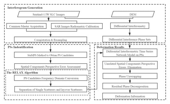
3.3.3. Part 3—The Spectral Analysis Method RELAX Combined with the PS-InSAR Technique

After the BF, SVD, and RELAX methods were compared through simulation experiments, the RELAX algorithm was utilized to convert the PSC in the frequency domain. By analyzing the peak characteristics of the scatterers in the elevation direction, the layover scatterers were identified, separated, and filtered. Finally, the PS-InSAR technique with the RELAX algorithm was applied to monitor the land subsidence over the study site. Based on the accurate leveling measurements, the land subsidence monitoring results were evaluated and analyzed to illustrate the effectiveness of the proposed PS-InSAR+RELAX method over the PS-InSAR technique.

4. Results

4.1. Model Simulations

As observed on the spectrum power graphs, similar trends were observed for all three spectral analysis methods (BF, SVD, and RELAX). There is one sharp distinct peak in the case of a single scatterer detected within one pixel for both baseline numbers 15 and 30 (Figure 4a,b, respectively). In the case of layover scatterers, however, two peaks are observed in both cases of baseline numbers 15 and 30 (Figure 5a,b). The trend strongly suggests that all three methods are capable of converting the scatterers to a frequency domain, and all can identify the single and double scatterer by the peak characteristics of the elevation direction.
Furthermore, for all three methods, the spectrum power is suppressed in the range of approximately 0~0.4, suggesting that the side-lobe effect generates the noise within this range. When the number of baselines changes from 15 to 30, BF produces the most noise, followed by SVD, and then by RELAX, which has the least amount of noise. When the spectrum power is in the range of 0.4~1, the peak position is close to the set scatterer height position at 40 m for all three methods. When the curve of the scatterer is 40 m, the peak positions are best defined for RELAX, then SVD, and BF.
The simulation results of layover scatterers show low spectrum power in the range of 0~0.4, because all three methods also generate noise due to the side-lobe effect. When the number of baselines changes from 15 to 30, the most elevated noise is observed for BF, followed by SVD, and then RELAX. When the spectrum power is in the range of 0.4~1, when all three methods have two sharp peaks, the positions of the peaks are close to the set scatterer height of 40 m and 80 m. At the height of the scatterers of 40 m and 80 m, the curves of the peaks are best defined (most pointed) for RELAX, then for SVD and BF.
The equivalent synthetic aperture in the NSR direction of SAR tomography is determined by the orthogonal baseline span. The NSR to Rayleigh resolution corresponding to the equivalent synthetic aperture is δ S (Equation (8)). With respect to the NSR resolutions, the results show that the NSR resolutions of BF and SVD are similar (Figure 6 and Figure 7). For both methods, the position of the scatterers can be identified when the NSR height of the two scatterers is greater than 24 m. Different from BF and SVD, the two scatterers can be identified at the lower NSR height of 14 m when RELAX is used, making this method more effective (Figure 8). These cutoff points of 24 m and 14 m suggest that the scatterers whose heights are below these values cannot be identified. The deviation of the scatterers at the given NSR positions are smaller than their actual position.

4.2. PS Identification

To demonstrate the effectiveness of RELAX in identifying and separating single and layover scatterers, the RELAX-derived scatterers are displayed over the experimental area B in Figure 9 (the yellow frame in Figure 2). While most of the single scatterers (red dots) are located in the lower part of buildings and along roads, the layover scatterers (blue dots) are commonly observed in the upper parts of the buildings. This is the expected interaction between buildings and the ground when the typical dihedral angle structure is formed.
The PS identification results based on the PSC obtained by StaMPS where RELAX has been used to separate and remove the layover scatterers are shown over the experimental area A in Figure 10. It can be observed that the results of the PS identification using PS-InSAR+RELAX and PS-InSAR techniques are relatively similar in spatial distribution. However, it is evident that the number and density of PSs identified by PS-InSAR+RELAX is reduced, suggesting that RELAX is advantageous in identifying, separating, and then filtering out the layover scatterers that appear due to the dense distribution of buildings. The number and density of PSs are reduced and visually simplified as the combined method PS-InSAR+RELAX can effectively reduce the influence of layover on PS identification.
The statistical parameters (intensity mean and intensity standard deviation) and the mean coherence coefficients are calculated and compared for the PS-InSAR+RELAX and PS-InSAR techniques in Table 3 and Figure 11. For the comparison to be valid, in both cases, the thresholds are set according to the same false alarm probability. The results show that the mean intensity of PSs identified by using PS-InSAR+RELAX and PS-InSAR are 68.42 and 14.62, respectively, and that the intensity standard deviations of the PSs identified by using PS-InSAR+RELAX and PS-InSAR techniques are 4.68 and 8.62, respectively. The considerably higher intensity mean and much lower intensity standard deviation demonstrate stronger and more stable scattering characteristics of the PS-InSAR+RELAX obtained PSs. At the same time, the density of PSs identified by PS-InSAR+RELAX reaches the value of 1725 PSs per square kilometer. According to [7], a density larger than 3 PSs per square kilometer must be reached to successfully monitor land subsidence.
The mean coherence coefficients of the PS identified by the PS-InSAR+RELAX and PS-InSAR techniques is shown in Figure 11. While the number of identified PSs is higher for PS-InSAR in the low-coherence range (0~0.6), the trend is changed in the range of high coherence (0.65~0.95) where the number of identified PSs increases for PS-InSAR+RELAX. Overall, the PSs identified by PS-InSAR+RELAX is more coherent than those identified by the PS-InSAR only technique.

4.3. Land Subsidence Monitoring and Validation

The overall spatial trends of the land subsidence rates generated using PS-InSAR+RELAX and PS-InSAR are roughly similar (Figure 12). Less subsidence was observed in the eastern region of the study area, while some major hotspots were observed in the western and southwestern regions. From 2014 to 2016, the land subsidence rates range between −110.4 mm/year and 5.5 mm/year. The area with the highest land subsidence rate was located in the Chaoyang district and at the border area between Chaoyang and Tongzhou. The land subsidence bowl includes the Chaoyang district, which is the economic center of Beijing, and the Tongzhou district, the sub-center of the city. Although the spatial trend of land subsidence was similarly distributed, less extensive land subsidence was observed for the PS-InSAR+RELAX technique. The extent of the land subsidence bowl appears to be smaller, as well as the hotspot area where land subsidence rate exceeded 110 mm/year.
The land subsidence information obtained by the PS-InSAR+RELAX and PS-InSAR techniques were validated against leveling measurements. Since the identified PSs were mainly located on buildings, and leveling benchmarks (BMs) in open land within a certain distance from the buildings, the PSs and benchmarks did not completely overlap in space [42]. Therefore, the Nearest Neighbor Index (NNI) method [43], were used to extract the average land subsidence rates of PSs that are within 200 m from the BM locations, which were then compared with leveling measurements of each BM. The differences between the PS-InSAR obtained and leveling measurements ranged from 2.37 to 9.32 mm/year, with the mean and standard deviation of 5.41 mm/year and 2.11 mm/year, respectively (Table 4). Considerably lower differences were observed between the PS-InSAR+RELAX obtained estimations and leveling measurements. The differences ranged from 1.28 to 3.95 mm/year, and their mean and standard deviation were 2.12 mm/year and 0.75 mm/year, respectively (Table 5). Compared with PS-InSAR+RELAX, PS-InSAR not only has a maximum monitoring error of 9.32 mm/year, but its mean and standard deviation of land subsidence monitoring error is about twice that of PS-InSAR+RELAX.
Furthermore, the correlation coefficients (r) between the leveling measurements and land subsidence rate estimations are r = 0.95 (Figure 13) and r = 0.98 (Figure 14) for PS-InSAR and PS-InSAR+RELAX, respectively. Overall, the results show the better performance of the PS-InSAR+RELAX technique. By reducing the impact of the layover effect on the PS identification accuracy, this combined method improved the urban land subsidence monitoring over the study site.

5. Discussion

As the side-looking geometry of SAR causes the feature displacement and layover effect that depends on the height of the features, SAR image interpretation is particularly challenging over dense urban areas with high-rise buildings [36]. The layover scatterers do not have amplitude stability and spatial coherence, and as such they hinder PS identification, which is a critical processing step for the monitoring of land subsidence. To overcome these limitations, commonly observed within the PS-InSAR technique, it is necessary to improve the process of PS identification.
In this study, we have demonstrated that the proposed spectral analysis method called RELAX is advantageous over some other spectral analysis methods, such as the BF and SVD tomography imaging methods, in identifying single and layover scatterers. For that reason, the integrated PS-InSAR+RELAX technique is advantageous over the PS-InSAR technique in identifying PSs, and consequently, in monitoring land subsidence. The results demonstrate the better capability of RELAX to identity layover scatterers with more accuracy than BF and SVD (Figure 4, Figure 5, Figure 6, Figure 7 and Figure 8), and to identify PSs with higher coherency and intensity (Table 3). It is the number and density of PSs that further improved the land subsidence monitoring in the study area (Figure 9, Figure 10 and Figure 11).
As PS-InSAR technique is a very mature technique, the monitored land subsidence has good accuracy. Although both methods, PS-InSAR and PS-InSAR+RELAX, appear as being similarly reliable in this study, over the whole study area, there are obvious differences in the extent and intensity of the land subsidence bowl, which is visibly reduced in the case of PS-InSAR+RELAX (Figure 12, Table 4 and Table 5). The better agreement between the PS-InSAR+RELAX derived estimates and the leveling measurements (Figure 13 and Figure 14), it confirms that the PS-InSAR techniques overestimated the land subsidence rate in the study area. The overestimated results on monitoring land subsidence in the Beijing region are similar to Yun’s find [44].
Our findings are considered helpful, as they concern an urban area that has one of the largest segments of Beijing’s population and is a powerful economic center of Beijing. Many high-rise buildings are concentrated in the CBD, and the mean annual subsidence of more than 100 mm/year cannot be neglected. Even minor over- or under-estimations of land subsidence can be critical for millions of people’s property and life safety. Overall, the constant improvement of the InSAR technique is required to better understand the phenomenon of land subsidence. Refinements of estimated layover scatterers in high-rise dense urban areas is an ongoing challenge for accurate land subsidence calculations. In our future work, we will attempt to add other indicators to evaluate the quality of PSs to illustrate the reliability of the identified PSs more fully.

6. Conclusions

Owing to the layover effect within the PS-InSAR techniques, PS identification is a challenge in monitoring land subsidence, especially in dense urban areas with high-rise buildings. In recent years, several spectral analysis methods were found to be useful in identifying single and layover scatterers, which improved PSs identification and ultimately land surface monitoring. Out of three spectral analysis methods (BF, SVD, and RELAX), whose performance was compared in the present study to identify layover scatterers, RELAX was demonstrated to be the most reliable algorithm. Its advantageous performance was examined from the aspects of the number of baselines and the NSR resolution. RELAX was then coupled with the PS-InSAR technique (PS-InSAR+RELAX) to improve the identification of PSs. Within this method, PSs were converted into the frequency domain and based on the peaks of reconstructed scatterers’ elevation range, the frequency domain characteristics of both single and layover scatterers were obtained, and PSs identified. The results cast new light on PS identification techniques and on the PS-InSAR technique needed to study land subsidence. The proposed method was applied to a time series Sentinel-1A imagery acquired over the study area situated in the Beijing Plain, where urban land subsidence is recognized as a continuous safety problem. The final results demonstrated the advantageous performance of the integrated PS-InSAR+RELAX over the PS-InSAR technique, which was found to overestimate the land subsidence in the study area. The land subsidence rate obtained with PS-InSAR+RELAX agreed well with the leveling measurements obtained. The present study and its findings have important implications for the safety of the population in the Beijing Plain region.

Author Contributions

D.Z. performed the simulations, analyzed the data, and prepared the manuscript with contributions from all co-authors. A.S.-M. made important suggestions and revised the manuscript. J.Y. provided crucial guidance and support through the research. L.Z. and B.C. contributed significantly and provided funding. N.M. made helpful suggestions for data processing. All authors have read and agreed to the published version of the manuscript.

Funding

This research was funded by the National Natural Science Foundation of China (grant number 41671417) and the Beijing Outstanding Young Scientist Program (BJJWZYJH01201910028032) and Capacity Building for Sci-Tech Innovation Fundamental Scientific Research Funds (01119530050175) and Beijing Natural Science (grant number 8202008).

Conflicts of Interest

The authors declare no conflict of interest.

References

  1. Chaussard, E.; Wdowinski, S.; Cabral-Cano, E.; Amelung, F. Land subsidence in central Mexico detected by ALOS InSAR time-series. Remote Sens. Environ. 2014, 140, 94–106. [Google Scholar] [CrossRef]
  2. Lin, H.; Ma, P.F.; Wang, W.X. Urban Infrastructure Health Monitoring with Spaceborne Multi-temporal Synthetic Aperture Radar Interferometry. Acta Geod. Cartogr. Sin. 2017, 46, 1421–1433. [Google Scholar] [CrossRef]
  3. Hooper, A.; Zebker, H.A. Phase unwrapping in three dimensions with application to InSAR time series. JOSAA 2007, 24, 2737–2747. [Google Scholar] [CrossRef] [Green Version]
  4. Crosetto, M.; Monserrat, O.; Cuevas-Gonzalez, M. Persistent Scatterer Interferometry: A review. ISPSR J. Photogramm. Remote Sens. 2016, 115, 78–89. [Google Scholar] [CrossRef] [Green Version]
  5. Ferretti, A.; Prati, C.; Rocca, F. Permanent scatterers in SAR interferometry. IEEE Trans. Geosci. Remote Sens. 2001, 39, 8–20. [Google Scholar] [CrossRef]
  6. Hooper, A.; Zebker, H.; Segall, P. A new Method for Measuring Deformation on Volcanoes and Other Natural Terrains Deformation Using InSAR Persistent Scatterers. Geophys. Res. Lett. 2004, 31, 1–5. [Google Scholar] [CrossRef]
  7. Ferretti, A.; Prati, C.; Rocca, F. Nonlinear Subsidence Rate Estimation Using Permanent Scatterers in Differential SAR Interferometry. IEEE Trans. Geosci. Remote Sens. 2002, 38, 2202–2212. [Google Scholar] [CrossRef] [Green Version]
  8. Mora, O.; Mallorqui, J.J.; Duro, J. Linear and nonlinear terrain deformation maps from a reduced set of interferometric SAR images. IEEE Trans. Geosci. Remote Sens. 2003, 41, 2243–2253. [Google Scholar] [CrossRef]
  9. Berardino, P.; Fornaro, G.; Lanari, R.; Sansosti, E. A new algorithm for surface deformation monitoring based on small baseline differential SAR interferograms. IEEE Trans. Geosci. Remote Sens. 2002, 40, 2375–2383. [Google Scholar] [CrossRef] [Green Version]
  10. Ferretti, A.; Fumagalli, A.; Novali, F.; Prati, C.; Rocca, F.; Rucci, A. A newalgorithm for processing interferometric data-stacks: SqueeSAR. IEEE Trans. Geosci. Remote Sens. 2011, 49, 3460–3470. [Google Scholar] [CrossRef]
  11. Goel, K.; Adam, N. A distributed scatterer interferometry approach for precision monitoring of known surface deformation phenomena. IEEE Trans. Geosci. Remote Sens. 2014, 52, 5454–5468. [Google Scholar] [CrossRef]
  12. Devanthéry, N.; Crosetto, M.; Monserrat, O.; Cuevas-González, M.; Crippa, B. An approach to persistent scatterer interferometry. Remote Sens. 2014, 6, 6662–6679. [Google Scholar] [CrossRef] [Green Version]
  13. Confuorto, P.; Martire, D.D.; Centolanza, G.; Iglesias, R.; Mallorqui, J.J.; Novellino, A.; Plank, S.; Ramondini, M.; Thuro, K.; Calcaterra, D. Post-failure evolution analysis of a rainfall-triggered landslide by multi-temporal interferometry SAR approaches integrated with geotechnical analysis. Remote Sens. Environ. 2017, 188, 51–72. [Google Scholar] [CrossRef]
  14. Iglesias, R.; Mallorqui, J.J.; Monells, D.; López-Martínez, C.; Fabregas, X.; Aguasca, A.; Gili, J.A.; Corominas, J. PSI Deformation Map Retrieval by Means of Temporal Sublook Coherence on Reduced Sets of SAR Images. Remote Sens. 2015, 7, 530–563. [Google Scholar] [CrossRef] [Green Version]
  15. Liao, M.S.; Wei, L.H.; Wang, Z.Y.; Balz, T.; Zhang, L. Compressive Sensing in High-resolution 3D SAR Tomography of Urban Scenarios. J. Radars 2015, 4, 123–129. [Google Scholar] [CrossRef]
  16. Fornaro, G.; Lombardini, F.; Pauciullo, A.; Reale, D.; Viviani, F. Tomographic Processing of Interferometric SAR Data: Developments, applications, and future research perspectives. IEEE Signal Process. Mag. 2014, 31, 41–50. [Google Scholar] [CrossRef]
  17. Chen, F.L.; Wu, Y.H.; Zhang, Y.M. Motion and Structural Instability Monitoring of Ming Dynasty City Walls by Two-Step Tomo-PSInSAR Approach in Nanjing City, China. Remote Sens. 2017, 9, 371. [Google Scholar] [CrossRef] [Green Version]
  18. Ma, P.F.; Liu, Y.Z.; Wang, W.X.; Lin, L. Optimization of PSInSAR networks with application to TomoSAR for full detection of single and double persistent scatterers. Remote Sens. Lett. 2019, 10, 717–725. [Google Scholar] [CrossRef]
  19. De, M.A.; Fornaro, G.; Pauciullo, A. Detection of single scatterers in multidimensional SAR imaging. IEEE Trans. Geosci. Remote Sens. 2009, 47, 2284–2297. [Google Scholar] [CrossRef]
  20. Zhang, M.; Burbey, T.J. Inverse modeling using PS-InSAR data for improved land subsidence simulation in Las Vegas Valley, Nevada. Hydrol. Process 2016. [Google Scholar] [CrossRef]
  21. Fornaro, G.; Serafino, F.; Soldovieri, F. Three–Dimensional Focusing with Multipass SAR Data. IEEE Trans. Geosci. Remote Sens. 2003, 41, 507–517. [Google Scholar] [CrossRef]
  22. Fornaro, G.; Serafino, F. Imaging of Single and Double Scatterers in Urban Areas via SAR Tomography. IEEE Trans. Geosci. Remote Sens. 2006, 44, 3497–3505. [Google Scholar] [CrossRef]
  23. Ren, X.Z.; Yang, R.L. Improved RELAX Algorithm for SAR Tomography. J. Data Acquis. Proc. 2010, 25, 302–306. [Google Scholar] [CrossRef]
  24. Stoica, P.; Nehorai, A. Performance study of conditional and unconditional direction-of-arrival estimation. IEEE Trans. Acoust. Speech. Signal Proc. 1990, 38, 1783–1795. [Google Scholar] [CrossRef]
  25. Fornaro, G.; Serafino, F.; Lombardini, F. Three-dimensional multipass SAR focusing: Experiments with long-term spaceborne data. IEEE Trans. Geosci. Remote Sens. 2005, 43, 702–712. [Google Scholar] [CrossRef]
  26. Fornaro, G.; Monti, G.A. Joint multibaseline SAR interferometry. EURASIP J. Appl. Signal Process. 2005, 20, 3194–3205. [Google Scholar] [CrossRef] [Green Version]
  27. Li, J.; Stoica, P.; Zheng, D. An Efficient Algorithm for Two-dimensional Frequency Estimation. Multidimens. Syst. Signal Proc. 1996, 7, 151–178. [Google Scholar] [CrossRef]
  28. Pauciullo, A.; Reale, D.; De, M.A. Detection of Double Scatterers in SAR Tomography. IEEE Trans. Geosci. Remote Sens. 2012, 50, 3567–3586. [Google Scholar] [CrossRef]
  29. Budillon, A.; Schirinzi, G. GLRT Based on Support Estimation for Multiple Scatterers Detection in SAR Tomography. IEEE J. Appl. Earth Observ. Remote Sens. 2016, 9, 1086–1094. [Google Scholar] [CrossRef]
  30. Dănișor, C.; Fornaro, G.; Pauciullo, A. Super-Resolution Multi-Look Detection in SAR Tomography. Remote Sens. 2018, 10, 1894. [Google Scholar] [CrossRef] [Green Version]
  31. Zhou, C.D.; Gong, H.L.; Zhang, Y.Q.; Warner, T.; Wang, C. Spatiotemporal Evolution of Land Subsidence in the Beijing Plain 2003–2015 Using Persistent Scatterer Interferometry (PSI) with Multi-Source SAR Data. Remote Sens. 2018, 10, 552. [Google Scholar] [CrossRef] [Green Version]
  32. Zhang, Y.H.; Wu, H.A.; Kang, Y.H.; Zhu, C.G. Ground Subsidence in the Beijing-Tianjin-Hebei Region from 1992 to2014 Revealed by Multiple SAR Stacks. Remote Sens. 2016, 8, 675. [Google Scholar] [CrossRef] [Green Version]
  33. Holzner, J.; Bamler, R. Burst-Mode and ScanSAR Interferometry. IEEE Trans. Geosci. Remote Sens. 2002, 40, 1917–1934. [Google Scholar] [CrossRef] [Green Version]
  34. González, P.J.; Bagnardi, M.; Hooper, A.J. The 2014-2015 eruption of Fogo volcano: Geodetic modeling of Sentinel-1 TOPS interferometry. Geophys. Res. Lett. 2015, 42, 9239–9246. [Google Scholar] [CrossRef] [Green Version]
  35. Shang, D. WorldView-2 high-resolution satellite successfully launched. Remote Sens. Land Res. 2009, 4, 109. [Google Scholar]
  36. Lin, H.; Ma, P.F.; Lan, H.X. Basic Principles, Key Techniques and Applications of Tomographic SAR Imaging. J. Geomatics. 2015, 40, 1–6. [Google Scholar] [CrossRef]
  37. Sandwell, D.; Mellors, R.; Tong, X.; Wei, M.; Wessel, P. Open Radar Interferometry Software for Mapping Surface Deformation. Eos Trans. AGU 2011, 92, 234. [Google Scholar] [CrossRef] [Green Version]
  38. Farr, T.; Rosen, P.; Caro, E.; Crippen, R.; Duren, R.; Hensley, S.; Alsdorf, D. The shuttle radar topography mission. Rev. Geophys. 2007, 45. [Google Scholar] [CrossRef] [Green Version]
  39. Hooper, A.; Bekaert, D.; Spaans, K.; Arıkan, M. Recent advances in SAR interferometry time series analysis for measuring crustal deformation. Tectonophysics 2011, 514, 1–13. [Google Scholar] [CrossRef]
  40. Bekaert, D.P.S.; Walters, R.J.; Wright, T.J.; Hooper, A.J.; Parker, D.J. Statistical comparison of InSAR tropospheric correction techniques. Remote Sens. Environ. 2015, 170, 40–47. [Google Scholar] [CrossRef] [Green Version]
  41. Dee, D.P.; Uppala, S.M.; Simmons, A.J.; Berrisford, P.; Poli, P.; Kobayashi, S.; Andrea, U. The ERA-Interim reanalysis: Configuration and performance of the data assimilation system. Q. J. R. Meteorol. Soc. 2011, 137, 553–597. [Google Scholar] [CrossRef]
  42. Wang, B.C.; Yuan, S.L.; Wang, J.H.; Guo, L.F. Accuracy Analysis and Evaluation of InSAR Land Subsidence Monitoring. Remote Sens. Inf. 2015, 30, 8–13. [Google Scholar] [CrossRef]
  43. Yuan, Y.; Zhou, C.; Qin, B. A Nearest Neighbor Index Clustering Algorithm for Ecological Regionalization Based on Multi-layer Grid Model. Geo-Inf. Sci. 2011, 13, 1–11. [Google Scholar] [CrossRef]
  44. Yun, Y.; Lü, X.L.; Fu, X.K. Application of spaceborne interferometric synthetic aperture radar to geohazard monitoring. J. Radars 2020, 9, 73–85. [Google Scholar] [CrossRef]
Figure 1. The geographical location of the study area. The blue box represents the range of study areas. The red box represents the experimental area A in Chaoyang CBD. The yellow box indicates the locations of the experimental area B with dense buildings in Chaoyang CBD. The black triangles are the position of the benchmarks.
Remotesensing 12 02730 g001
Figure 2. Baseline configurations of single-master Interferograms. The red dot indicates the master image used as a reference for each track. The blue dots represent the slave images. The blue lines connect the pairs (Interferograms).
Remotesensing 12 02730 g002
Figure 3. Workflow of the joint method PS-InSAR+RELAX technique used for land subsidence monitoring.
Remotesensing 12 02730 g003
Figure 4. Simulation results of single scatterers under different numbers of baselines. Hs is 40 m; the baseline numbers of (a) and (b) are 15 and 30, respectively.
Remotesensing 12 02730 g004
Figure 5. Simulation results of layover scatterers under different numbers of baselines. Hs is 40 m and 80 m, the baseline numbers of (a) and (b) are 15 and 30 respectively.
Remotesensing 12 02730 g005
Figure 6. Simulation results of NSR resolution for BF.
Remotesensing 12 02730 g006
Figure 7. Simulation results of NSR resolution for SVD.
Remotesensing 12 02730 g007
Figure 8. Simulation results of NSR resolution for RELAX.
Remotesensing 12 02730 g008
Figure 9. RELAX-derived single (red dots) and layover (blue dots) scatterers displayed over the experimental area B with highly dense urban setting (see Figure 1).
Remotesensing 12 02730 g009
Figure 10. The identified PSs using (a) PS-InSAR technique and (b) PS-InSAR+RELAX in the experimental area A in Chaoyang CBD. The blue dots indicate the persistent scatterers displayed over the WorldView-2 image.
Remotesensing 12 02730 g010
Figure 11. PS coherence coefficients for PS-InSAR and PS-InSAR+RELAX.
Remotesensing 12 02730 g011
Figure 12. Comparison of land subsidence rate calculated for the study area for the period between 2014 and 2016, using (a) PS-InSAR and (b) PS-InSAR+RELAX. Positive land subsidence rates (cold colors) represent the motion of the ground toward the satellite, and negative land subsidence rates (warm colors) represent the motion away from the satellite.
Remotesensing 12 02730 g012
Figure 13. Comparisons of PS-InSAR technique obtained land subsidence rates and leveling measurement rates from 2014 to 2016. The location of benchmarks is marked as “BM1-BM9” (see Figure 2).
Remotesensing 12 02730 g013
Figure 14. Comparisons of PS-InSAR+RELAX obtained land subsidence rates and leveling measurement rates from 2014 to 2016. The location of benchmarks is marked as “BM1-BM9” (see Figure 2).
Remotesensing 12 02730 g014
Table 1. The parameters of the Sentinel-1A SAR data (ESA, 2013).
ParameterValue
Wavelength5.6 cm
Incidence Angle39.6°
Orbital Height693 km
PolarizationsHH + HV, VH + VV, HH, VV
Spatial Resolution20 m (ground range) × 5 m (azimuth)
Pixel Spacing2.3 m (slant range) × 13.9 m (azimuth)
Table 2. Simulation experiment parameter setting.
ParameterValue
Wavelength ( λ )5.6 cm
Average Satellite Height (H)690 km
Average Distance (Rg)690 km
Total Perpendicular baseline Length (Bv)300 m
Number of Flights (N)31
Table 3. Statistical overview of the PS identification using PS-InSAR+RELAX and PS-InSAR techniques.
MethodsThe Number of PSThe Density of PS/km2Intensity MeanIntensity Standard Deviation
PS-InSAR16352187614.628.62
PS-InSAR+RELAX14258172568.424.68
Table 4. Comparison of land subsidence results by PS-InSAR technique with leveling measurement (mm/year).
Benchmarks NumberLeveling MeasurementPS-InSARDifference
BM1−109.15−116.577.42
BM2−106.26−115.589.32
BM3−63.32−70.316.99
BM447.76−53.355.59
BM510.577.293.28
BM612.129.752.37
BM79.345.983.36
BM812.256.965.29
BM910.695.645.05
Mean
Standard deviation
5.41
2.11
Table 5. Comparison of land subsidence results by PS-InSAR+RELAX with leveling measurement (mm/year).
Benchmarks NumberLeveling MeasurementPS-InSAR+RELAXDifference
BM1−109.15−110.431.28
BM2−106.26−110.213.95
BM3−63.32−65.692.37
BM447.76−50.212.45
BM510.578.591.98
BM612.1210.671.45
BM79.347.152.19
BM812.2510.671.58
BM910.698.861.83
Mean
Standard deviation
2.12
0.75

