Spatiotemporal Variation of Surface Urban Heat Islands in Relation to Land Cover Composition and Configuration: A Multi-Scale Case Study of Xi’an, China

Abstract

Urban heat islands (UHI) can lead to multiple adverse impacts, including increased air pollution, morbidity, and energy consumption. The association between UHI effects and land cover characteristics has been extensively studied but is insufficiently understood in inland cities due to their unique urban environments. This study sought to investigate the spatiotemporal variations of the thermal environment and their relationships with land cover composition and configuration in Xi’an, the largest city in northwestern China. Land cover maps were classified and land surface temperature (LST) was estimated using Landsat imagery in six time periods from 1995 to 2020. The variations of surface heat island were captured using multi-temporal LST data and a surface urban heat island intensity (SUHII) indicator. The relationship between land cover features and land surface temperature was analyzed through multi-resolution grids and correlation analysis. The results showed that mean SUHII in the study area increased from 0.683 °C in 1995 to 2.759 °C in 2020. The densities of impervious surfaces had a stronger impact on LST than green space, with Pearson’s correlation coefficient r ranging from 0.59 to 0.97. The correlation between normalized difference impervious surface index and LST was enhanced with the enlargement of the grid cell size. The correlations between normalized difference vegetation index and LST reached maxima and stabilized at grid cell sizes of 210 and 240 m. Increasing the total area and aggregation level of urban green space alleviated the negative impacts of UHI in the study area. Our results also highlight the necessity of multi-scale analysis for examining the relationships between landscape configuration metrics and LST. These findings improved our understanding of the spatiotemporal variation of the surface urban heat island effect and its relationship with land cover features in a major inland city of China.

1. Introduction

The proportion of urban population globally is about 55%. It is projected to continue to increase, and nearly 90% of the growth will occur in Asia and Africa [1]. The urbanization process worldwide has caused the alteration of land cover and land use and a series of environmental problems [2]. Among them, a well-known phenomenon is the urban heat island (UHI), in which the temperature in urban areas is significantly higher than nearby rural areas. UHIs can lead to multiple consequences, such as increased air pollution, morbidity, and energy consumption, and thus, have an adverse impact on residents’ lives in cities and towns [3]. In particular, the consequences of the UHI effect is expected to be aggravated by global warming and an increasingly urbanizing world [4]. Therefore, the UHI effect has been widely investigated from local to global scales.

The UHI phenomenon can be characterized in two methods: atmospheric UHI and surface UHI. Atmospheric UHI is measured by meteorological stations or via field surveys using equipment mounted on a car, balloon, or aircraft. Surface urban heat island (SUHI) documents the difference in land surface temperatures in cities and nearby rural areas observed by satellite sensors. Due to their repeatable, large-scale observations of Earth’s surface, satellites provide a superior data source for land surface temperature (LST) estimation and urban thermal environment characterization [5,6]. Thermal infrared bands of satellite sensors, such as AVHRR, MODIS, Landsat TM/ETM+/TIRS, and ASTER, have been used for LST retrieval and UHI measurement at various spatial and temporal scales [7,8,9,10]. Among them, Landsat satellites provide long, continuous observation of land surface and have been widely used to explore the spatiotemporal evolution of urban thermal environment [11,12].

A variety of indicators have been developed to quantify the spatial pattern and temporal variation of SUHI using land surface temperature. The LST difference between urban and rural areas was a fundamental indicator to identify SUHI variations [5]. One limitation of the urban–rural difference indicator is that the distinction between urban and rural remains confusing and there lacks a standardized method to define urban and rural extents [13,14]. Several other indicators such as the urban–agriculture difference, urban–water difference, Gaussian magnitude, and hot island area were also developed to measure the magnitude of SUHI [15]. To provide an objective protocol for measuring the magnitude of the urban heat island effect, the concept of Local Climate Zones (LCZ) was proposed [16,17]. Under this framework, UHI magnitude is defined as the temperature difference between built-type and natural-type LCZ classes [18,19].

Previous UHI studies have mainly concentrated on big and/or coastal cities where UHI effects are prominent. Imhoff et al. [20] found that the amplitude of UHI is seasonally asymmetric with higher temperature differences in summer than in winter, when controlling for ecological settings, across the 38 most populated urban areas in the conterminous United States. Peng et al. [21] reported that the daytime intensity of SUHI was significantly higher than nighttime across more than 400 big cities globally and that the spatial distribution of SUHI corelates with the differences in vegetation cover between urban and suburban areas. Zhou et al. [22] analyzed SUHI in 32 major cities in China and attributed their spatial variations to such driving forces as vegetation, anthropogenic heat release, climate, and built-up area density. Firozjaei et al. [23] conducted a comparative analysis of surface anthropogenic heat islands across six megacities with varying geographic and climate settings. By comparing the UHI in different cities, these studies revealed the large spatial, diurnal, and seasonal heterogeneity in SUHI across cities due to their different driving variables.

Since land cover characteristics and their changes are closely related to the distribution of land surface temperature, their relationship has been investigated in numerous studies. Landscape composition is the amount of land cover categories within a defined spatial unit. The influences of landscape composition on urban LST were well documented [24,25]. Gogoi et al. found that 25% to 50% of observed overall warming was associated land use and land cover changes over eastern India [26]. Guha et al. analyzed seasonal variability in land surface temperature and their relationship with spectral indices such as normalized difference vegetation index (NDVI) and normalized difference built-up index (NDBI) in Raipur [27]. Logan et al. examined the influence of urban characteristics such as building floor area, NDBI, and NDVI on land surface temperature in four cities across the United States [28]. Using Landsat 8 satellite imagery, Song et al. quantified the effects of building density on land surface temperature across 21 cities in China [29]. Landscape configuration metrics quantify the spatial characteristics or arrangement of land cover patches. Using these metrics, the influences of size, shape, and segmentation of land cover on LST have been analyzed [30,31]. Xie et al. used structural equation models to describe the relationship between land scape indicators such as patch density, largest patch index, aggregation index, and surface temperature [32]. Despite these efforts, the relationship between the UHI and land cover composition and spatial arrangement are not fully understood due to the heterogeneity of urban environments. Previous reported conflict associations between land cover patterns and LST in case studies of different cities [33,34]. They also revealed that the relationship between landscape composition and LST was scale-dependent [35,36,37]. Multi-scale analysis has been necessary to understand the scale-dependent effect of UHI in ecological studies [38,39].

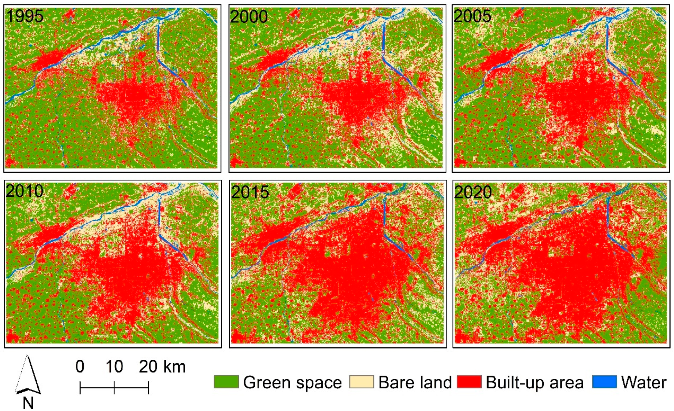
This study takes Xi’an, China, as the study area to analyze the spatiotemporal variations of the thermal environment and their relationships with land cover characteristics using remote sensing data. The relationship between the amount and arrangement of urban green space and impervious surfaces and LST was explored using a multi-scale analysis approach. This study will enhance our understanding of the spatiotemporal variation of SUHI effect and its association with land cover features in an inland city.

2. Materials

2.1. Study Area

Xi’an, the largest city in northwestern China, consists of 11 municipal districts and 2 counties. With a total area of 10,752 km², the population in Xi’an reached 10 million in 2018, of which about 75% were urban residents. It has a temperate continental monsoon climate. Winters are dry and cold and summers are rainy and hot. The mean temperature ranges from 26.3 to 26.6 °C in July, and −1.2 to 0.0 °C in January [40].

As the administrative, economic, and cultural center of Shaanxi Province, Xi’an has been one of the fastest urbanizing cities in China. In particular, the China Western Development national strategy has greatly promoted its economic growth since 2000. The rapid urban growth in Xi’an caused a decrease in forest areas, an increase in air pollution, and a degradation of environmental quality [41]. To investigate the spatial and temporal variation of thermal environment in metropolitan areas, the six municipal districts of Xi’an were selected as our study area, including Weiyang, Baqiao, Lianhu, Xincheng, Beilin, Yanta, and their surrounding areas (Figure 1).

2.2. Satellite Data

Six Landsat images acquired in 1995, 2000, 2004, 2011, 2014, and 2020 were used to depict the land cover and thermal environment in the study area with a five-year interval since 1995 (

Table 1. Landsat images used.

Satellite and Sensor	Spatial Resolution (m)		Local Overpass Time
	Multispectral	Thermal
Landsat5 TM	30	120	19950507 10:55:37 (Day)
Landsat5 TM	30	120	20000520 10:55:37 (Day)
Landsat7 ETM+	30	60	20040421 11:08:56 (Day)
Landsat5 TM	30	120	20100430 11:10:38 (Day)
Landsat8 OLI	30	100	20140511 11:19:25 (Day)
Landsat8 OLI	30	100	20200409 11:19:28 (Day)

). Since climate conditions such as air temperature, humidity, and cloudiness vary least in spring in the study area, satellite images in April and May under clear sky conditions were selected for each year to reduce the variation of the atmospheric background [42]. The images were acquired by Landsat 5 TM, Landsat 7 ETM+, and Landsat 8 OLI/TIRS, respectively. The Level-1 Landsat products (L1TP) were obtained from the USGS Earth Explorer (https://earthexplorer.usgs.gov/). Atmospheric correction was conducted on the Landsat data by using the FLAASH module in ENVI 5.3 software.

Due to a malfunction of the Scan Line Corrector, Landsat 7 ETM+ imagery acquired after May 2003 was flawed. In each image scene, about 20% of pixels were lost. We filled the gaps in the Landsat 7 ETM+ image in 2004 using the Landsat Gapfill tool in the ENVI software.

3. Methods

3.1. Land Cover Classification

A random forest classifier was implemented to obtain the land cover maps in the study area. Land cover types in the classification included built-up area, bare land, green space, and water. In addition to original data, normalized difference impervious surface index (NDISI) [43], normalized difference vegetation index (NDVI) [44], and normalized water index (NDWI) [45] were derived as additional input features for the classification.

$$NDVI=\frac{NIR-Red}{NIR+Red}$$

(1)

$$MNDWI=\frac{Green-MIR}{Green+MIR}$$

(2)

$$NDISI=\frac{TIRS-\left(MNDWI+NIR+MIR\right)/3}{TIRS+\left(MNDWI+NIR+MIR\right)/3}$$

(3)

Afterward, post-classification correction was performed manually to further improve the classification results. Following the “good practice” recommendations for accuracy assessment, a stratified random sampling method with mapped classes as strata was implemented to assess the overall accuracy of classified land cover maps quantitively [46,47]. To obtain a target standard error for overall accuracy of 0.01, the sample sizes range approximately from 500 (user’s accuracy 95%) to 900 (user’s accuracy 90%) [48]. A minimum of 50 samples per land cover category is also desirable to ensure a sufficient representation of rare classes [48]. Hence, a total of 700 random sample points were collected as the validation dataset for each Landsat scene [49]. Among the sample points, 300 were assigned to built-up area, 150 to bare land, 200 to green space, and 50 to water. Reference ground truth information was collected from high resolution satellite images of Google Earth and the pan-sharpened images of the Landsat data.

Two metrics, the annual change area (ACA, km²) and annual rate of change (ACR, %), were used to measure the amount and rate of land cover change for each land cover category. The ACA and ACR are defined as follows:

$$ACA=\left(A_{end}-A_{start}\right)/d,$$

(4)

$$ACR=({\left(\frac{A_{end}}{A_{start}}\right)}^{1/d}-1)\times 100\%,$$

(5)

where $A_{start}$ and $A_{end}$ represent the areas of an individual land cover type at the start and end time point, respectively, and d is the time period from the start to the end time point. The ACA and ACR were calculated for each land cover type from 1995 to 2020 using the derived multi-temporal land cover maps.

3.2. Land Surface Temperature Retrieval

The digital numbers of the thermal bands from the original Landsat data (Band 6 in Landsat TM and ETM+, and Band 10 in Landsat TIRS) were converted to absolute radiance values. Then, the radiance values were converted to at-satellite brightness temperature in degrees Kelvin. Finally, the land surface temperature was calculated using:

$$LST=\frac{T_B}{1+\left(\lambda \times \frac{T_B}{\rho }\right)\ln \epsilon },$$

(6)

where $T_B$ is brightness temperature of the thermal bands; λ is wavelength of emitted radiance (λ = 11.457, 11.270, and 10.904 for Landsat TM, ETM+, and TIRS B10, respectively); ρ = h × c/σ, 1.438 × 10⁻² mk, where σ is Boltzmann constant, h is Planck’s radiation constant, c is velocity of light, and ε is the land surface emissivity [50].

By considering an image pixel as a mixture of bare soil and vegetation, land surface emissivity at the pixel level can be modeled using vegetation proportion and emissivities of vegetation of soil [50]. Land surface emissivity ε can be obtained from NDVI using a NDVI threshold method [51]. In this study, the land surface emissivity ε was estimated using a simplified equation [52]:

$$\epsilon =m{P}_v+n,$$

(7)

where $P_v$ is the vegetation coverage. By using typical constant values for the emissivities of vegetation and soil, m and n were calculated as 0.004 and 0.986, respectively [52].

The NDVI was derived using the red and near-infrared bands of Landsat data. Using NDVI data, vegetation coverage $P_v$ was derived using the following equation:

$$P_v={\left(\frac{NDVI-NDV{I}_{min}}{NDV{I}_{max}-NDV{I}_{min}}\right)}^2,$$

(8)

where $NDV{I}_{max}$ and $NDV{I}_{min}$ are the maximum and minimum vegetation index in the study area, respectively.

Due to the atmospheric background differences among satellite image scenes, LST cannot be used directly to compare UHI in the study area. To reduce the differences in the atmospheric background among the Landsat scenes, a normalization procedure was performed to rescale the LST to a range between 0 and 1 using the following equation [53]:

$$NLS{T}_i=\frac{LS{T}_i-LS{T}_{min}}{LS{T}_{max}-LS{T}_{min}},$$

(9)

where $NLS{T}_i$ refers to the normalized land surface temperature at pixel i, $LS{T}_i$ is the land surface temperature at pixel i, and $LS{T}_{min}$ and $LS{T}_{max}$ refer to the minimum and maximum LST in the study area, respectively. To remove the impacts of outliers, we chose the 5th and 95th percentile of each LST dataset as the maximum and minimum land surface temperature values. Due to the variation of LST during the study period, the maximum and minimum values of LST were calculated for each Landsat image.

3.3. Surface Urban Heat Island Intensity

Following the LCZ concept, the surface UHI intensity was defined as the land surface temperature difference between built-up and green space areas in this study [19,54]. At each built-up area pixel, the SUHII was calculated using the following formula:

$$SUHI{I}_i=T_{bui}-{\overline{T}}_{gs},$$

(10)

where $T_{bui}$ is land surface temperature at pixel i and ${\overline{T}}_{gs}$ is mean land surface temperature of green space pixels. The SUHII of the study area were further derived as:

$$SUHII=\frac{1}{n}{\sum }_{i=1}^{n}SUHI{I}_i,$$

(11)

where $SUHI{I}_i$ is the surface urban heat island at pixel i and n is the total number of built-up area pixels.

3.4. Landscape Analysis

3.4.1. Land cover composition analysis

In this study, the densities of green space and built-up area were used as landscape composition metrics. The influence of the density of impervious surfaces and green space on LST was examined based on grids at different spatial scales. Using the fishnet tool, we created square grids with cells of 30, 180, 270, 360, and 450m covering the entire study area [34]. The average values of LST, NDVI, and NDISI were calculated in each fishnet grid. Grid units that contained water pixels were excluded in the analysis.

3.4.2. Land Cover Configuration Analysis

The main characteristics describing the spatial pattern of land cover, including edge density, fragmentation, and the abundance, size, and shape of patches, can be represented by several spatial configuration landscape metrics [55]. As the basic elements that make up a landscape, patches represent relatively discrete areas of relatively homogeneous land cover types where patch boundaries are distinguished by discontinuities from their surroundings. A landscape contains a hierarchy of patch mosaics across a range of scales. Considering their potential effects on LST, interpretability, and redundancy, six landscape metrics were selected in our study (

Table 2. Description of landscape metrics [55].

Landscape Metrics	Abbreviation	Formula	Description
Percentage of landscape	PLAND	$\frac{{\sum }_{j=1}^n{a}_j}{A}\ast 100(\%)$	$a_j$ = area (m2) of patch j
Largest patch index	LPI	$\frac{ma{x}_{j=1}^n\left(a_j\right)}{A}\left(100\right)$	A = total area of the landscape (m2)
Mean patch area	AREA_MN	$\frac{{\sum }_{j=1}^n{a}_j}{N}$	N = number of patches in the landscape
Edge density	ED	$\frac{{\sum }_{j=1}^m{e}_j}{A}\left(\mathrm{10,000}\right)$	$e_j$ = total length (m) of edge involving patch j, A = total landscape area (m2)
Mean patch shape index	SHAPE_MN	$\frac{{\sum }_{j=1}^n\frac{0.25\ast p_j}{\sqrt{a_j}}}{N}$	$P_j$ = perimeter (m) of patch j, $a_j$ = area (m2) of patch j
Aggregation index	AI	$\left[\frac{g_{ii}}{max-g_{ii}}\right]$	$g_{ii}$= number of like adjacencies (joins) between pixels of patch type (class) i based on the single-count method, max-$g_{ii}$ = maximum number of like adjacencies (joins) between pixels of patch type (class) i based on the single-count method

): percentage of landscape (PLAND), largest patch index (LPI), mean patch size (AREA_MN), edge density (ED), mean patch shape index (SHAPE_MN), and aggregation index (AI).

The PLAND refers to the areal percentage of all patches of a certain patch type in the total landscape area. It quantifies the proportional abundance of a certain patch type in the landscape. The LPI is the area percentage of the largest patch in the landscape in the total landscape area. As a simple measure of dominance, the LPI approaches 100 when the largest patch comprises most of the landscape. The AREA_MN is the sum of area across all patches of the corresponding patch type divided by the number of patches. The ED refers to the sum of the lengths of all edge segments involving the corresponding patch type, divided by the total landscape area. The shape index is a straightforward measure of shape complexity, and SHAPE_MN increases as shapes of patches become more irregular. The AI equals the number of like adjacencies involving the corresponding class, divided by the maximum possible number of like adjacencies. AI is close to 0 when the focal patch type is maximally disaggregated and increases when the patch type is aggregated into a single, compact patch.

The spatial metric values were produced using Fragstats 4.2 software. A patch of a given land cover type was delineated as a cluster of pixels of the same land cove type which are contiguous using an 8-cell neighbor rule. The mean LST and spatial metrics in grid cells with a size of 3 × 3 km were used to analyze the influence of landscape configuration on the LST in the study area [34]. For each grid cell, the spatial metrics were computed for individual patches and summarized at the class level.

3.5. Statistical Analysis

In this study, a commonly used statistical method, bivariate correlation analysis, was used to quantify the relationships between LST and land cover compositions. In specific, Pearson’s correlation coefficient r was calculated to quantity the intensity of the correlations between LST and land composition variables. We randomly selected 1000 samples to perform the correlation analysis between LST and land cover composition features at different spatial scales.

Landscape configuration can affect the land surface temperature independently as well as interactively. It is essential to control the effects of the amount of land cover when measuring the impacts of their spatial configuration on LST [35]. The partial correlation method was employed to measure the strength and direction of correlations between LST and the spatial metrics of built-up areas and green space when controlling the effect of percentage coverage of the land cover type. LST was set as the dependent variable and all spatial pattern metrics were set as independent variables. The relationship between LST and each spatial pattern metric was quantified, while controlling for the PLAND variable.

4. Results

4.1. Land Cover Maps

The land cover of the study area was mapped for six time periods, namely, 1995, 2000, 2005, 2010, 2015, and 2020 (Figure 2). The accuracy for each classified image was evaluated using quantitative metrics, including users’ accuracy, producers’ accuracy, overall accuracy, and kappa coefficient (

Table 3. Accuracy of classified land cover maps.

Land Cover Type	1995		2000		2005		2010		2015		2020
	Prod. (%)	User. (%)	Prod. (%)	User. (%)	Prod. (%)	User. (%)	Prod. (%)	User. (%)	Prod. (%)	User. (%)	Prod. (%)	User. (%)
Built-up area	90.52	89.2	91.34	93.25	82.45	92.95	89.06	92.96	94.10	96.71	97.91	90.56
Bare land	71.90	86.98	77.06	85.87	94.27	79.92	84.88	79.64	79.50	84.47	86.03	95.13
Green space	98.76	93.82	99.88	91.28	96.77	96.92	98.53	95.91	97.86	93.13	95.64	97.89
Water	96.27	94.32	85.85	99.25	82.96	99.36	92.53	99.82	93.76	91.22	89.18	100
Overall accuracy (%)	88.37		89.47		87.91		92.01		93.51		94.38
Kappa coefficient	0.86		0.87		0.83		0.88		0.90		0.92

).

The overall accuracies of the land cover maps range from 87.91% to 94.38%. The Kappa index values range from 0.83 to 0.92. For each analyzed year, an overall classification accuracy over 85% was obtained. The relatively low accuracy for year 2005 might be caused by the image gap filling process. Therefore, the classification maps were considered suitable for analyzing urban expansion and land cover changes.

The areas and changes of each land cover type are shown in

Table 4. Area and changes of each land cover type.

Year	Built-Up Area		Bare Land		Green Space		Water
	km2	%	km2	%	km2	%	km2	%
1995	413.74	19.29	352.04	16.41	1323.07	61.68	56.35	2.63
2000	476.46	22.21	508.97	23.73	1106.80	51.59	52.98	2.47
2005	558.89	26.05	434.42	20.25	1100.90	51.32	51.00	2.38
2010	693.92	32.35	453.56	21.14	959.01	44.70	38.72	1.80
2015	967.97	45.12	406.11	18.93	738.40	34.42	32.72	1.53
2020	1022.75	47.68	387.93	18.08	706.65	32.94	27.88	1.30
ACA (km2)	43.50		2.56		−44.03		−2.03
ACR (%)	6.68		0.70		−4.38		−4.90

. An obvious increasing trend was observed for built-up areas, which increased from 413.74 in 1995 to 1022.75 km² in 2020 in the study area. The area of green space and water bodies significantly decreased from 1995 to 2020. A total area of 616.42 km² of vegetated area was converted into other land uses from 1995 to 2020. Green space mainly composed of agricultural lands in suburban areas was changed into construction land due to urbanization.

4.2. LST Variation and Its Relationship with Land Cover

The normalized land surface temperatures (NLST) in the study area were mapped and illustrated in Figure 3. The areas with high temperature values (over 0.5) were distributed mainly around the center of the city. The suburban and rural areas surrounding the city core were mainly covered with low and medium temperatures. The changes in the spatial pattern of NLST revealed that the areas with high temperatures increased remarkably with the sprawl of urban lands from 1995 to 2020.

The association between NLST and land cover types across the six periods is further analyzed (

Table 5. Normalized average land surface temperatures of different land cover types in the study area across the study period.

Land Cover Type	1995	2000	2005	2010	2015	2020
Built-up area	0.378	0.435	0.400	0.464	0.488	0.480
Bare land	0.336	0.441	0.340	0.447	0.464	0.444
Green space	0.195	0.294	0.313	0.304	0.297	0.427
Water	0.296	0.318	0.253	0.298	0.331	0.342

). Generally, built-up areas and bare land had higher average NLST than vegetation and water. The relatively high LSTs in built-up areas were mainly associated with its different thermal characteristics from other land cover types. The buildings and paved surfaces in urban areas tend to cause greater absorption of solar radiation, greater retention of infrared radiation, and delayed release of heat [16]. Heat and moisture released from human activity, energy consumption, and transportation also contribute to the changes of LST in urban areas [16]. The temporal evolution of surface temperature showed an increasing trend for all land cover types from 1995 to 2020.

The boxplots of NLST for each land cover type are presented in Figure 4. Significant differences in the average NLST of land cover types were observed. A relatively large range of temperature variation was observed for vegetation and water. The LST variation in vegetated areas might be attributed to the variability of vegetation densities in the metropolitan area. The negative relationship between vegetation abundance and land surface temperature has been observed by many investigators [56,57]. The water body area of Xi’an city is small, and the main water bodies are the rivers in the suburban area. The spatial resolution of Landsat thermal band ranges from 60 to 120 m. As a result of the presence of mixed pixels, the land surface temperatures of rivers on the Landsat imagery were biased by the background temperature such as bare land [58]. This might lead to the high NLST values observed in the land cover type of water.

4.3. Surface Urban Heat Island Intensity Variation

Figure 5 displays the spatial pattern of SUHII in different time periods in the study area. The expansion of the urban heat island corresponds to the urban spatial growth pattern. With the sprawl of urban construction lands, new hot spots of heat island appeared in the newly built areas surrounding the city center. The SUHII values of these areas were even higher than the urban core.

The mean SUHII in the study area increased from 0.683 °C in 1995 to 2.759 °C in 2020 (

Table 6. Mean and standard deviation of SUHII (°C) in the study area for six time periods from 1995 to 2020.

Year	1995	2000	2005	2010	2015	2020
Mean	0.683	1.267	1.839	2.282	2.658	2.759
SD	2.920	2.659	2.558	2.239	2.122	2.093

). The standard deviation showed a downward trend from 1995 to 2020. This indicated that the variability of land surface temperature in the built-up areas was gradually decreasing, while the overall surface urban heat island magnitude was increasing.

4.4. Relationship between LST and Land Cover Composition

The multi-scale grids analysis suggests that the mean LST is correlated with density of impervious surface (NDISI) positively and density of vegetation (NDVI) negatively. The correlation coefficients between NDISI and NDVI and mean LST were significant at the 0.01 significance level across the five grid cell sizes (Figure 6). In addition, the correlation between NDVI and mean LST are weaker than that between NDISI and mean LST for most observations during the study period.

The increase in the correlation coefficients between NDISI and LST indicates that the effect of impervious surfaces on LST becomes stronger with an increase in the grid cell size. The correlation between NDVI and mean LST increases with the enlargement of the grid cell size at the beginning, while reaching the maximum magnitude and showing a stable or slight decreasing trend exceeding the window size around 7 × 7 or 8 × 8 (Figure 6). A similar pattern was revealed for the relations between NDISI and LST in the years 2010, 2015, and 2020. The relationship suggests that dense vegetation can produce a stronger cooling effect, while the cooling effect may decay greatly beyond a distance threshold.

4.5. Relationship between LST and Land Cover Configuration

The mean values for the spatial metrics of built-up areas all exhibited an increasing trend from 1995 to 2020 (

Table 7. Average values and correlations between spatial metrics and mean LST of built-up area patches.

Landscape Metrics	1995		2000		2005		2010		2015		2020
	Mean	R	Mean	R	Mean	R	Mean	R	Mean	R	Mean	R
PLAND (%)	19.456	0.691 **	22.408	0.625 **	26.294	0.651 **	32.660	0.674 **	45.513	0.919 **	48.084	0.877 **
LPI (%)	12.100	0.176 **	14.855	0.017	18.738	0.281 **	25.535	−0.047	38.184	0.026	40.688	0.049
AREA_MN (ha)	8.182	−0.012	11.045	−0.057	17.191	−0.018	26.344	−0.115	48.851	0.033	52.157	0.019
ED (m/ha)	68.525	0.055	69.016	0.167 *	67.319	0.052	66.437	0.398 **	74.270	−0.096	72.703	0.069
SHAPE_MN	1.313	−0.145 *	1.311	−0.073	1.314	−0.135 *	1.333	−0.122	1.409	0.076	1.408	0.059
AI	62.342	−0.474 **	65.342	−0.160 *	69.508	−0.482 **	74.361	−0.257 **	81.236	0.117	83.093	−0.128

** Significant at the 0.01 level, * Significant at the 0.05 level.

). The PLAND, LPI, and AREA_MN exhibited an increasing trend during the study period. The AI also showed an increasing trend, while the ED and SHAPE_MN exhibited slight changes. The PLAND and LPI have a significant positive relationship with LST, indicating that LST increases with an increase in areal percentage of building patches. The AREA_MN and ED had an insignificant relationship with LST for most periods. The SHAPE_MN and AI had a negative insignificant relationship with LST, while the relationship became insignificant after 2010.

The mean values for the spatial metrics of green space were derived for each time period (

Table 8. Average values and correlations between spatial metric values and mean LST of green space patches.

Landscape Metrics	1995		2000		2005		2010		2015		2020
	Mean	R	Mean	R	Mean	R	Mean	R	Mean	R	Mean	R
PLAND (%)	61.330	−0.792 **	51.140	−0.637 **	50.822	−0.813 **	44.129	−0.743 **	34.014	−0.873 **	32.392	−0.834 **
LPI (%)	53.817	0.027	42.074	0.161 *	41.476	0.078	36.057	−0.205 **	21.826	0.318 **	21.407	0.322 **
AREA_MN (ha)	69.604	−0.149 *	59.725	−0.043	76.353	−0.158*	48.020	−0.257 **	16.589	0.309 **	8.365	0.247 **
ED (m/ha)	59.650	0.250 **	51.308	0.105	49.413	0.169 *	47.191	0.392 **	55.099	−0.588 **	65.828	−0.424 **
SHAPE_MN	1.606	−0.114	1.586	−0.043	1.642	−0.060	1.462	−0.056	1.419	0.090	1.320	−0.216 **
AI	90.051	−0.279 **	88.478	−0.284 **	88.432	−0.176 **	84.173	−0.081	81.304	−0.154 *	75.959	−0.112

** Significant at the 0.01 level, * Significant at the 0.05 level.

). The PLAND, LPI, and AREA_MN showed a consistent downward trend, which indicated a significant reduction in green space in the study area. This corresponds with the multi-temporal land cover classification results in the study area. The LPI of green space decreased from 53.82% in 1995 to 21.41% in 2020. The edge density and mean shape index showed slight changes. The decrease in AI implies that the green space patches became more fragmented during the study period. There was a significant negative correlation between the PLAND and LST. The relationship of LPI, AREA_MN, and ED with LST varied in different periods. The negative correlations between AI and LST indicated the negative effect of higher aggregation on LST.

5. Discussion

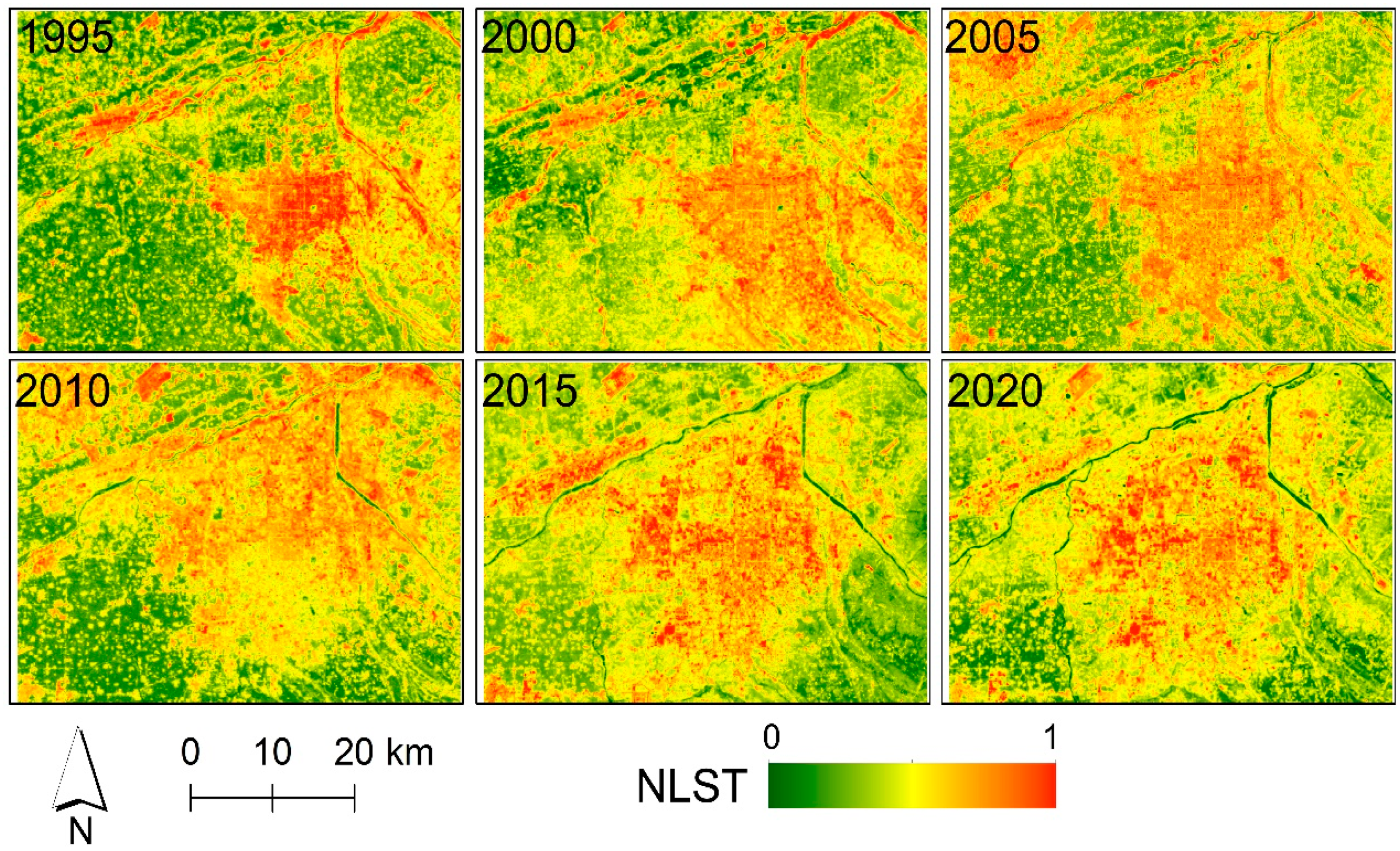
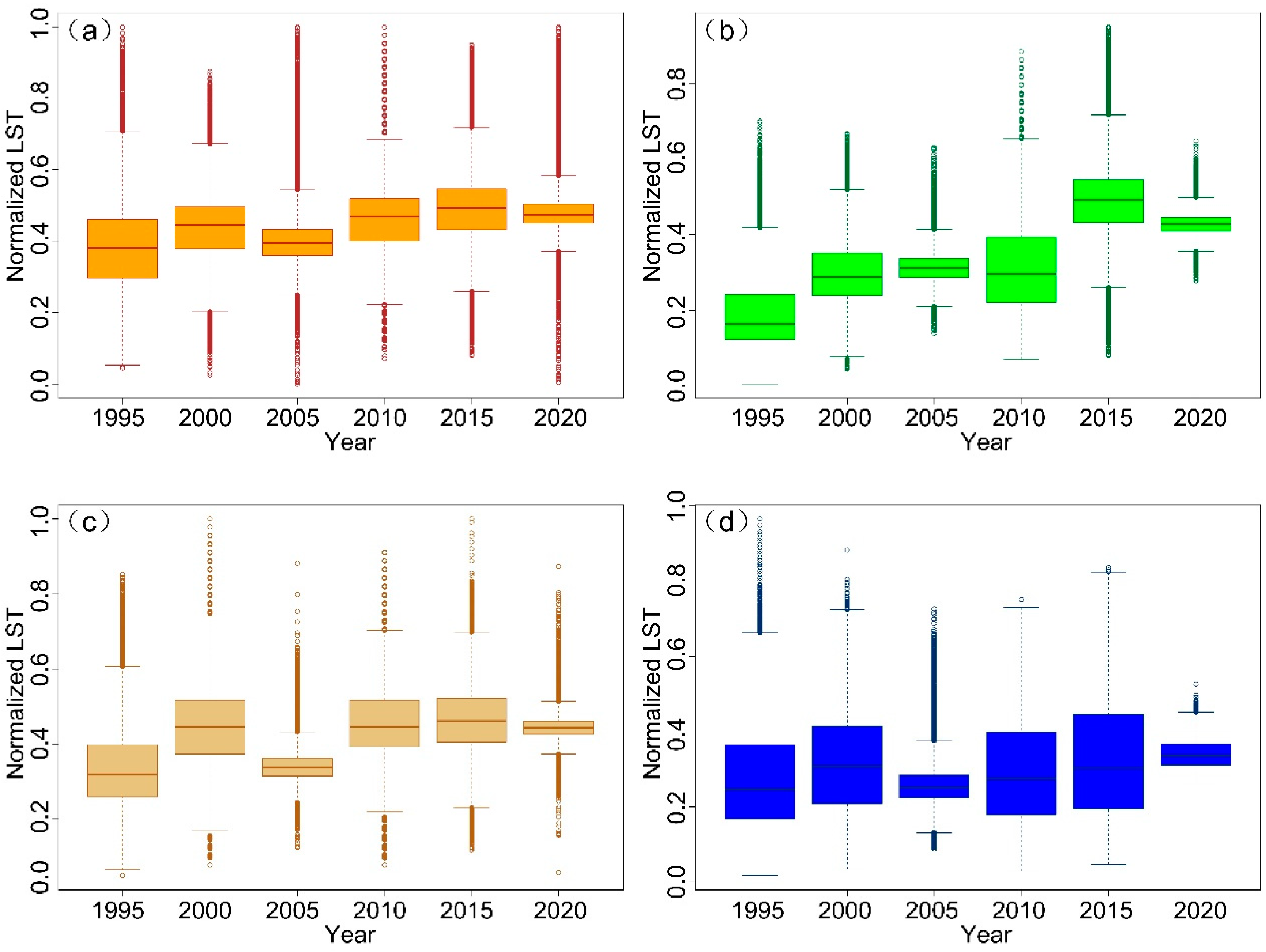
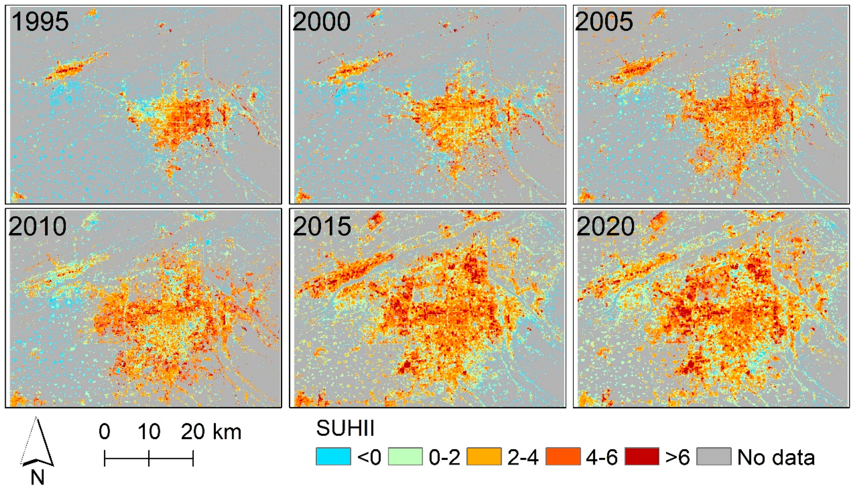
The average of NLST in built-up areas and bare land is consistently higher than vegetation and water bodies. Compared to impervious surfaces such as roads, pavements, buildings, and parking lots, vegetated areas can emit lower radiance, increase evapotranspiration, and provide shading from canopies, and thus, reduce their surrounding temperature [59,60,61]. The increasing trend of NLST across all land cover types indicates an overall trend of surface warming during the study period. The SUHII of the study area is 2.759 °C in 2020, which is comparable to other big cities in China. For example, the mean LST of impervious surface were 2.8 and 3.4 °C higher than the mean LST of green space in Guangzhou and Beijing, respectively [62,63]. Urbanization led to an expansion of built-up areas and increasing human activities in the study area. The increase in heat-absorbing manmade materials, reduction in natural vegetation, and increase in anthropogenic heat release during urbanization caused the increase in NLST across time [64].

The higher correlation between LST with NDISI than NDVI confirms earlier findings that built-up areas have a stronger impact on LST in comparison with green space [35,65]. The analysis results indicate that the correlation between NDISI and LST increases with an increase in window size, whereas the optimal grid cell size of the green space that influences LST effectively is from 210 to 240 m. The result agrees with findings of previous studies that used a comparable multi-scale grid analysis approach [66,67]. A previous study by Xiao et al. [66] reported that correlation between density of built-up areas and LST was enhanced as the size of analysis unit grew from 30 to 960 m in a UHI study in Beijing, China. The changing trend of the correlation between green space density and mean LST implies existence of a distance threshold for cooling effect of green space. Based on the analysis of air temperature recorded at weather stations, Myint et al. [67] also found that the correlation between impervious surfaces and maximum air temperatures decreased after reaching a window size of 210 m in Phoenix, Arizona, USA. The impacts of increasing urban green infrastructure on local meteorology have been simulated using statistical and numerical models in urban and green space planning for heat mitigation strategies [68]. The optimal cell grid size should be considered for the modeling of environmental parameters between LST and land cover. Grids with a coarse spatial resolution in numerical models may fail to capture the cooling effects of green areas [69].

The land cover configuration analysis reveals that large amounts of built-up area induced stronger heat island effects, while the shape of the built-up area had an insignificant effect on LST. Increasing the total area of green space significantly mitigated the negative impact of UHI in the study area. The influence of the shape and arrangement of green space on temperature reduction has been widely investigated and contrasting findings have been reported in case studies of different cities. Li found that LST increased significantly with higher patch density, given a fixed amount of greenspace in the Beijing metropolitan area [38]. In contrast, Peng et al. claimed a positive correlation between LST and the shape and fragmentation index of vegetated land in Beijing [70]. Asgarian found a complex patch shape with highly convoluted edges had stronger mitigating effects on land surface temperature in Isfahan, Iran [71]. Using analytical units with the largest size of 1080 × 1080 m, Zhou et al. reported that mean patch size and edge density of trees had negative and positive effects on LST in Sacramento, CA, USA with a Mediterranean climate with hot and dry summers, respectively [36]. With 240 × 240 m grids, Masoudi et al. [72] analyzed the complex relationship between green space pattern and LST in four major cities in Asia and found that configuration was not an influencing factor of LST in Kuala Lumpur and Hong Kong, while simply shaped, more aggregated, less fragmented patches of green space provided better cooling effects in Jakarta and Singapore. The analysis units varied from patches or census tracts to multi-scale grid cells in these studies. Since landscape metrics are sensitive to the size and shape of the calculation extent, the landscape metric values calculated using analysis units with different sizes or irregular shapes are incomparable [56,73,74]. The study by Estoque et al., which used the same analysis unit as the present study, revealed that aggregation had consistent and strong correlation with LST in the three Asian megacities, Bangkok, Jakarta, and Manila [34]. This agrees with our results that aggregated green space had better cooling effects than fragmented green space. However, Wesley and Brunsell claimed that the selection of window size in the above studies lacked biophysical justification and might fail to represent the characteristic scales of LST–green space interaction. They conducted a multi-resolution wavelet analysis to identify the dominant scales of LST variation for each image pixel and used them as the calculation extents of landscape metrics [74]. Despite the inconsistencies in the previous studies, the consensus is that the contribution of green space configuration to SUHI is weak, comparing with the percentage of vegetation [74].

In spite of these findings, several limitations of our study should be considered. The findings are limited to one inland city in northwestern China. The relationship between LST and spatial configurations of urban green space may vary in different cities. To fully understand the impacts of the spatial arrangement of urban land cover on LST, their relationship should be investigated by comparing multiples cities under different settings [75]. Moreover, only land cover characteristics were examined in this study; in addition to their spatial arrangements, the impact of other factors such as the functional types and heights of vegetation should also be investigated due to the cooling effects of green spaces in urban environments [76].

6. Conclusions

The spatiotemporal variations of the thermal environment and their relationships with land cover characteristics were investigated with remote sensing data in Xi’an, a fast-growing city in northwestern China. The land cover maps were classified and land surface temperature was estimated using Landsat imagery for six time periods with a five-year interval from 1995 to 2020. The built-up area increased from 413.74 to 1022.75 km², and the area of green space and water bodies significantly decreased from 1995 to 2020. An overall trend of surface warming was revealed during 1995–2020, with the increase in mean SUHII from 0.683 °C in 1995 to 2.759 °C in 2020. The effects of built-up areas and vegetated areas on LST were analyzed based on polygon grids at different spatial scales. The results indicated that the densities of built-up areas had a stronger impact on land surface temperature than green space. The correlation between NDISI and LST was enhanced with the enlargement of the grid cell size. The correlations between NDVI and LST reached their maxima at the grid cell sizes of 210 and 240 m. Increasing the total area and aggregation level of green space can mitigate the negative impact of urban heat islands. These results enhanced our understanding of spatiotemporal variations of thermal environment and their association with land cover features in an inland city with a temperate continental monsoon climate. The main findings can provide implications for urban planners on UHI mitigation and land resource utilization in the study area.

Our study confirmed that multi-scale analysis methods should be applied for the exploration of the impacts of land cover patterns on SUHI in future studies. Moreover, the impacts of the spatial arrangement and features of green space on urban thermal environment are complex and should be further investigated. The warming and cooling effects of land cover and their characteristics can be explored using climate and statistical model simulations for the building of sustainable and resilient urban landscapes [77,78,79].

References

1. DESA; UN. World Urbanization Prospects: The 2018 Revision; Department of Economic and Social Affairs: New York, NY, USA, 2019. [Google Scholar]
2. Foley, J.A.; DeFries, R.; Asner, G.P.; Barford, C.; Bonan, G.; Carpenter, S.R.; Chapin, F.S.; Coe, M.T.; Daily, G.C.; Gibbs, H.K.; et al. Global consequences of land use. Science 2005, 309, 570–574. [Google Scholar] [CrossRef] [PubMed] [Green Version]
3. Grimm, N.B.; Faeth, S.H.; Golubiewski, N.E.; Redman, C.L.; Wu, J.; Bai, X.; Briggs, J.M. Global change and the ecology of cities. Science 2008, 319, 756–760. [Google Scholar] [CrossRef] [PubMed] [Green Version]
4. Zhao, L.; Lee, X.; Smith, R.B.; Oleson, K. Strong contributions of local background climate to urban heat islands. Nature 2014, 511, 216–219. [Google Scholar] [CrossRef]
5. Voogt, J.A.; Oke, T.R. Thermal remote sensing of urban climates. Remote Sens. Environ. 2003, 86, 370–384. [Google Scholar] [CrossRef]
6. Weng, Q. Thermal infrared remote sensing for urban climate and environmental studies: Methods, applications, and trends. ISPRS J. Photogramm. Remote Sens. 2009, 64, 335–344. [Google Scholar] [CrossRef]
7. Fu, P.; Weng, Q. Consistent land surface temperature data generation from irregularly spaced Landsat imagery. Remote Sens. Environ. 2016, 184, 175–187. [Google Scholar] [CrossRef]
8. Zhou, D.; Xiao, J.; Bonafoni, S.; Berger, C.; Deilami, K.; Zhou, Y.; Frolking, S.; Yao, R.; Qiao, Z.; Sobrino, J.A. Satellite Remote Sensing of Surface Urban Heat Islands: Progress, Challenges, and Perspectives. Remote Sens. 2019, 11, 48. [Google Scholar] [CrossRef] [Green Version]
9. Deilami, K.; Kamruzzaman, M.; Liu, Y. Urban heat island effect: A systematic review of spatio-temporal factors, data, methods, and mitigation measures. Int. J. Appl. Earth Obs. Geoinf. 2018, 67, 30–42. [Google Scholar] [CrossRef]
10. Lu, L.; Weng, Q.; Guo, H.; Feng, S.; Li, Q. Assessment of urban environmental change using multi-source remote sensing time series (2000–2016): A comparative analysis in selected megacities in Eurasia. Sci. Total Environ. 2019, 684, 567–577. [Google Scholar] [CrossRef]
11. Firozjaei, M.K.; Kiavarz, M.; Alavipanah, S.K.; Lakes, T.; Qureshi, S. Monitoring and forecasting heat island intensity through multi-temporal image analysis and cellular automata-Markov chain modelling: A case of Babol city, Iran. Ecol. Indic. 2018, 91, 155–170. [Google Scholar] [CrossRef]
12. Simwanda, M.; Ranagalage, M.; Estoque, R.C.; Murayama, Y. Spatial analysis of surface urban heat islands in four rapidly growing African cities. Remote Sens. 2019, 11, 1645. [Google Scholar] [CrossRef] [Green Version]
13. Stewart, I.D. A systematic review and scientific critique of methodology in modern urban heat island literature. Int. J. Climatol. 2011, 31, 200–217. [Google Scholar] [CrossRef]
14. Sobrino, J.A.; Irakulis, I. A Methodology for Comparing the Surface Urban Heat Island in Selected Urban Agglomerations Around the World from Sentinel-3 SLSTR Data. Remote Sens. 2020, 12, 2052. [Google Scholar] [CrossRef]
15. Schwarz, N.; Lautenbach, S.; Seppelt, R. Exploring indicators for quantifying surface urban heat islands of European cities with MODIS land surface temperatures. Remote Sens. Environ. 2011, 115, 3175–3186. [Google Scholar] [CrossRef]
16. Stewart, I.D.; Oke, T.R. Local climate zones for urban temperature studies. Bull. Am. Meteorol. Soc. 2012, 93, 1879–1900. [Google Scholar] [CrossRef]
17. Rosentreter, J.; Hagensieker, R.; Waske, B. Towards large-scale mapping of local climate zones using multitemporal Sentinel 2 data and convolutional neural networks. Remote Sens. Environ 2020, 237, 12. [Google Scholar] [CrossRef]
18. Chen, X.; Zhang, Y. Impacts of urban surface characteristics on spatiotemporal pattern of land surface temperature in Kunming of China. Sustain. Cities Soc. 2017, 32, 87–99. [Google Scholar] [CrossRef] [Green Version]
19. Bechtel, B.; Demuzere, M.; Mills, G.; Zhan, W.; Sismanidis, P.; Small, C.; Voogt, J. SUHI analysis using Local Climate Zones—A comparison of 50 cities. Urban Clim. 2019, 28, 100451. [Google Scholar] [CrossRef]
20. Imhoff, M.L.; Zhang, P.; Wolfe, R.E.; Bounoua, L. Remote sensing of the urban heat island effect across biomes in the continental USA. Remote Sens. Environ 2010, 114, 504–513. [Google Scholar] [CrossRef] [Green Version]
21. Peng, S.; Piao, S.; Ciais, P.; Friedlingstein, P.; Ottle, C.; Bréon, F.-M.; Nan, H.; Zhou, L.; Myneni, R.B. Surface urban heat island across 419 global big cities. Environ. Sci. Technol. 2012, 46, 696–703. [Google Scholar] [CrossRef]
22. Zhou, D.; Zhao, S.; Liu, S.; Zhang, L.; Zhu, C. Surface urban heat island in China’s 32 major cities: Spatial patterns and drivers. Remote Sens. Environ 2014, 152, 51–61. [Google Scholar] [CrossRef]
23. Firozjaei, M.K.; Weng, Q.; Zhao, C.; Kiavarz, M.; Lu, L.; Alavipanah, S.K. Surface anthropogenic heat islands in six megacities: An assessment based on a triple-source surface energy balance model. Remote Sens. Environ 2020, 242, 111751. [Google Scholar] [CrossRef]
24. Weng, Q.H.; Lu, D.S.; Schubring, J. Estimation of land surface temperature-vegetation abundance relationship for urban heat island studies. Remote Sens. Environ. 2004, 89, 467–483. [Google Scholar] [CrossRef]
25. Li, J.; Song, C.; Cao, L.; Zhu, F.; Meng, X.; Wu, J. Impacts of landscape structure on surface urban heat islands: A case study of Shanghai, China. Remote Sens. Environ. 2011, 115, 3249–3263. [Google Scholar] [CrossRef]
26. Gogoi, P.P.; Vinoj, V.; Swain, D.; Roberts, G.; Dash, J.; Tripathy, S. Land use and land cover change effect on surface temperature over Eastern India. Sci. Rep. 2019, 9, 10. [Google Scholar] [CrossRef] [Green Version]
27. Guha, S.; Govil, H.; Diwan, P. Analytical study of seasonal variability in land surface temperature with normalized difference vegetation index, normalized difference water index, normalized difference built-up index, and normalized multiband drought index. J. Appl. Remote Sens. 2019, 13, 16. [Google Scholar] [CrossRef] [Green Version]
28. Logan, T.M.; Zaitchik, B.; Guikema, S.; Nisbet, A. Night and day: The influence and relative importance of urban characteristics on remotely sensed land surface temperature. Remote Sens. Environ. 2020, 247, 25. [Google Scholar] [CrossRef]
29. Song, J.C.; Chen, W.; Zhang, J.J.; Huang, K.; Hou, B.Y.; Prishchepov, A.V. Effects of building density on land surface temperature in China: Spatial patterns and determinants. Landsc. Urban Plan. 2020, 198, 13. [Google Scholar] [CrossRef]
30. Weng, Q.; Liu, H.; Lu, D. Assessing the effects of land use and land cover patterns on thermal conditions using landscape metrics in city of Indianapolis, United States. Urban Ecosyst. 2007, 10, 203–219. [Google Scholar] [CrossRef]
31. Liu, H.; Weng, Q. Scaling effect on the relationship between landscape pattern and land surface temperature: A case study of Indianapolis, United States. Photogramm. Eng. Remote Sens. 2009, 75, 291–304. [Google Scholar] [CrossRef] [Green Version]
32. Xie, M.M.; Chen, J.; Zhang, Q.Y.; Li, H.T.; Fu, M.C.; Breuste, J. Dominant landscape indicators and their dominant areas influencing urban thermal environment based on structural equation model. Ecol. Indic. 2020, 111, 12. [Google Scholar] [CrossRef]
33. Connors, J.P.; Galletti, C.S.; Chow, W.T.L. Landscape configuration and urban heat island effects: Assessing the relationship between landscape characteristics and land surface temperature in Phoenix, Arizona. Landsc. Ecol. 2013, 28, 271–283. [Google Scholar] [CrossRef]
34. Estoque, R.C.; Murayama, Y.; Myint, S.W. Effects of landscape composition and pattern on land surface temperature: An urban heat island study in the megacities of Southeast Asia. Sci. Total Environ. 2017, 577, 349–359. [Google Scholar] [CrossRef] [PubMed]
35. Zhou, W.; Wang, J.; Cadenasso, M.L. Effects of the spatial configuration of trees on urban heat mitigation: A comparative study. Remote Sens. Environ. 2017, 195, 1–12. [Google Scholar] [CrossRef]
36. Ma, Q.; Wu, J.; He, C. A hierarchical analysis of the relationship between urban impervious surfaces and land surface temperatures: Spatial scale dependence, temporal variations, and bioclimatic modulation. Landsc. Ecol. 2016, 31, 1139–1153. [Google Scholar] [CrossRef]
37. Luan, X.; Yu, Z.; Zhang, Y.; Wei, S.; Miao, X.; Huang, Z.Y.X.; Teng, S.N.; Xu, C. Remote sensing and social sensing data reveal scale-dependent and system-specific strengths of urban heat island determinants. Remote Sens. 2020, 12, 391. [Google Scholar] [CrossRef] [Green Version]
38. Li, X.M.; Zhou, W.Q.; Ouyang, Z.Y.; Xu, W.H.; Zheng, H. Spatial pattern of greenspace affects land surface temperature: Evidence from the heavily urbanized Beijing metropolitan area, China. Landsc. Ecol. 2012, 27, 887–898. [Google Scholar] [CrossRef]
39. Guo, L.J.; Liu, R.M.; Men, C.; Wang, Q.R.; Miao, Y.X.; Zhang, Y. Quantifying and simulating landscape composition and pattern impacts on land surface temperature: A decadal study of the rapidly urbanizing city of Beijing, China. Sci. Total Environ. 2019, 654, 430–440. [Google Scholar] [CrossRef]
40. Xu, M.; Hong, B.; Jiang, R.; An, L.; Zhang, T. Outdoor thermal comfort of shaded spaces in an urban park in the cold region of China. Build. Environ. 2019, 155, 408–420. [Google Scholar] [CrossRef]
41. Yang, Y.; Li, W. The evolution of the ecological footprint and its relationship with the urban development of megacities in Western China: The case of Xi’an. J. Environ. Manag. 2019, 243, 463–471. [Google Scholar] [CrossRef]
42. Weng, Q.H.; Firozjaei, M.K.; Sedighi, A.; Kiavarz, M.; Alavipanah, S.K. Statistical analysis of surface urban heat island intensity variations: A case study of Babol city, Iran. Giscience Remote Sens. 2019, 56, 576–604. [Google Scholar] [CrossRef]
43. Xu, H. Analysis of impervious surface and its impact on urban heat environment using the normalized difference impervious surface index (NDISI). Photogramm. Eng. Remote Sens. 2010, 76, 557–565. [Google Scholar] [CrossRef]
44. Lu, L.; Kuenzer, C.; Wang, C.; Guo, H.; Li, Q. Evaluation of Three MODIS-Derived Vegetation Index Time Series for Dryland Vegetation Dynamics Monitoring. Remote Sens. 2015, 7, 7597–7614. [Google Scholar] [CrossRef] [Green Version]
45. Li, Q.; Lu, L.; Wang, C.; Li, Y.; Sui, Y.; Guo, H. MODIS-derived spatiotemporal changes of major lake surface areas in arid Xinjiang, China, 2000–2014. Water 2015, 7, 5731–5751. [Google Scholar] [CrossRef]
46. Olofsson, P.; Foody, G.M.; Herold, M.; Stehman, S.V.; Woodcock, C.E.; Wulder, M.A. Good practices for estimating area and assessing accuracy of land change. Remote Sens. Environ. 2014, 148, 42–57. [Google Scholar] [CrossRef]
47. Wickham, J.D.; Stehman, S.V.; Gass, L.; Dewitz, J.; Fry, J.A.; Wade, T.G. Accuracy assessment of NLCD 2006 land cover and impervious surface. Remote Sens. Environ. 2013, 130, 294–304. [Google Scholar] [CrossRef]
48. Finegold, Y.; Ortmann, A.; Lindquist, E.; d’Annunzio, R.; Sandker, M. Map Accuracy Assessment and Area Estimation: A Practical Guide; Food and Agriculture Organization of the United Nations: Rome, Italy, 2016. [Google Scholar]
49. Shih, H.-C.; Stow, D.A.; Tsai, Y.H. Guidance on and comparison of machine learning classifiers for Landsat-based land cover and land use mapping. Int. J. Remote Sens. 2019, 40, 1248–1274. [Google Scholar] [CrossRef]
50. Sobrino, J.A.; Raissouni, N.; Li, Z.-L. A Comparative Study of Land Surface Emissivity Retrieval from NOAA Data. Remote Sens. Environ. 2001, 75, 256–266. [Google Scholar] [CrossRef]
51. Sobrino, J.A.; Jiménez-Muñoz, J.C.; Paolini, L. Land surface temperature retrieval from LANDSAT TM 5. Remote Sens. Environ. 2004, 90, 434–440. [Google Scholar] [CrossRef]
52. Sobrino, J.A.; Jimenez-Munoz, J.C.; Soria, G.; Romaguera, M.; Guanter, L.; Moreno, J.; Plaza, A.; Martinez, P. Land surface emissivity retrieval from different VNIR and TIR sensors. IEEE Trans. Geosci. Remote Sens. 2008, 46, 316–327. [Google Scholar] [CrossRef]
53. Weng, Q.; Rajasekar, U.; Hu, X. Modeling urban heat islands and their relationship with impervious surface and vegetation abundance by using ASTER images. IEEE Trans. Geosci. Remote Sens. 2011, 49, 4080–4089. [Google Scholar] [CrossRef]
54. Estoque, R.C.; Murayama, Y. Monitoring surface urban heat island formation in a tropical mountain city using Landsat data (1987–2015). Isprs J. Photogramm. Remote Sens. 2017, 133, 18–29. [Google Scholar] [CrossRef]
55. McGarigal, K.; Cushman, S.A.; Ene, E. FRAGSTATS v4:Spatial Pattern Analysis Program for Categorical and Continuous Maps. Available online: http://www.umass.edu/landeco/research/fragstats/fragstats.html (accessed on 15 December 2019).
56. Amiri, R.; Weng, Q.; Alimohammadi, A.; Alavipanah, S.K. Spatial–temporal dynamics of land surface temperature in relation to fractional vegetation cover and land use/cover in the Tabriz urban area, Iran. Remote Sens. Environ. 2009, 113, 2606–2617. [Google Scholar] [CrossRef]
57. Guo, G.; Wu, Z.; Xiao, R.; Chen, Y.; Liu, X.; Zhang, X. Impacts of urban biophysical composition on land surface temperature in urban heat island clusters. Landsc. Urban Plan. 2015, 135, 1–10. [Google Scholar] [CrossRef]
58. Jones, H.G.; Sirault, X.R.R. Scaling of thermal images at different spatial resolution: The mixed pixel problem. Agronomy 2014, 4, 380–396. [Google Scholar] [CrossRef] [Green Version]
59. Bowler, D.E.; Buyung-Ali, L.; Knight, T.M.; Pullin, A.S. Urban greening to cool towns and cities: A systematic review of the empirical evidence. Landsc. Urban Plan. 2010, 97, 147–155. [Google Scholar] [CrossRef]
60. Schwarz, N.; Schlink, U.; Franck, U.; Grossmann, K. Relationship of land surface and air temperatures and its implications for quantifying urban heat island indicators-An application for the city of Leipzig (Germany). Ecol. Indic. 2012, 18, 693–704. [Google Scholar] [CrossRef]
61. Peres, L.D.; de Lucena, A.J.; Rotunno, O.C.; Franca, J.R.D. The urban heat island in Rio de Janeiro, Brazil, in the last 30 years using remote sensing data. Int. J. Appl. Earth Obs. Geoinf. 2018, 64, 104–116. [Google Scholar] [CrossRef]
62. Song, J.; Du, S.; Feng, X.; Guo, L. The relationships between landscape compositions and land surface temperature: Quantifying their resolution sensitivity with spatial regression models. Landsc. Urban Plan. 2014, 123, 145–157. [Google Scholar] [CrossRef]
63. Sun, Q.; Wu, Z.; Tan, J. The relationship between land surface temperature and land use/land cover in Guangzhou, China. Environ. Earth Sci. 2012, 65, 1687–1694. [Google Scholar] [CrossRef]
64. Mohajerani, A.; Bakaric, J.; Jeffrey-Bailey, T. The urban heat island effect, its causes, and mitigation, with reference to the thermal properties of asphalt concrete. J. Environ. Manag. 2017, 197, 522–538. [Google Scholar] [CrossRef] [PubMed]
65. Yuan, F.; Bauer, M.E. Comparison of impervious surface area and normalized difference vegetation index as indicators of surface urban heat island effects in Landsat imagery. Remote Sens. Environ. 2007, 106, 375–386. [Google Scholar] [CrossRef]
66. Xiao, R.-b.; Ouyang, Z.-y.; Zheng, H.; Li, W.-f.; Schienke, E.W.; Wang, X.-k. Spatial pattern of impervious surfaces and their impacts on land surface temperature in Beijing, China. J. Environ. Sci. 2007, 19, 250–256. [Google Scholar] [CrossRef]
67. Myint, S.W.; Brazel, A.; Okin, G.; Buyantuyev, A. Combined effects of impervious surface and vegetation cover on air temperature variations in a rapidly expanding desert city. GIScience Remote Sens. 2010, 47, 301–320. [Google Scholar] [CrossRef]
68. Sharma, A.; Conry, P.; Fernando, H.J.S.; Hamlet, A.F.; Hellmann, J.J.; Chen, F. Green and cool roofs to mitigate urban heat island effects in the Chicago metropolitan area: Evaluation with a regional climate model. Environ. Res. Lett. 2016, 11, 064004. [Google Scholar] [CrossRef]
69. Arghavani, S.; Malakooti, H.; Ali Akbari Bidokhti, A.-A. Numerical assessment of the urban green space scenarios on urban heat island and thermal comfort level in Tehran Metropolis. J. Clean. Prod. 2020, 261, 121183. [Google Scholar] [CrossRef]
70. Peng, J.; Xie, P.; Liu, Y.; Ma, J. Urban thermal environment dynamics and associated landscape pattern factors: A case study in the Beijing metropolitan region. Remote Sens. Environ. 2016, 173, 145–155. [Google Scholar] [CrossRef]
71. Asgarian, A.; Amiri, B.J.; Sakieh, Y. Assessing the effect of green cover spatial patterns on urban land surface temperature using landscape metrics approach. Urban Ecosyst. 2015, 18, 209–222. [Google Scholar] [CrossRef]
72. Masoudi, M.; Tan, P.Y.; Liew, S.C. Multi-city comparison of the relationships between spatial pattern and cooling effect of urban green spaces in four major Asian cities. Ecol. Indic. 2019, 98, 200–213. [Google Scholar] [CrossRef]
73. Wu, J. Effects of changing scale on landscape pattern analysis: Scaling relations. Landsc. Ecol. 2004, 19, 125–138. [Google Scholar] [CrossRef]
74. Wesley, E.J.; Brunsell, N.A. Greenspace Pattern and the Surface Urban Heat Island: A Biophysically-Based Approach to Investigating the Effects of Urban Landscape Configuration. Remote Sens. 2019, 11, 2322. [Google Scholar] [CrossRef] [Green Version]
75. Kabisch, N.; Qureshi, S.; Haase, D. Human–environment interactions in urban green spaces—A systematic review of contemporary issues and prospects for future research. Environ. Impact Assess. Rev. 2015, 50, 25–34. [Google Scholar] [CrossRef]
76. Yu, Q.Y.; Acheampong, M.; Pu, R.L.; Landry, S.M.; Ji, W.J.; Dahigamuwa, T. Assessing effects of urban vegetation height on land surface temperature in the City of Tampa, Florida, USA. Int. J. Appl. Earth Obs. Geoinf. 2018, 73, 712–720. [Google Scholar] [CrossRef]
77. Mijani, N.; Alavipanah, S.K.; Firozjaei, M.K.; Arsanjani, J.J.; Hamzeh, S.; Weng, Q. Modeling outdoor thermal comfort using satellite imagery: A principle component analysis-based approach. Ecol. Indic. 2020, 117, 106555. [Google Scholar] [CrossRef]
78. Sodoudi, S.; Zhang, H.; Chi, X.; Müller, F.; Li, H. The influence of spatial configuration of green areas on microclimate and thermal comfort. Urban For. Urban Green. 2018, 34, 85–96. [Google Scholar] [CrossRef]
79. Osborne, P.E.; Alvares-Sanches, T. Quantifying how landscape composition and configuration affect urban land surface temperatures using machine learning and neutral landscapes. Comput. Environ. Urban Syst. 2019, 76, 80–90. [Google Scholar] [CrossRef]
Figure 1. Geographic location of the study area. The satellite image is false color composite of Landsat 8 acquired on 9 April 2020.
Remotesensing 12 02713 g001
Figure 2. Land cover classification map in the study area for six time periods from 1995 to 2020.
Remotesensing 12 02713 g002
Figure 3. Normalized land surface temperature in the study area for six time periods from 1995 to 2020.
Remotesensing 12 02713 g003
Figure 4. Box plots of normalized land surface temperature for different land cover types. (a) Built-up area, (b) green space, (c) bare land, and (d) water.
Remotesensing 12 02713 g004
Figure 5. Spatial pattern of SUHII (°C) in the study area for six time periods from 1995 to 2020.
Remotesensing 12 02713 g005
Figure 6. Correlation between NDISI and NDVI and mean LST across grid cell sizes. All correlations were significant at the 0.01 level (2-tailed). The orange and green lines represent NDISI and NDVI, respectively.
Remotesensing 12 02713 g006