The Determination of Effective Beamwidth of Ku Band Profiling Radar Based on Waveform Matching Method in the Boreal Forest of Finland

Abstract

Radar scientists typically define the radar beamwidth as a half-power beamwidth (HPBW) in the main lobe of the antenna pattern. However, the microwave radiations outside radar HPBW might also backscatter into the radar receiver and change the distribution of the received signal. To determine an actual and effective beamwidth illuminated on the measured targets, we first generate the simulated-waveforms derived from coincident lidar points and radar equation and then develop a waveform matching method to seek out an optimal beamwidth based on the 95% threshold of correlation coefficients between radar waveforms and the simulated-waveforms. The 8565 measurements of a Ku-band profiling radar named Tomoradar and coincident lidar data in a widespread heterogeneous forest area of southern Finland are employed for resolving the effective beamwidth. The results reveal that about 97% of the effective beamwidth are larger than Tomoradar HPBW, but the effective beamwidth could be changeable for each measurement due to variations in the scattering properties of vegetation. Thus, a fixed average effective beamwidth (AEBW) with 0.1-degree resolution is introduced to determine Tomoradar cone according to the effective beamwidth and corresponding proportions. We discover that Tomoradar AEBW is approximately approaching to 8°, which is larger than Tomoradar HPBW of 6°. If we regard AEBW as the actual Tomoradar beamwidth rather than HPBW, the simulated-waveforms have substantially stronger correlation strength with Tomoradar waveforms, and canopy tops derived from lidar data within Tomoradar AEBW are much closer to those extracted from Tomoradar waveforms. The results demonstrate that radar AEBW is a more appropriate reference for designing radar antenna and selecting the region size of validation data such as lidar points or the ground truth. However, considering that radar AEBW is variable for different radar antenna pattern, we suggest that actual radar beamwidth should be defined with a fraction of total radiation energy within radar AEBW, just like the definition of laser divergence of lidar based on the percentage of transmitted laser energy. In this paper, for a forest inventory research case, the fraction of total radiation energy within the AEBW for radar system is supposed to be 91%.

1. Introduction

Forest covers approximately 30 percent of the global land area and plays an essential role in the natural circulation of carbon and mitigation of climate change. Many remote sensing instruments, including active and passive sensors, such as optical sensors, synthetic aperture radar (SAR), lidar, and microwave radar, are capable of exploring spatially continuous properties of forest structure over large areas in a rapid manner [1,2,3,4]. Due to its all-weather imaging capability, satellite SAR is more feasible for wide-area mapping in a much efficient manner. It provides continuous forest mapping and updating on a global scale, in addition, SAR can provide significantly higher sensitivity to the vertical forest elements due to the ability to penetrate through the vegetation layer and interact with forest vertical structure components comparing with other optical passive/active remote sensing techniques. SAR tomography has emerged in the last years as a vital tool for the investigation of forested areas by its capability to resolve the vertical structure of the target [5,6,7]. They have become significant instruments in the investigation of the vertical canopy structure.

Stand profiles that present tree height and density in the forest using helicopter-borne frequency-modulated continuous waveform (FMCW) microwave radar were also reported by [4,8,9]. A light-weighted Ku-band (FM-CW) profiling radar, named Tomoradar, was developed by the Finnish Geospatial Research Institute (FGI) to collect full polarization backscattered signal from the boreal forest and investigate the vertical canopy structure information. Tomoradar can provide four linear polarization measuring capabilities in Ku band based bistatic configuration with 15 cm range solution, to improve the understanding of the radar backscatter response for forestry mapping and inventories. Subsequent studies on forest inventory, especially for vertical forest structure using FMCW radar data have been conducted in the past few years [10,11,12,13,14].

The principle of FMCW radar is straightforward: an FMCW radar transmits a frequency-modulated (FM) signal (normally linear FM) with a given bandwidth (BW). It receives an attenuated copy of the transmitted signal representing the backscatters from a target. By multiplying the transmitted signal with the received signal, an intermediate frequency (IF) difference signal containing a beat frequency is generated, and the beat frequency is proportional to the range. The IF signal is then amplified and digitalized by an oscilloscope device [9]. Due to the linear modulation mode, the beat frequency is directly proportional to the two-way range. The BW (a few gigahertzes) of an FMCW system results in a theoretical range resolution even close to pulsed lidar [9,15]. FMCW radar offers another advantage by providing accurate high range resolution measurements without requiring a high sample rate analogue-to-digital converter since the range measurement is achieved from frequency domain by fast Fourier transform (FFT) process but not in the time domain. Due to the combination of excellent range resolution and good penetration in the operating radio frequency, the FMCW radar technique is extensively utilized by various research areas ranging from forest [16,17], snow, and ice [18], to human–computer interactions [19,20].

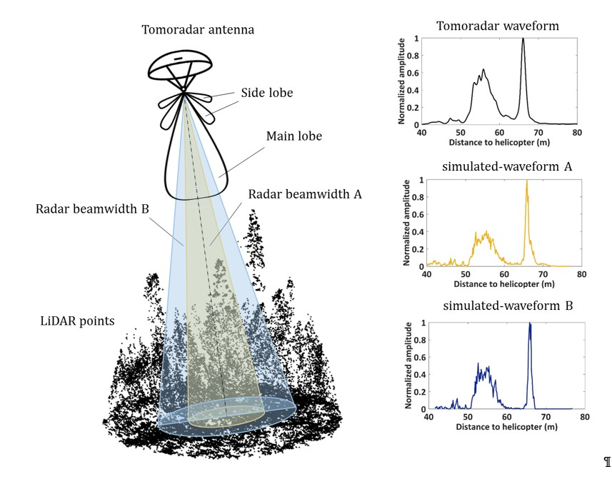
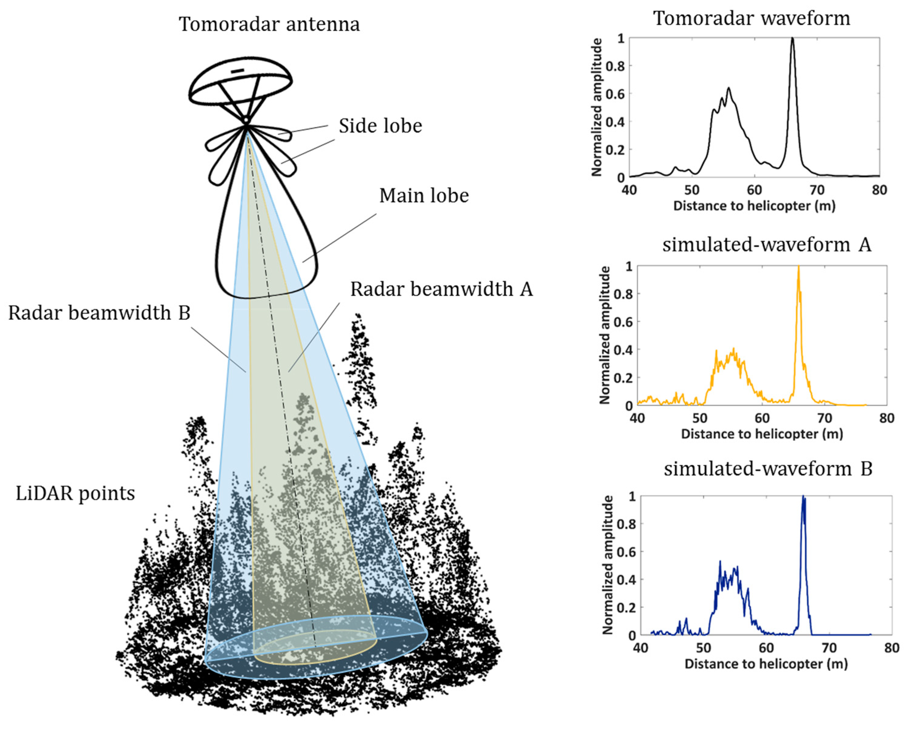
The FMCW radars transmit microwave radiations within a cone into the vegetation and receive backscattered energy from the surface of the plant. The cone is usually defined with a typical antenna beamwidth represented by the angular separation between two half-power (−3 dB) points of the main lobe [21]. Such half-power beamwidth (HPBW) is usually treated as the beamwidth during the design of a radar antenna for remote sensing. Meanwhile, the footprint size is also traditionally described to be the illuminated area on the ground within the field of view subtended by the HPBW, which is an essential conception to better understanding what the radar can observe and measure [22].

However, it is probably incorrect to choose HPBW as the beamwidth. The microwave energies outside the HPBW might also backscatter off the targets nearby and be collected by the radar receiver, causing the undesired signals that may conceal weaker returns from the more distant targets in the radar HPBW. The potential impact of backscattered energy outside radar HPBW is dependent on the relative strength of an antenna pattern and the scattering property of the measured targets beyond HPBW. These unwanted radiations in unexpected directions could originate from outside HPBW in the main lobe, even in the side lobe, which would change the distributions of backscattered signal and produce some unpredictable errors for the retrieval results. For example, Li found the antenna side lobe effect on the atmospheric temperature and water vapor density in ground-based microwave remote sensing of the atmosphere [23]. Kwok analyzed the effects of radar side lobes on snow depth retrievals from operation IceBridge [18] thoroughly. Feng and Chen found that the microwave radiations outside HPBW created an indecipherable impact on the accuracy of the canopy top [12]. These investigations demonstrate that it is unsuitable to only depend on HBPW when we design the beamwidth of the radar antenna and determine the footprint size or the region scope of validation data such as lidar data and the ground truth.

Therefore, it is necessary to resolve such actual radar beamwidth, defined as an effective beamwidth in this paper, to provide a piece of evidence in the design of radar antenna and the determination of footprint size. Nevertheless, there is no deterministic answer for ascertaining the effective beamwidth due to the missing of synergistic data and sensors. Until recently, the availability of the data of both radar and lidar on the same forest targets as close as possible on a single airborne platform under identical conditions (for example, observation angle, operation height, and aircraft vibration) offers an excellent opportunity to scientists to try to tackle this problem.

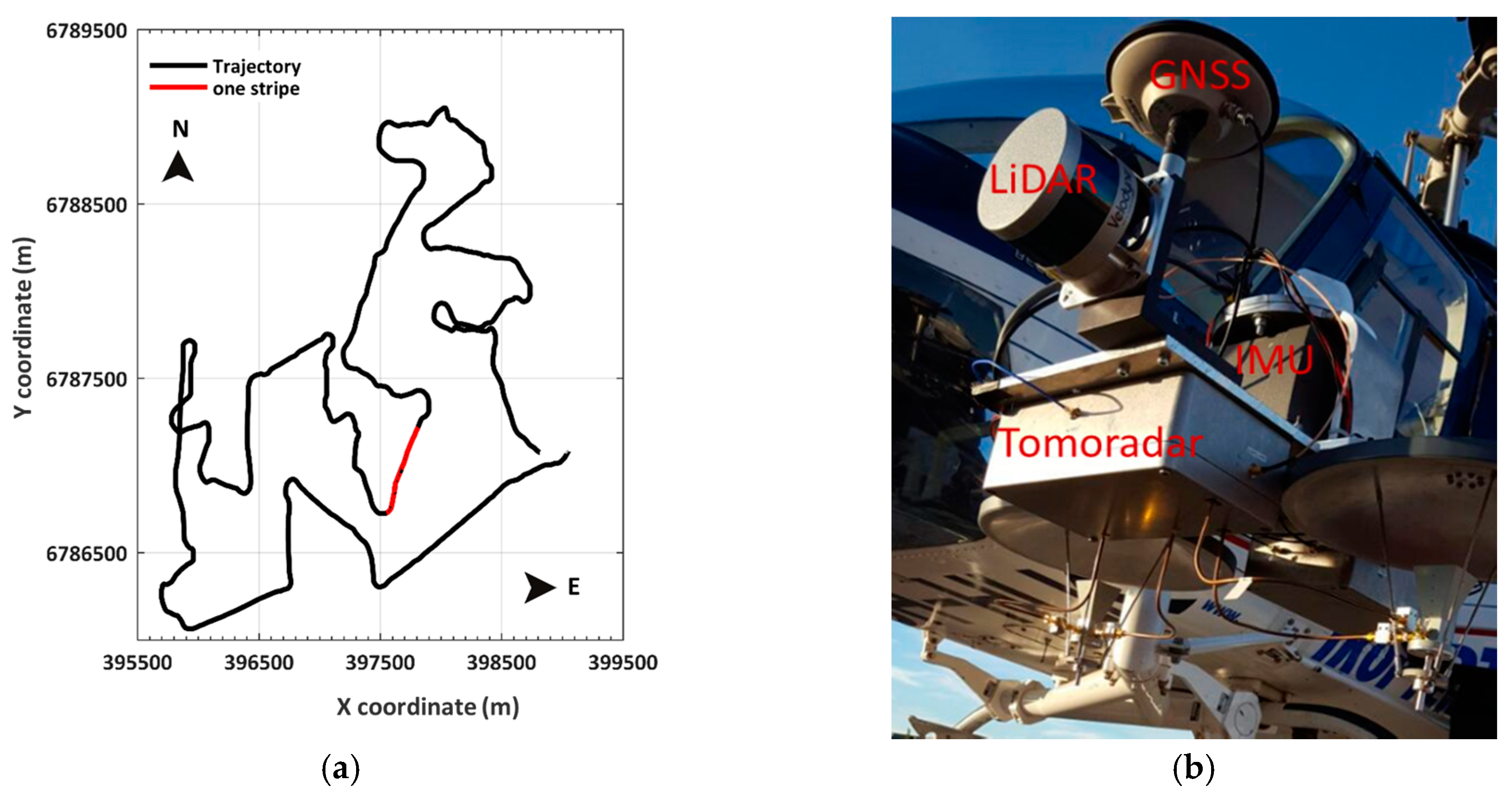
The coincident lidar data are simultaneously collected by a Velodyne VLP-16 lidar on the identical platform with Tomoradar. The major difference between Tomoradar and other FMCW radars, for example, radar systems for ice and snow application, is that the HPBW is very narrow, more specific, 6 degrees. The half-power beamwidth for snow investigation FMCM radar was tens of degrees, for example, 45° in [15]. It is well known that significant leakage will scatter from nearby environmental reflections even if antenna components are perfect for FMCW radar. Normally, higher than 100 dB leakage rejection is anticipated to achieve satisfactory performance. However, in Tomoradar, the vertical forest structure is more complex relative to the topography of snow coverage or ice sheet. However, the HPBW is considerably narrower, and the employed antenna is still a trade-off between theoretical investigation and practical product. Thus, in this research, we utilize the unique opportunity to investigate the synergic data both from radar and lidar for the following specific technical issues: How to determine the effective beamwidth of the profile radar for forestry inventory research rather than directly use HPBW noted by the datasheet, and to understand the microwave propagation within forest better. In other words, this research tries to tackle how the significant leakage scattered from the nearby forest environment outside of the cone defined by the HPBW will affect the final measurement.

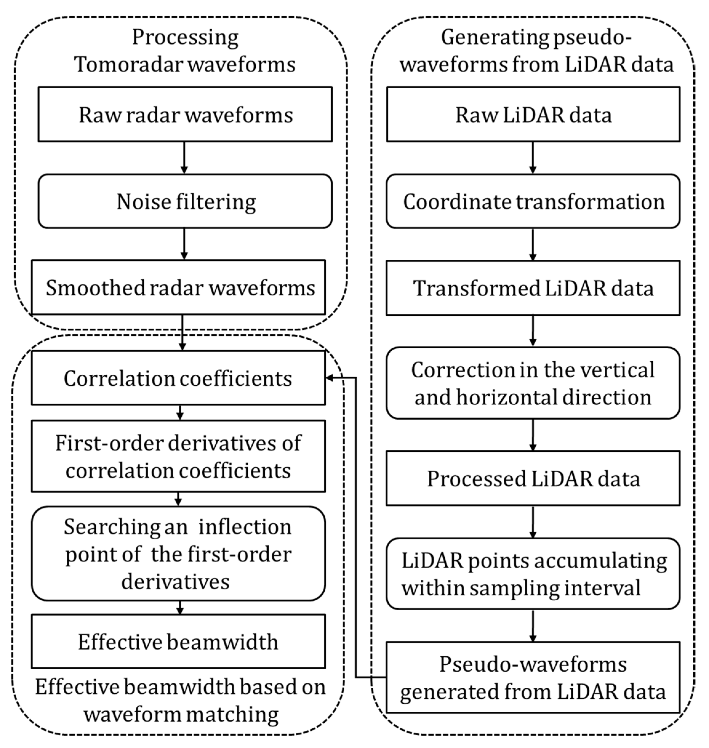
The subject of this paper is to determine the effective beamwidth based on the waveform matching technique analogously used in the large-footprint waveform lidar [16,24]. We utilized 8565 Tomoradar waveforms from one stripe collected in a test field in southern Finland and corresponding simulated-waveforms generated from coincident lidar data within various radar beamwidth settings to compute their correlation coefficients. By searching the best matching point with the distinctly slow growth of correlation coefficients, the effective beamwidth is resolved for each Tomoradar measurement. Meanwhile, an average effective beamwidth for all Tomoradar measurements is estimated as the actual Tomoradar beamwidth, and a visual comparison of canopy tops extracted from Tomoradar waveforms, lidar data within the average effective beamwidth, and HPBW is presented.

The rest of this paper is organized as the following: Section 2 describes the study area, Tomoradar waveforms, and lidar data, and illustrates the methods on the derivation of the effective beamwidth; Section 3 expounds the results and discussions about the effective beamwidth; finally, the conclusions are drawn in Section 4.

2. Materials and Methods

2.1. Study Area

The study area is located at Evo in southern Finland (61°19′N, 25°11′E). The test site comprises three sections: east section, west section and south section, and investigational data in this paper are selected from one stripe in the west section (Figure 1a). It is a straight line trajectory when the helicopter can fly as horizontal as possible with minor turbulence to keep observing the boreal forest in the nadir direction steadily. Different from an entirely homogenous managed forest, this site is a popular recreation area and includes Scots pine, Norway spruce, and birch. Both Tomoradar and Velodyne VLP-16 lidar were mounted on an extended arm of a Bell 206 helicopter with a zero degree incidence angle (i.e., with the antenna pointing down as Figure 1b presents) at a flight height of 60–100 m. In addition, a Global Navigation Satellite System and an Inertial Measurement Unit (GNSS-IMU) were attached on the frame to supply the positions and attitude angles during flight campaigns of the helicopter. The Tomoradar and lidar measurements were time-tagged with GPS time and coincided in a centimeter-level manner. The suites of all instruments on the helicopter are presented in Figure 1b [10]. The field test was carried in the autumn of 2016 under partly cloudy conditions.

Figure 1. (a) Trajectory diagram in the West section of the study area (black line), and a route of investigated data in one stripe (red line). The locations of trajectory are depicted in the local east, north, and up (ENU) coordinates; (b) the suites of all instruments on the Bell 206 helicopter: Tomoradar, lidar, and GNSS-IMU.

2.2. Tomoradar Waveforms

The Tomoradar transmitting antenna emits Ku-band microwave radiation with a central frequency of 14 GHz and a half-beamwidth of 3° (−3 dB). The receiving antenna captures the backscattered signals from measured targets in nadir direction four polarization modes (VV, VH, HV, and HH), and converts them into waveforms with a range resolution of 15 centimeters. The Radar return depending on (a) target orientation (aspect angle) and distance (range), (b) target environment (other objects nearby; location relative to the earth’s surface), (c) propagation characteristics of the path (rain, snow, or foliage attenuation), (d) antenna characteristics (polarization, beam width, and sidelobe level), and (e) transmitter (Tx) and receiver (Rx) characteristics. Raw Tomoradar waveforms are expressed as a distance-resolved amplitude of backscattered microwave radiation reflected from the canopy surface, inner layers, and the underlying ground [13,17]. The 8565 Tomoradar measurements with an along-track distance of approximately 600 m, then a spatial interval of 7 centimeters on the ground level were investigated to estimate the effective beamwidth of Tomoradar.

2.3. Lidar Data

The Velodyne VLP-16 lidar instantaneously generates 16 parallel scan lines with a 30° along-track field of view (FOV) of ±15° forward and backward on the ground and footprint size of 12.7 mm × 9.5 mm on the exit and enables measurements of about 300,000 data points per second and 360° across-track FOV. For our selected stripe, the average lidar point density was approximately 36 points per square meter, which corresponds to an average separation between lidar points of about 20 centimeters. The high-density lidar data preferably represent a three-dimensional distribution that illustrates the spatial heights of canopy and ground. All lidar points are converted in WGS-84 georeferenced system.

2.4. Methods

The Tomoradar waveforms represent the vertical distribution of Ku-band microwave radiation backscattered from targets across and along the beam path. Their shapes primarily rely on Radar cross section (RCS) of the targets from canopy to ground within the Tomoradar cone. A simulated-waveform generated from lidar points (mentioned in Section 2.4.2) is a demonstration of the vertical distribution of backscattering surface from the canopy to the ground, and it is anticipated to be likely similar to the captured Tomoradar waveform. As for each Tomoradar measurement, the resemblance extent between Tomoradar waveform and simulated-waveform is strongly dependent on the magnitude of the Tomoradar antenna pattern. Therefore, we provide various simulated-waveforms from lidar points within various Tomoradar beamwidth and determine an effective beamwidth by comparing the resemblance extent between the simulated-waveforms and the Tomoradar waveforms based on waveform matching method (mentioned in Section 2.4.3).

According to descriptions of raw Tomoradar waveforms and lidar data, the detailed schematic diagram of deriving the effective beamwidth of Ku-band profiling radar is presented in Figure 2. The methodology is employed by implementing three processing steps: (a) processing Tomoradar waveforms; (b) generating simulated-waveforms from lidar data; and (c) determining the effective beamwidth based on waveform matching method.

Figure 2. The flowchart of determining the effective beamwidth of Ku band profiling radar based on waveform matching method. The procedure includes three processing steps: processing Tomoradar waveforms; generating simulated-waveforms from lidar data and determining effective beamwidth.

2.4.1. Processing Tomoradar Waveforms

The noises encompassed on raw Tomoradar waveforms that originated from Tomoradar system and some unknown ambient factors, may negatively affect the identification of effective radar signal. Hence, we utilize smooth filtering with a weighted averaging factor of normalized Gaussian distribution to eliminate the noise and improve the signal-to-noise ratio of Tomoradar waveforms [13,25]. The smoothed radar waveform $W_f\left(\rho \right)$ can be described as

$$W_f\left(\rho \right)={{\displaystyle \sum }}_{k=1}^{n_f}{W}_r\left({\rho }_k\right)f\left(\rho -{\rho }_k+\Delta \rho \right), and f\left(\rho \right)=\frac{1}{\sqrt{2\pi }\omega }\exp \left(-\frac{{\rho }^2}{2{\omega }^2}\right)$$

(1)

Here $W_r\left(\rho \right)$ represents the raw radar waveform, $\Delta \rho$ is the sampling resolution of Tomoradar waveform, and ${\rho }_k$ take values from $-3\omega$ to $3\omega$, where $\omega$ is the root mean square (RMS) width of Gaussian function, $\omega =\Delta \rho$. In this paper, the filtering window of 6 times of $\Delta \rho$ is employed to mitigate the noise level and smooth the raw waveform, then $n_f=6$.

2.4.2. Generating Simulated-Waveforms from Lidar Data

The radar waveforms are acquired in the nadir flight direction, which likely differs from the vertical direction in WGS-84 georeferenced system of lidar data due to the zigzag flight trajectory. Thus, the coordinates of raw lidar data should be transformed from WGS-84 system into the local-coordinate system (shown in Figure 3) for off-nadir measurements of Tomoradar. The corresponding illustration expounding their conversion relationships is presented in Figure 3.

Figure 3. The definition of local-coordinate system and the relationship with the WGS-84 system. The Tomoradar reference point is regarded as the transmitted point of Ku-band microwave, which can be approximately expressed with a geographical coordinate of the GNSS system. The axis directions of the local coordinate system in WGS-84 system are designated with attitude angles of the IMU system attached on the helicopter.

According to the definition of the local-coordinate system in Figure 3, we provide an expression of lidar point $\left(X_l,Y_l,Z_l\right)$ in the local-coordinate system as the following

$$\left[\begin{array}{c}{X}_l\\ Y_l\\ Z_l\end{array}\right]={\mathit{M}}^{-1}\left\{\left[\begin{array}{c}{X}_G\\ Y_G\\ Z_G\end{array}\right]-{\mathit{O}}_{\mathit{l}\mathit{G}}\right\}$$

(2)

where $\left(X_G,Y_G,Z_G\right)$ represents the coordinate of lidar point in the WGS-84 system, $\mathit{M}$ and ${\mathit{O}}_{\mathit{l}\mathit{G}}$ are the attitude matrix and the coordinate of Tomoradar reference point in the WGS-84 system, respectively. They can be resolved by only using the data from the GNSS-IMU system on the helicopter.

The coordinates of lidar points stand for the spatial distributions of the measured target within Tomoradar cone, but a simulated-waveform represents a contribution of backscattered energy from every lidar point on different layers of canopies and the ground. It is assumed that multiple scattering does not contribute significantly to the amplitudes of Tomoradar waveforms since that the amount of multiply backscattered radar signal is small compare to singly backscattered radar signal just like the situation of lidar signal penetrating into the vegetation [26]. If the lidar point is roughly regarded as a point target that can be approximated by a sphere, the power of the backscattered signal for each lidar point could be approximately described as the following based on radar equation [27]

$$P_r\left(\theta ,\rho \right)=\frac{P_t\left(\theta \right)G{A}_e\sigma }{{\left(4\pi \right)}^2{\rho }^4}=\frac{P_t\left(\theta \right)G{A}_e{\beta }_i{A}_p}{{\left(4\pi \right)}^2{\rho }^4}$$

(3)

where $P_t\left(\theta \right)$ represents the transmitted power depending on radar antenna pattern, $\theta$ is the angular interval from lidar point to the axial center of Tomoradar, $\rho$ is a distance from Tomoradar reference point to lidar point as shown in Figure 3 $G$ and $A_e$ individually denote the gain of transmitting antenna and effective area of receiving antenna. $\sigma$ and $A_p$ are the RCS and effective area of each lidar point, respectively, ${\beta }_i$ denotes the relative scattering coefficient for canopy and ground. Here, $A_p$ and ${\beta }_i$ are assumed to be constant in the paper, since the scattering property of the ground covered by grass and shrub is approximately identical with that of the canopy.

Hence, if both the gain of transmitting antenna and effective area of receiving antenna are given, two weight factors for each lidar point should be first introduced to derive the backscattered power for each lidar point in terms of Equation (3). One weight in the vertical direction is relevant with the distance $\rho$, and the other weight in the horizontal direction is dependent on radar antenna pattern. They can be expressed by

$${\gamma }_v\left(\rho \right)=\frac{1}{{\rho }^4}, {\gamma }_h\left(X_l,Y_l\right)=P_t\left(\theta \right)=P_t\left[\frac{X_l}{\left|X_l\right|}arctan\left(\frac{\sqrt{X_l^2+Y_l^2}}{Z_l}\right)\right]$$

(4)

where ${\gamma }_v$ and ${\gamma }_h$ symbolically represent the weights in the vertical and horizontal direction. Tomoradar antenna pattern and its normalized amplitude distribution are displayed in Figure 4.

Figure 4. (a) The transmitted power of Tomoradar antenna $\left(P_{dB}\right)$ in the unit of dB [28]; (b) the normalized transmitted power of Tomoradar antenna in Equation (3): $P_t\left(\theta \right)=\frac{{10}^{P_{dB}/10}}{max\left({10}^{P_{dB}/10}\right)}$. The zero point of $\theta$ corresponds to the axial center of microwave radiation, and the sign of $\theta$ is same as that of $X_l$ in Equation (4). The angular separation in the main lobe is close to 20°.

Given the lidar point $\left(X_{li},Y_{li},Z_{li}\right)$ within Tomoradar cone, we should resolve the simulated-waveform by accumulating the backscattered power of each lidar point within the sampling resolution of Tomoradar waveform. If we ignore the constants in Equation (3), then the simulated-waveform is presented as the following

$$W_p\left(\rho \right)={\displaystyle \sum }_{i\in Q}{\gamma }_h\left(X_{li},Y_{li}\right){\gamma }_v\left({\rho }_i\right)={\displaystyle \sum }_{i\in Q}P\left[\frac{X_{li}}{\left|X_{li}\right|}arctan\left(\frac{\sqrt{X_{li}^2+Y_{li}^2}}{Z_{li}}\right)\right]\frac{1}{{\left(X_{li}^2+Y_{li}^2+Z_{li}^2\right)}^2}.$$

(5)

Here, $Q$ is a set of lidar points within Tomoradar cone and sampling resolution of Tomoradar waveform, which can be described as

$$Q=\left\{i: \frac{1}{tan\alpha }\sqrt{X_{li}^2+Y_{li}^2}\le -Z_{li} and \left|\rho -\sqrt{X_{li}^2+Y_{li}^2+Z_{li}^2}\right|\le \frac{\Delta \rho }{2}\right\}$$

(6)

where $\alpha$ is the half radar beamwidth.

2.4.3. Determining Effective Beamwidth Based on Waveform Matching Method

The simulated-waveforms in the paper representing the vertical profiles of lidar points in the local-coordinate system with given weights may not be entirely consistent with Tomoradar waveforms due to limited lidar point density and different penetration properties for laser and radar wavelength. Thus, to compare smoothed radar waveform and simulated-waveform generated from lidar data, a Pearson correlation coefficient describing the resemblances of these two waveforms is given as the following [29]

$$r\left(W_f, W_p\right)=\frac{{{\displaystyle \sum }}_{i=1}^n\left[W_f\left({\rho }_i\right)-\overline{W_f\left(\rho \right)}\right]\left[W_p\left({\rho }_i\right)-\overline{W_p\left(\rho \right)}\right]}{\sqrt{{{\displaystyle \sum }}_{i=1}^n{\left[W_f\left({\rho }_i\right)-\overline{W_f\left(\rho \right)}\right]}^2{{\displaystyle \sum }}_{i=1}^n{\left[W_p\left({\rho }_i\right)-\overline{W_p\left(\rho \right)}\right]}^2}}$$

(7)

where $n$ is the sampling length of the simulated-waveform, $\overline{W_f\left(\rho \right)}$ and $\overline{W_p\left(\rho \right)}$ are the mean value of smoothed radar waveform $W_f\left(\rho \right)$ and the simulated-waveform $W_p\left(\rho \right)$. The more significant correlation coefficient shows that simulated-waveform is better matching with Tomoradar waveform.

As the illustration shows in Figure 5, simulated-waveform A and B are generated from lidar points within radar beamwidth A and B, respectively. Better matching for the simulated-waveform B with Tomoradar waveform suggests that the radar beamwidth B is much more approximate to true Tomoradar beamwidth; that is, the effective beamwidth.

Figure 5. The illustration of comparing simulated-waveform from lidar points with Tomoradar waveform. Simulated-waveform A and B are generated from lidar points within radar beamwidth A and B. By analyzing the resemblance between simulated-waveforms and Tomoradar waveform, the radar beamwidth B is approached to effective beamwidth of Tomoradar.

For an individual measurement of Tomoradar, the correlation coefficient varies with the distribution of simulated-waveform for different radar beamwidth. To seek the effective beamwidth, we change each radar beamwidth and then can obtain a schematic map about the correlation coefficients versus the radar beamwidth, as shown in Figure 6. In this paper, we set radar beamwidth within a window of (1° and 23°) and a step of 0.1°.

Figure 6. The schematic distributions of correlation coefficients versus radar beamwidth. The dashed line and solid line represent the raw and fitted correlation coefficients, respectively.

The correlation coefficients theoretically raised with the increment of radar beamwidth indicate that the best matching between the simulated-waveforms and smoothed Tomoradar waveforms is achieved only when radar beamwidth tends to infinity due to the existence of side lobes. We could not determine the effective beamwidth depending on the location of the maximal correlation coefficient. However, as presented in Figure 6, the practical correlation coefficients could not maintain continuous growth, but fluctuate within a limited extent when they are larger than a fixed threshold. The threshold point is such inflection point with minimal variations of correlation coefficients revealing a decelerated growth of correlation coefficients. We consider the inflection point as an exactly best matching point and identify its location as the effective beamwidth in the case study.

The determination of the inflection point is supposed to be influenced by the fluctuations of the subsequent correlation coefficients. Hence, it is necessary to fit the correlation coefficients for extracting the precise inflection point. Observing from the distribution of correlation coefficients in Figure 6, we may depict with an approximate error function as

$$R\left(\alpha \right)={\mu }_{1}erf\left({\mu }_2\alpha \right)+{\mu }_3={\mu }_1\frac{2}{\sqrt{\pi }}{{\displaystyle \int }}_0^{{\mu }_2\alpha }{e}^{-t^2}dt+{\mu }_3$$

(8)

where $R\left(\alpha \right)$ is the fitted function, and ${\mu }_1$, ${\mu }_2$ and ${\mu }_3$ denote the corresponding parameters that can be solved by a nonlinear fitting method.

According to the property of error function, we suppose that the fitted correlation coefficients remain stable only when the error function values exceed a threshold. Consequently, the inflection point is regarded as the threshold crossing point and given by

$${\alpha }_e=\left\{\alpha |R\left(\alpha \right)={\mu }_1{e}_{th}+{\mu }_3\right\}$$

(9)

where ${\alpha }_e$ is the effective beamwidth, $e_{th}$ is the threshold of the error function. Through massive simulations in this paper, the threshold is set at an empirical value of 95%. Based on the error function table, we can obtain a simplified expression of the effective beamwidth as ${\alpha }_e=1.39/{\mu }_2$. Thus, we can easily resolve the effective beamwidth just depending on the fitted coefficient ${\mu }_2$.

3. Results and Discussions

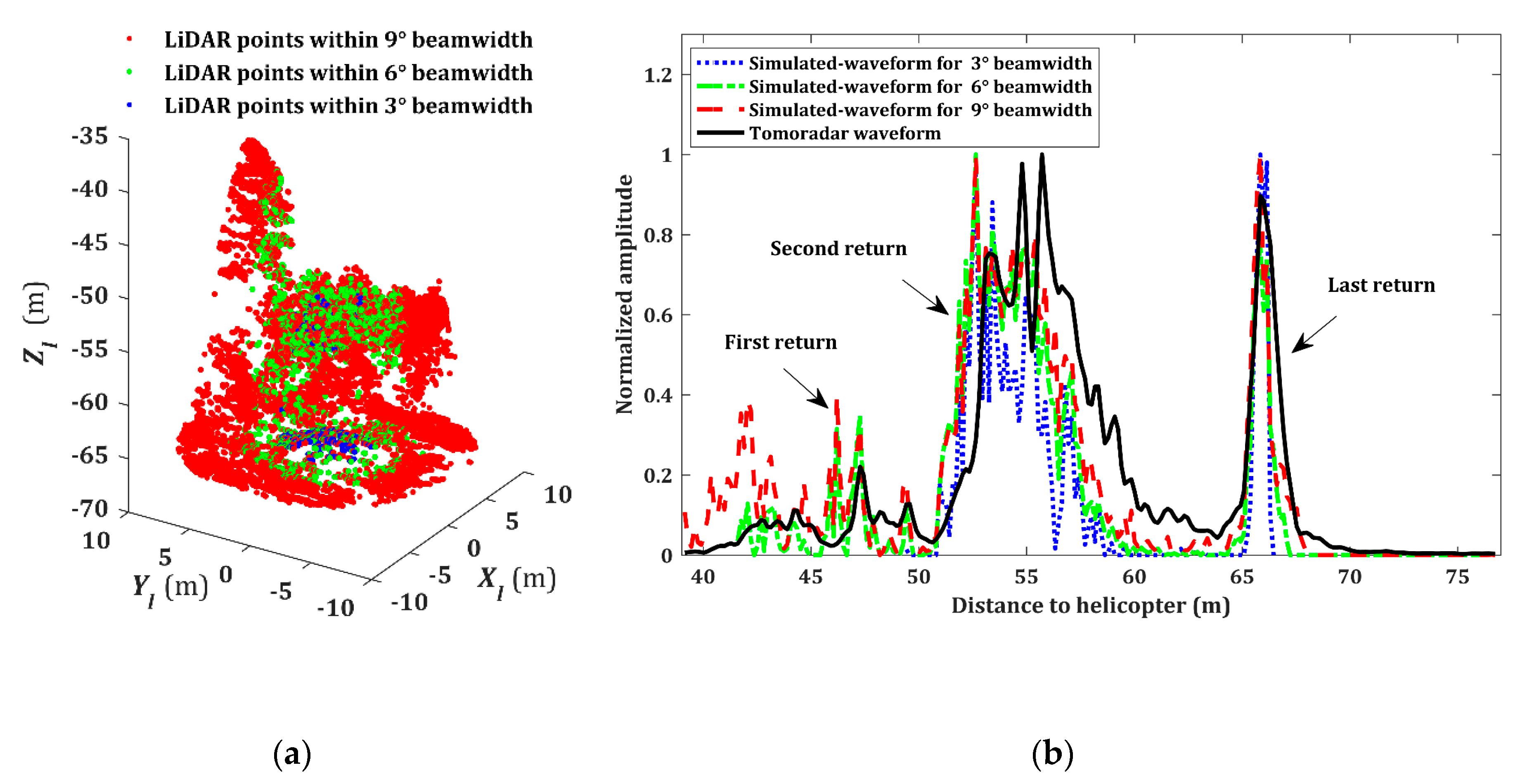
According to the above-mentioned methods, we processed the Tomoradar waveform and generated the simulated-waveforms within Tomoradar cone of 3°, 6°, and 9° for the 6700th Tomoradar measurement in the study area. The corresponding original lidar data and a graphical comparison between Tomoradar waveform and simulated-waveforms are shown in Figure 7.

Figure 7. The lidar points and comparison between Tomoradar waveform and simulated-waveforms within Tomoradar cone of 3°, 6°, and 9° for the 6700th Tomoradar measurement. (a) The original lidar point. (b) Tomoradar waveform and simulated-waveforms. The amplitudes of all waveforms are normalized with the corresponding maximums and described with different colors, respectively.

From the spatial distributions of lidar points in Figure 7a, we discovered that the ground within Tomoradar cone could be roughly considered as a plane with a surface slope of 8.1° and a central distance of 66 m from the Tomoradar reference point. The peak-locations of last returns of all waveforms corresponding to the ground in Figure 7b are approximately close to the central distance, which suggests that the alteration of radar beamwidth could have a negligible impact on extracting the centroid of planar ground. However, the canopy distributions, as shown in Figure 7a are more complicated than those of the ground and considerably fluctuate with radar beamwidth. Hence, the first returns of the simulated-waveforms corresponding to the canopy would change and become much more similar to that of Tomoradar waveform when the radar beamwidth is gradually improved.

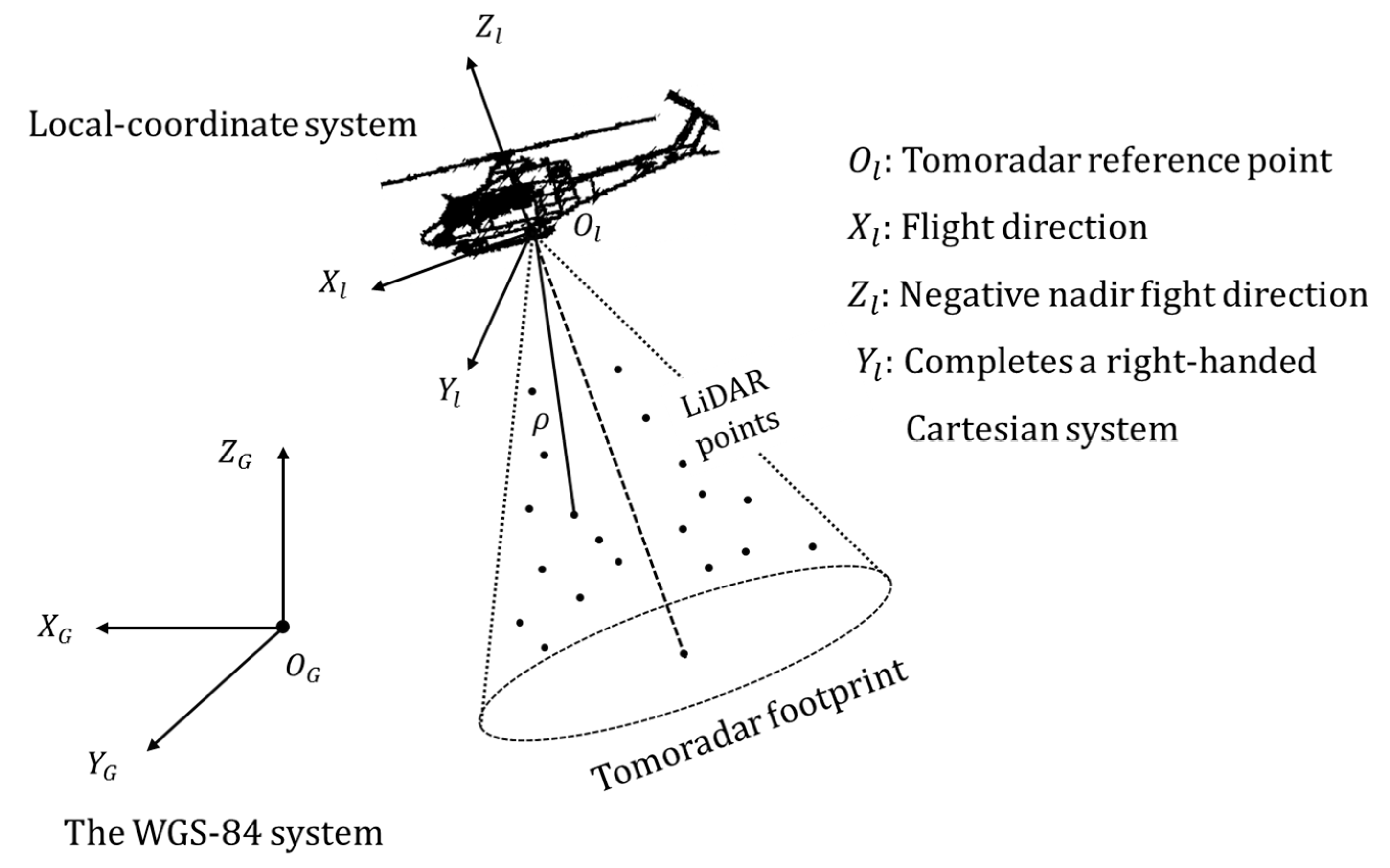
To profoundly explore the reason why radiation energy outside Tomoradar HPBW would contribute to Tomoradar waveform, we firstly transformed each lidar point in Figure 7a from the Cartesian coordinate system $\left(X_l,Y_l,Z_l\right)$ to a new frame $\left(\theta ,\rho \right)$ as

$${\theta }_i=\frac{-Z_{li}}{\sqrt{X_{li}^2+Y_{li}^2}} and {\rho }_i=\sqrt{X_{li}^2+Y_{li}^2+Z_{li}^2}$$

(10)

Then we accumulated the lidar point numbers $N\left(\theta ,\rho \right)$ within a rectangular block with a center of $\left(\theta ,\rho \right)$ and size of $\Delta \theta \times \Delta \rho \left(0.1°\times 0.15\mathrm{m}\right)$, and defined a relative point density as

$$\epsilon \left(\theta ,\rho \right)=N\left(\theta ,\rho \right){\rho }^{-4}$$

(11)

Thus, through introducing Tomoradar antenna pattern in Equation (3), the contribution of lidar points within each block for the simulated-waveform could be roughly expressed by

$$\zeta \left(\theta ,\rho \right)=P_t\left(\theta \right)\epsilon \left(\theta ,\rho \right)$$

(12)

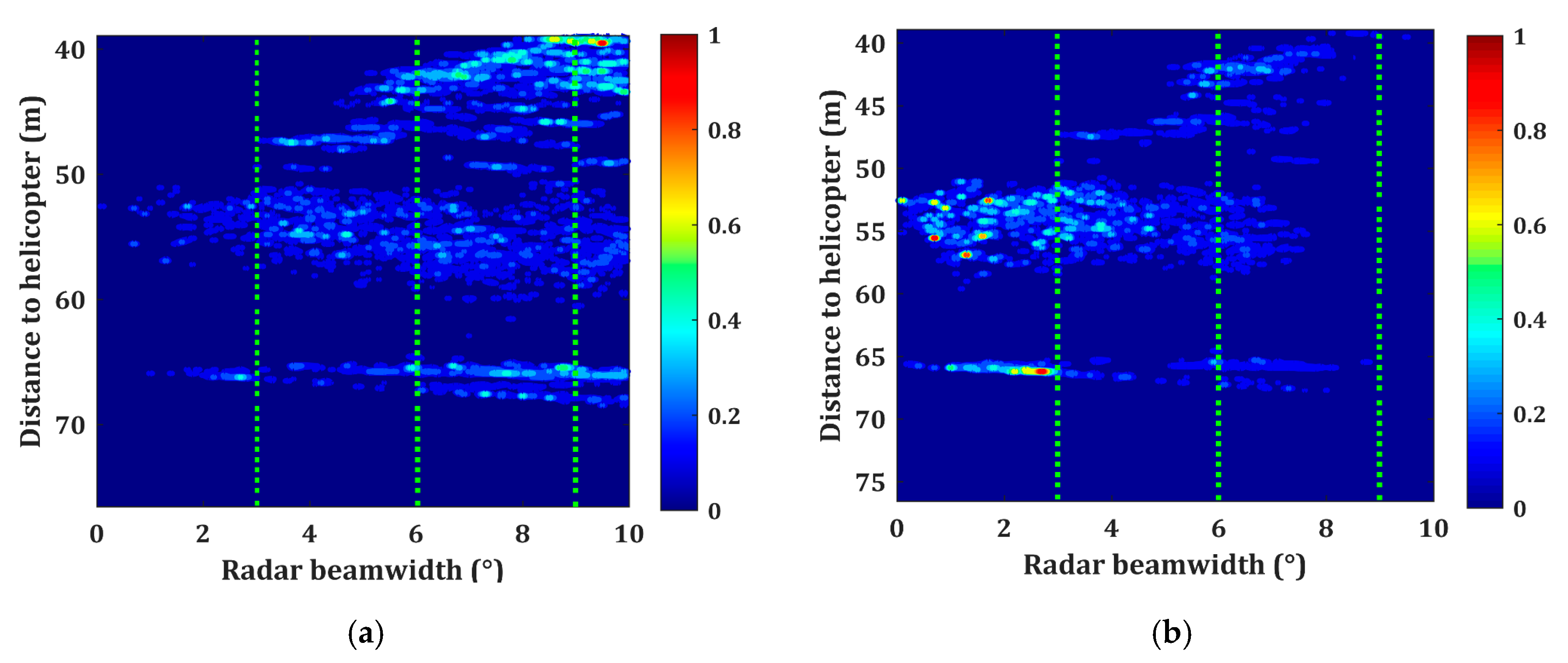
A visual comparison of the relative point density and the contribution of lidar points within each block for radar beamwidths of 3°, 6°, and 9° is illustrated in Figure 8.

Figure 8. (a) The relative point density defined by the 6700th Tomoradar measurement. (b) The contribution of lidar points within each block for the simulated-waveform. All results are normalized by the corresponding maximums, and the locations of three green lines from left to right are 3°, 6°, and 9°.

Observed from Figure 8a, we discovered that three sections of dense lidar points from up to down intensively correspond to the canopy layer, middle layer of vegetation, and the ground, which are primary contributions to the first return, second return, and last return of the simulated waveform in Figure 7b. The location of maximal relative point density is the canopy top with a higher point density and height. However, it may not provide the most significant contribution to the simulated waveform since it is far away from the axial center of Tomoradar and get lesser weight in the Tomoradar antenna pattern. As shown in Figure 8b, the most important contributions of lidar points within each block for the simulated-waveform stem from the middle layer of vegetation and the ground. With the increment of radar beamwidth, the contributions of lidar points at the edge of radar beamwidth are decreased obviously. Therefore, we conclude that there are three factors for determining the contribution of lidar points outside Tomoradar HPBW to Tomoradar waveform: point density, vegetation height, and angular distance to Tomoradar axial center. As for a measured target with higher point density, taller height, and smaller angular distance, its backscattered energy could be bigger than the minimum detection threshold of Tomoradar and be detected by the Tomoradar receiver.

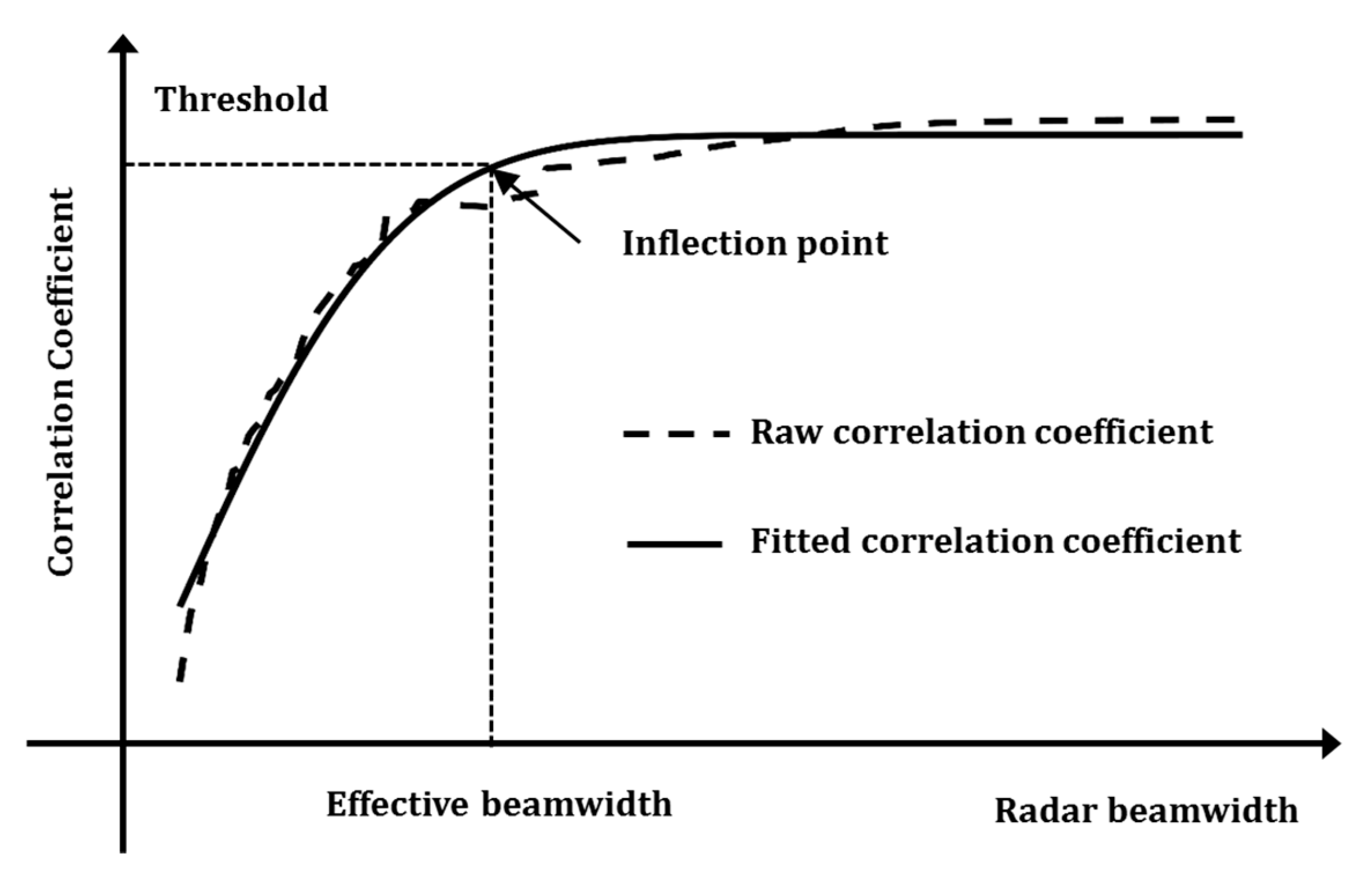
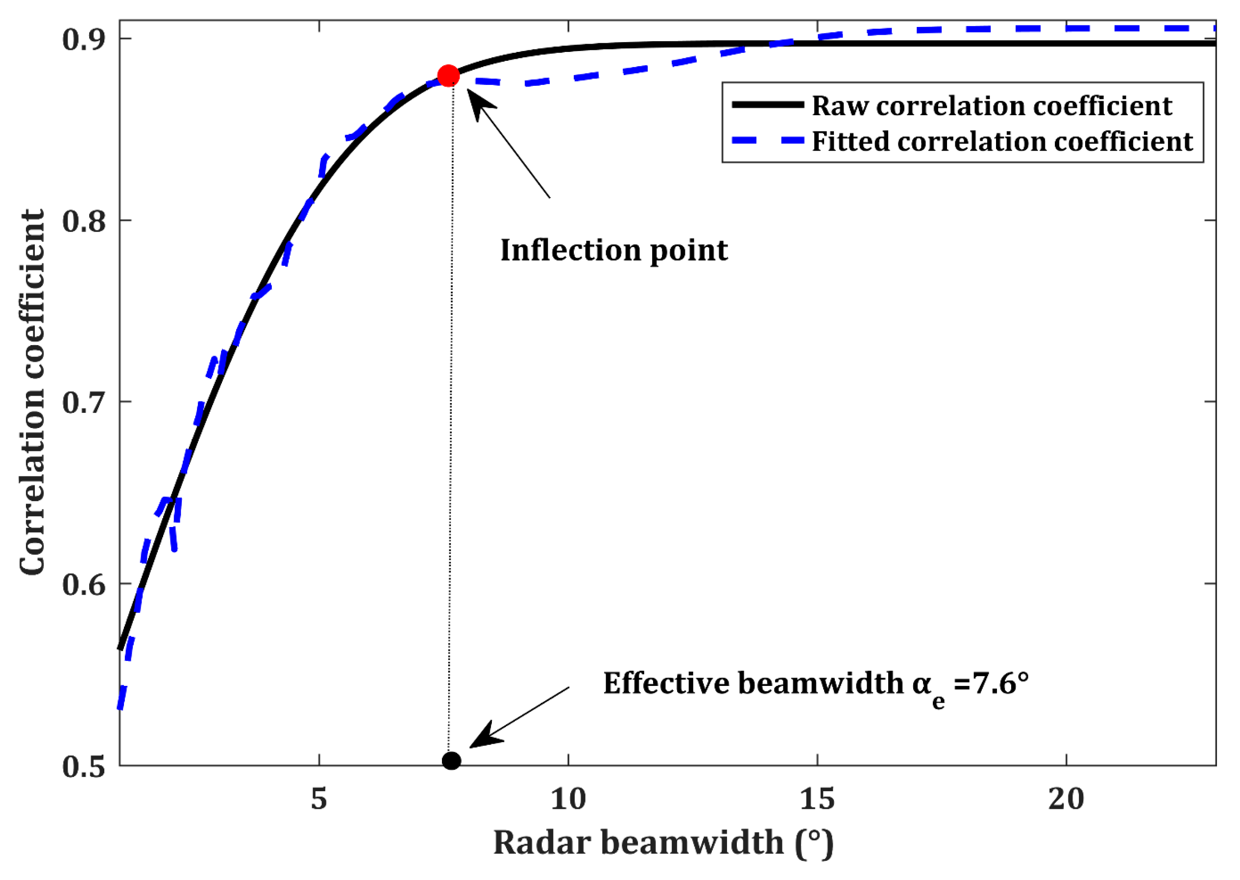
To quantitatively evaluate the similarity between Tomoradar waveforms and simulated-waveforms and find out the effective beamwidth for the 6700th Tomoradar measurement, the correlation coefficients were thoroughly computed for different radar beamwidths and presented in Figure 9.

Figure 9. The distributions of correlation coefficients versus radar beamwidth for the 6700th measurement of Tomoradar. The inflection point is identified at a radar beamwidth of 7.6°.

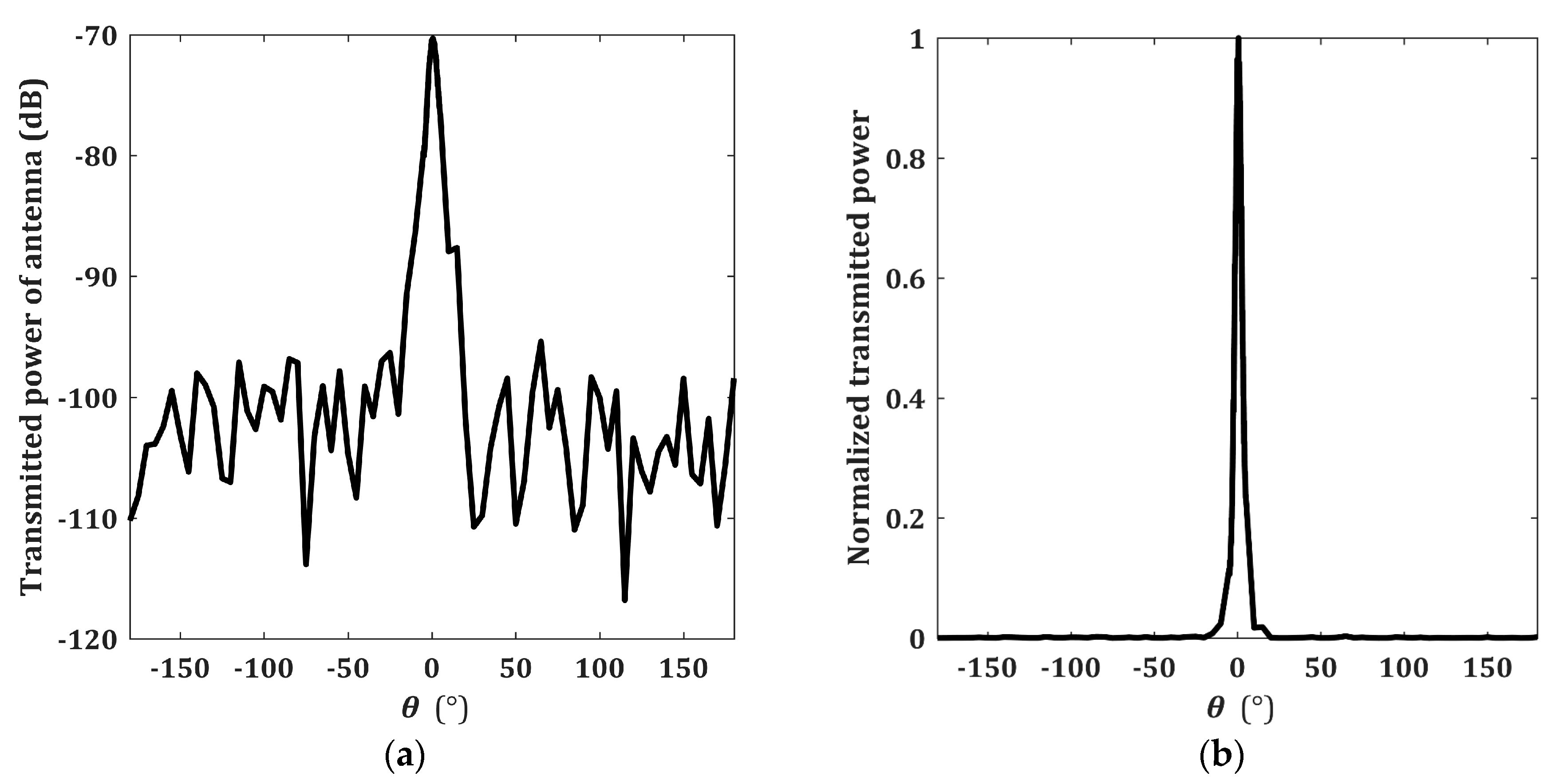
For radar beamwidth of 3°, 6°, and 9°, the correlation coefficients in Figure 9 are 0.71, 0.85, and 0.87, respectively. It implies that the simulated-waveform within a bigger radar beamwidth could have stronger correlation strength with Tomoradar waveform. We sought the inflection point based on the correlation coefficients and found that the effective beamwidth is approaching 7.6°. Combing with the Tomoradar antenna pattern in Figure 4, we discovered that the radiation power at the effective beamwidth was about 9.54% of the maximal radiation power, and a fraction of radiation energy within the effective beamwidth was approximately 90.2% of total radiation energy. The fraction was much greater than the ratio of radiation energy (62.4%) within Tomoradar HPBW. It demonstrates that 27.8% of microwave radiation energy outside Tomoradar HPBW should hit the vegetation and backscatter into the Tomoradar receiver.

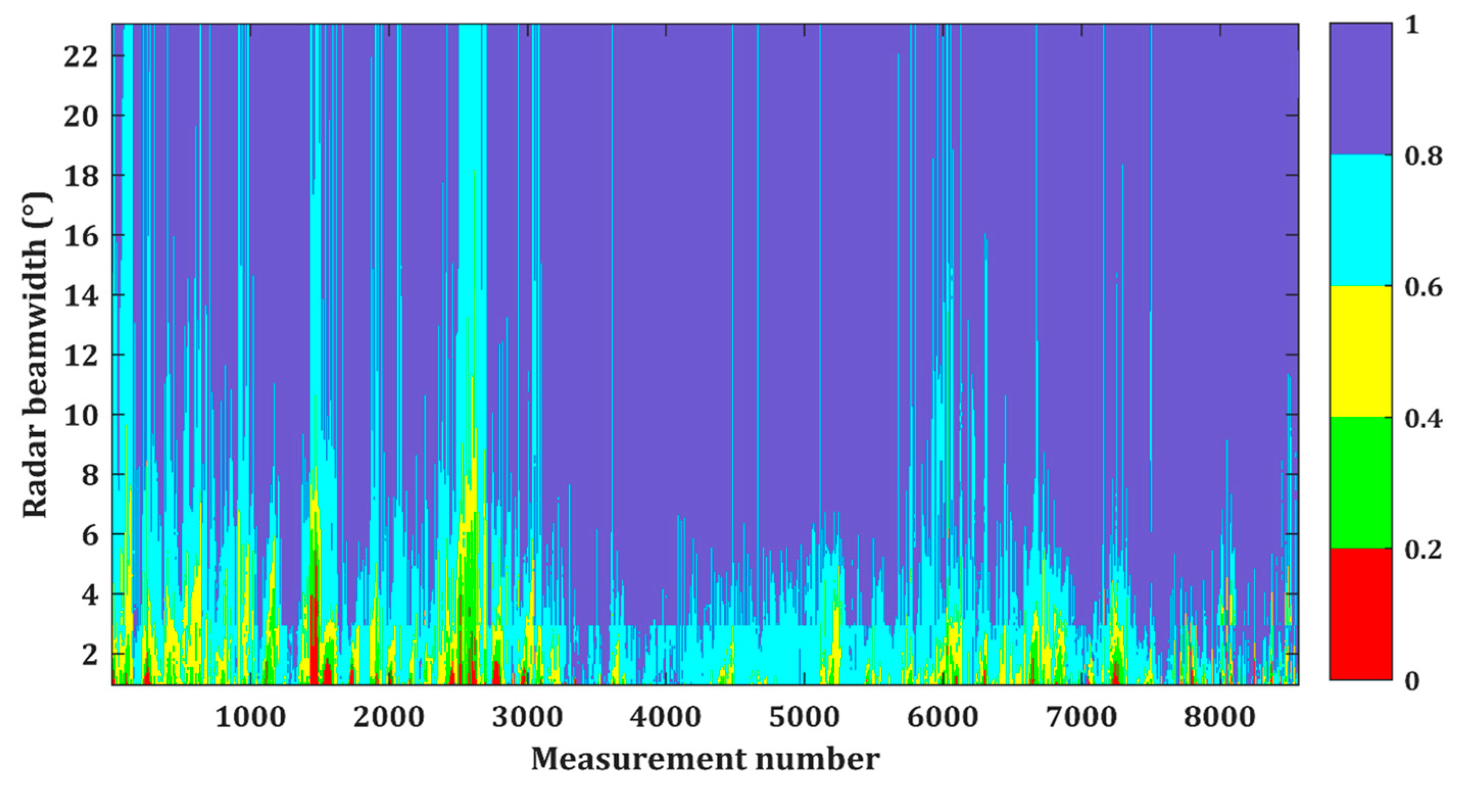
Due to the diverse nature of the vegetation distributions contained in Tomoradar measurement, the simulated-waveform could be distinguished from each other. Thus, the correlation coefficients between Tomoradar waveform and the simulated-waveform would present different regularity. We provide a relationship graph of the correlation coefficients versus radar beamwidth for 8586 Tomoradar measurements, as shown in Figure 10.

Figure 10. The distributions of correlation coefficients between Tomoradar waveforms and simulated-waveforms for 8565 Tomoradar measurements. The correlation coefficients are displayed with a range from 0 to 1 and an interval of 0.2 based on the correlation strength. The correlation strengths are expressed with the colors of red, green, yellow, cyan, and blue from very weak to very strong.

From the distributions of correlation coefficients in Figure 10, we concluded that the correlation coefficients would rise with the growth of radar beamwidth. Based on correlation strength, we partitioned the correlation coefficients into five segments with a range from 0 to 1 and an interval of 0.2. By calculating the numbers within each segment, we obtained the percentiles of all Tomoradar measurement numbers and illustrate some results in Table 1.

Table 1. The percentiles of Tomoradar measurement numbers classified by the correlation strength.

Strength Beamwidth	Very Weak	Weak	Moderate	Strong	Very Strong
3°	0.75	2.96	16.06	45.87	34.36
6°	0	0.72	3.76	26.94	68.58
9°	0	0.01	1.25	17.40	81.34
12°	0	0	0.63	13.24	86.13
15°	0	0	0.31	10.74	88.95
18°	0	0	0.16	9.10	90.74
21°	0	0	0.02	8.30	91.68

In Table 1, about 34.36% of simulated-waveforms have solid correlation strength with the Tomoradar waveforms for radar beamwidth of 3°, but the corresponding fraction would dramatically rise at 68.58% if the radar beamwidth increases to 6°. Indeed, the increasing rate of the percentiles of very strong is slowing down with the further increment of radar beamwidth. When the radar beamwidth is 21°, the correlation coefficient maintains at 91.68%.

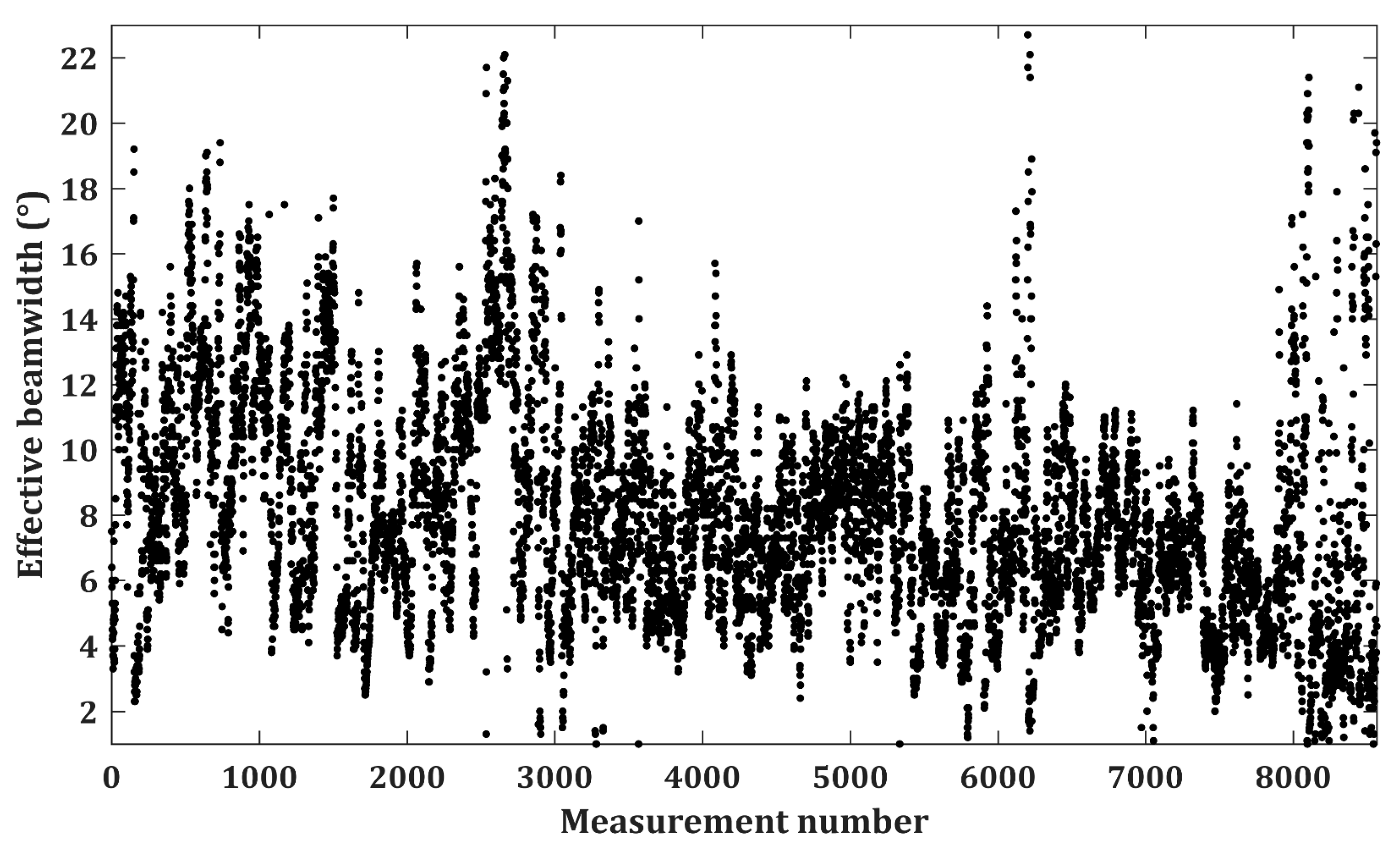
The effective beamwidth for each Tomoradar measurement is strictly dependent on the distributions of the correlation coefficients. That is, the variations of correlation coefficients could influence the determination of the effective beamwidth. Hence, we resolved the corresponding effective beamwidths based on the correlation coefficients in Figure 10 and the extracted model of the effective beamwidth expressed in Equation (9), which are visually presented in Figure 11.

Figure 11. The results of effective beamwidth for 8565 Tomoradar measurements. The dots denote the locations of effective beamwidth for each measurement.

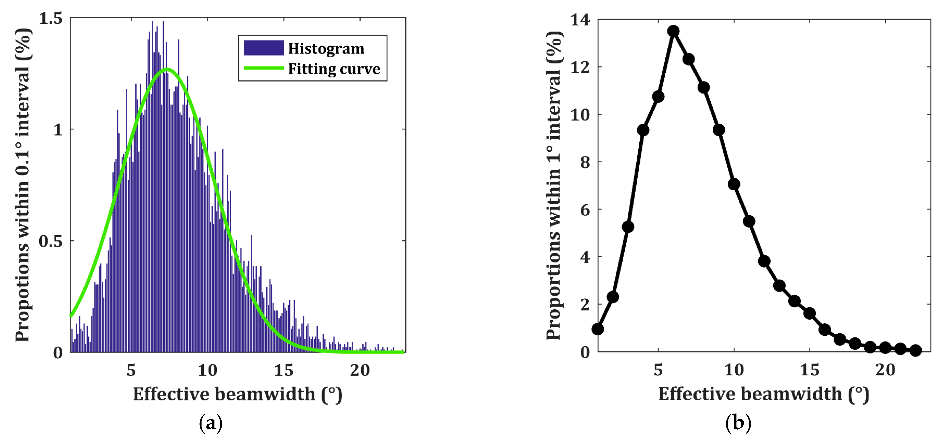
We noticed that the effective beamwidth is variable for each Tomoradar measurement, and most of the effective beamwidths ranged between 3° and 15°. We divided these effective beamwidths into 220 sections within a window from 1° to 23° and an interval of 0.1° and obtained the proportions to total Tomoradar measurements by counting the numbers within each section. A histogram of the proportions is illustrated in Figure 12a.

Figure 12. The distributions of the proportions of effective beamwidth to total Tomoradar measurements within a window from 1° to 23° and each section of different intervals. (a) 0.1° interval; (b) 1° interval.

In Figure 12a, we find a clear normal distribution from the proportions’ histogram with a maximal amplitude of 1.27%, and a peak location of 7.3° and a sigma width of 3.1°. If we change the interval of each section from 0.1° to 1°, then we could acquire the corresponding percentage within every section, as shown in Figure 12b, again, close to normal distribution. The effective beamwidth confined within the windows of (6° and 7°) holds a maximal fraction of 13.5%. Furthermore, 96.43% of the effective beamwidths take values from 3° to 20°, 3.25% of the effective beamwidths are less than 3°, and 0.32% of the effective beamwidths are greater than 20°.

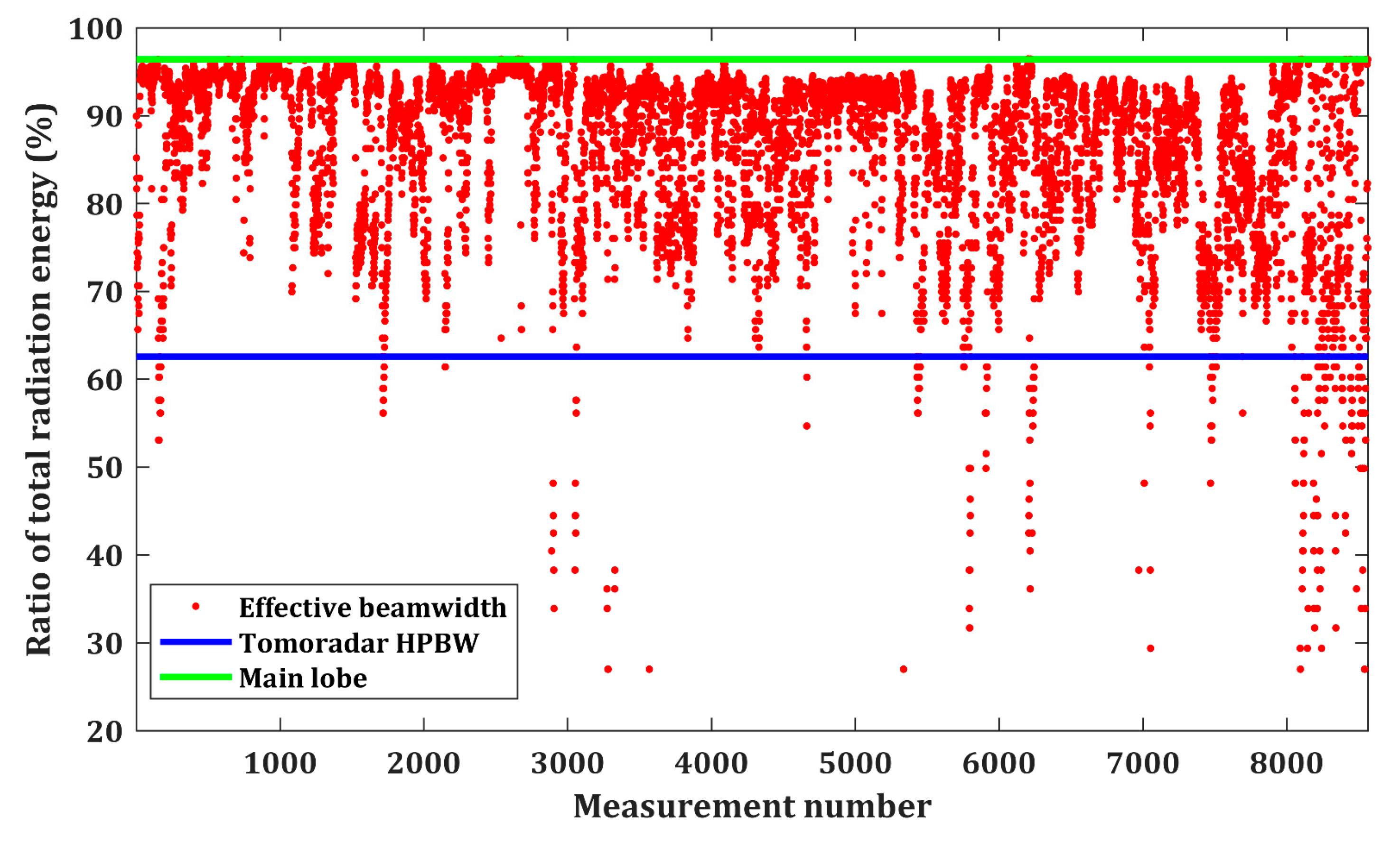
According to the distribution of the effective beamwidth in Figure 11 and Tomoradar antenna pattern in Figure 4, we compute the ratios of radiation energy to total radiation energy within the effective beamwidths as illustrated in Figure 13.

Figure 13. The ratios of radiation energy within the effective beamwidths, main lobe and Tomoradar half-power beamwidth (HPBW), to total radiation energy. The ratio of total radiation energy within Tomoradar HPBW and main lobe are 62.4% and 96.4%, respectively.

From Figure 13, we find the ratios of radiation energy within the effective beamwidths for 96.43% of Tomoradar measurements are ranged between 62.4% and 96.4%. The results demonstrate that it could be inappropriate to utilize Tomoradar HPBW as actual radar beamwidth because more radiation energies are transmitted into the canopy and ground and backscattered into the Tomoradar receiver. The scattered properties of vegetation would determine the radiation energy employed in the investigation of forest and the effective beamwidths.

However, it is impossible to select such variable effective beamwidths as the references for the antenna design and the determination of radar footprint size. Hence, we define an optimal and fixed beamwidth named as average effective beamwidth (AEBW) ${\alpha }_a$ to take the place of Tomoradar HPBW as the following:

$${\alpha }_a=\frac{{{\displaystyle \sum }}_i{\alpha }_e\left(i\right)\gamma \left(i\right)}{{{\displaystyle \sum }}_i\gamma \left(i\right)}$$

(13)

where ${\alpha }_e\left(i\right)$ and $\gamma \left(i\right)$ represent the effective beamwidth and the fraction within each section in Figure 11.

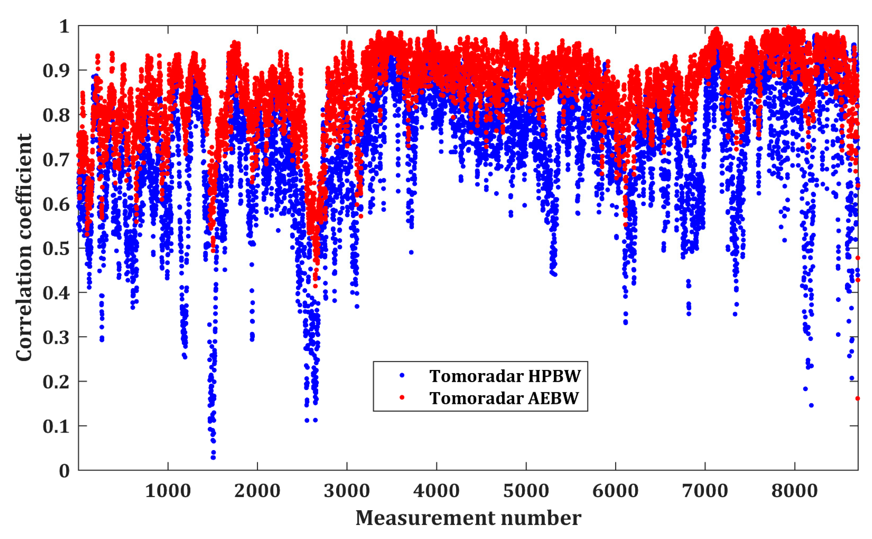
Based on the histogram in Figure 12a, we resolved that Tomoradar AEBW was approximately 8.0° and discovered that the fraction of total transmitted radiation energy should maintain at a level of 91%. Furthermore, we generated the simulated-waveforms from lidar points within a divergence of 8.0° for each Tomoradar measurement and calculated the correlation coefficients between Tomoradar waveform and simulated-waveform. A comparison of the correlation coefficients derived from the simulated-waveforms within Tomoradar HPBW and AEBW is presented in Figure 14.

Figure 14. The distribution of correlation coefficients between Tomoradar waveforms and simulated-waveforms generated from lidar points within Tomoradar HPBW and average effective beamwidth (AEBW).

Observed from Figure 14, the correlation coefficients for Tomoradar AEBW are normally more significant than those for Tomoradar HPBW. About 78.84% of Tomoradar waveforms and simulated-waveforms generated within Tomoradar AEBW have very strong correlation strength. The fraction is much more than that for Tomoradar HPBW described in Table 1. It suggests that Tomoradar waveforms correlate very well with those simulated-waveforms if Tomoradar cone equals to Tomoradar AEBW rather than Tomoradar HPBW.

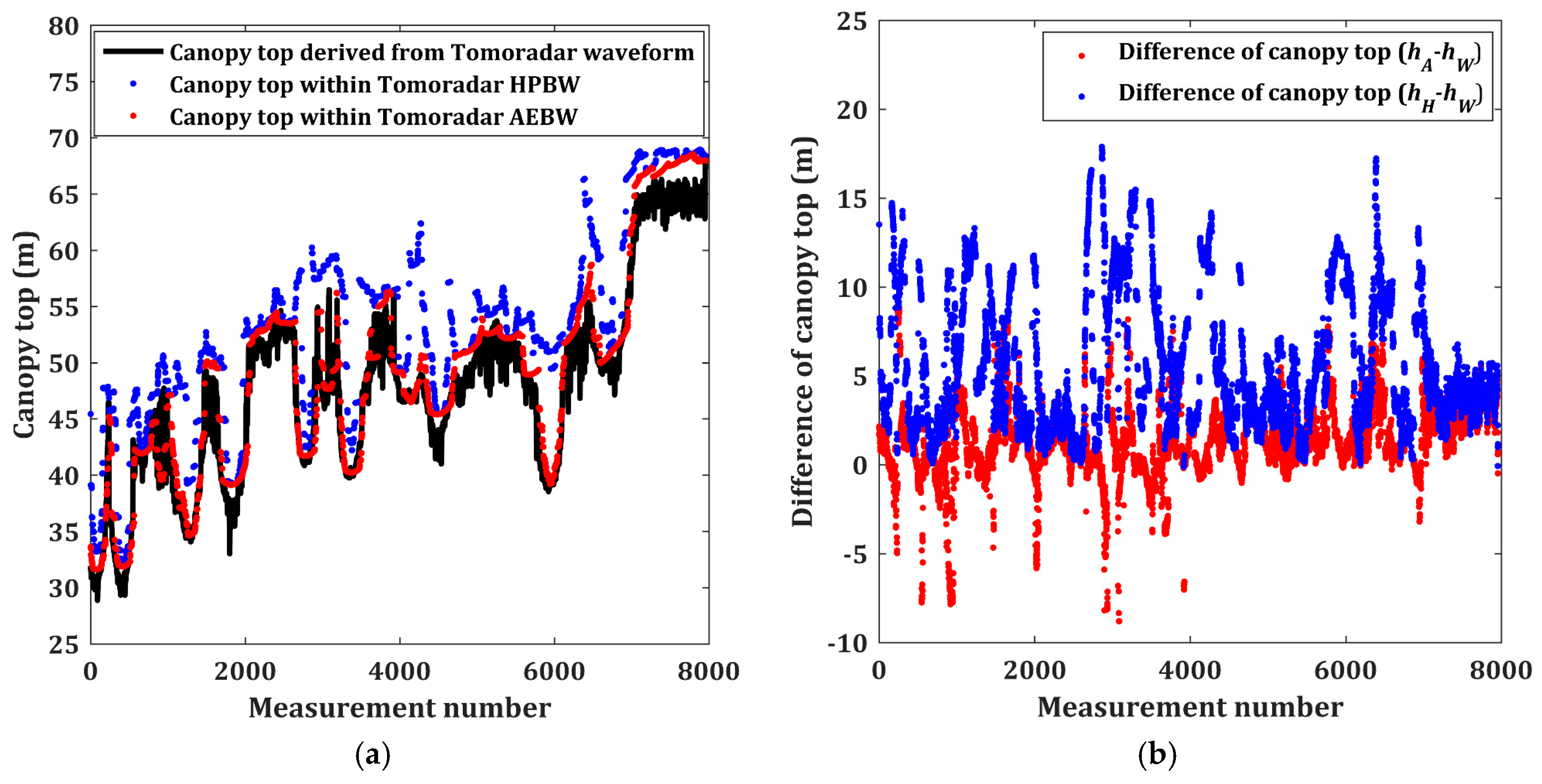
Furthermore, to explore whether Tomoradar AEBW is appropriate in the forest investigation, we extracted the canopy tops from lidar data within the Tomoradar HPBW and AEBW, symbolized with $h_H$ and $h_A$, and compared them with those derived from coincident Tomoradar waveforms, expressed by $h_W$. We designated canopy tops derived from Tomoradar waveforms as references and acquired the difference of canopy tops between them and those within Tomoradar HPBW and AEBW. A graphic description of canopy tops derived from Tomoradar waveforms and lidar data within Tomoradar HPBW and AEBW is shown in Figure 15a. Furthermore, the corresponding differences of canopy tops are presented in Figure 15b.

Figure 15. (a) The canopy tops extracted from Tomoradar waveforms and lidar data within Tomoradar HPBW and AEBW; (b) the differences of the canopy tops. The canopy tops derived from Tomoradar waveforms and lidar data within the Tomoradar HPBW and AEBW are symbolized with $h_W$, $h_H$, and $h_A$, respectively.

We realized that three series of canopy tops present roughly similar fluctuations in Figure 15a. However, the canopy tops extracted from lidar data within Tomoradar AEBW are generally lower than those within Tomoradar HPBW. Moreover, the differences of canopy top derived from Tomoradar AEBW are almost always smaller than those derived from Tomoradar HPBW in Figure 15b. It implies that the canopy tops within Tomoradar AEBW are much closer to those extracted from Tomoradar waveforms than those within Tomoradar HPBW.

To quantitatively assess the differences of the canopy tops extracted from Tomoradar waveforms and lidar data within HPBW and AEBW, we provided three groups of evaluation indexes: correlation coefficients between canopy tops $r\left(h_H, h_W\right)$ and $r\left(h_A, h_W\right)$; (b) standard deviations of the differences of the canopy tops $\delta \left(h_H-h_W\right)$ and $\delta \left(h_A-h_W\right)$; and (c) mean values of the differences of the canopy tops $\tau \left(h_H-h_W\right)$ and $\tau \left(h_A-h_W\right)$. Based on the results in Figure 15, we computed these evaluation indexes, as shown in Table 2.

Table 2. The correlation coefficients of the canopy tops, and the standard deviations and the mean values of the differences of canopy tops derived from Tomoradar waveforms and coincident lidar data within Tomoradar HPBW and AEBW, respectively.

Evaluation Indexes	Results
Correlation coefficients of canopy tops	$r\left(h_H, h_W\right)$	$r\left(h_A, h_W\right)$
	0.89	0.98
Standard deviations of the differences of the canopy tops	$\delta \left(h_H-h_W\right)$	$\delta \left(h_A-h_W\right)$
	3.79 m	1.39 m
Mean values of the differences of the canopy tops	$\tau \left(h_H-h_W\right)$	$\tau \left(h_A-h_W\right)$
	5.55 m	2.04 m

From the results in Table 2, we perceive that the canopy tops derived from lidar data within Tomoradar AEBW correlate very strongly with those derived from Tomoradar waveforms, and the corresponding correlation coefficient is approaching to 1. The standard deviation and mean value of the differences of the canopy top derived from lidar data within HPBW and Tomoradar waveforms individually are 3.79 m and 5.55 m. However, those would become significantly decreased as 2.04 m and 1.39 m if Tomoradar cone is Tomoradar AEBW. These evaluation indexes mean that the canopy tops derived from lidar data within Tomoradar AEBW should be more accurate than those from lidar data within HPBW. That is, Tomoradar AEBW could be more applicable as the actual Tomoradar cone to explain the forest investigation.

4. Conclusions

The radar effective beamwidth determines an actual illuminated area on the measured target rather than traditional HPBW. We proposed a method to determine the effective beamwidth according to the resemblances between radar waveforms and the simulated-waveforms generated from coincident lidar points.

By processing 8565 Tomoradar measurements and corresponding lidar data in a broad and heterogeneous recreation area, we conclude that actual radar effective beamwidths are generally larger than radar HPBW. It suggests that radiation energy outside radar HPBW would commonly transmit into vegetation and backscattered into the radar receiver. Thus, we could determine the radar footprint size depending on not radar HPBW, but the effective beamwidth.

Unfortunately, the effective beamwidth is changeable with the scattering property of vegetation, which makes us unable to designate such unstable beamwidth as radar beamwidth. Therefore, radar AEBW is put forward based on effective beamwidths and corresponding proportions. If we replace radar HPBW with AEBW, we find that the simulated-waveforms correlate better with Tomoradar waveforms and canopy tops derived from lidar data, which are much closer to those extracted from Tomoradar waveforms. These results demonstrate that radar AEBW should be more appropriate in the determination of radar beamwidth. Therefore, as for the forest investigations by profiling radar systems, we suggest that the radar AEBW is a reliable reference to select the region size of validation data.

Due to the diversity of vegetation in the study area, the effective bandwidth of the system does not always follow the AEBW value. By applying the proposed AEBW, the STD of the canopy top difference between LiDAR and Radar decrease from 3.79 m to 1.39 m with an improvement of 63%, and the mean value of the canopy top difference between two active sensors decreases from 5.55 m to 2.04 m with an improvement of 64%. Thus, we consider that the AEBW value can be applied to other scene types of the boreal forest as well for the given Tomoradar.

The uniquity of field test datasets by observing the identical dry boreal forest target with both microwave radar and LiDAR offers an excellent opportunity for us to investigate how the effective bandwidth affect the backscattered signal quantitatively. The Radar return depends on various factors, especially the antenna characteristics. A wider AEBW is determined based on the method proposed in this research to describe the antenna characteristics for more precisely extracting the canopy top of the boreal forest. In addition to the AEBW concept, such an investigation method is also meaningful for other researches on the same topics.

However, radar AEBW could be changed with a variety of radar antenna patterns. So, we suppose that a fraction of total radiation energy within radar AEBW may be a superior index for defining the divergence angle of radar, just like the definition of the lidar footprint based on the percentage of transmitted laser energy. In this paper, we suggest that the fraction is suitable to be 91% in the radar case, which is similar to 86.5% in the lidar case.

References

- Gong, P.; Mei, X.; Biging, G.S.; Zhang, Z. Improvement of an oak canopy model extracted from digital photogrammetry. Photogramm. Eng. Remote Sens. 2002, 68, 919–924. [Google Scholar]
- Karjalainen, M.; Kankare, V.; Vastaranta, M.; Holopainen, M.; Hyyppa, J. Prediction of plot-level forest variables using TerraSAR-X stereo SAR data. Remote Sens. Environ. 2012, 117, 338–347. [Google Scholar] [CrossRef]
- Lovell, J.; Jupp, D.L.; Culvenor, D.S.; Coops, N.C. Using airborne and ground-based ranging lidar to measure canopy structure in Australian forests. Can. J. Remote Sens. 2003, 29, 607–622. [Google Scholar] [CrossRef]
- Hyyppa, J.; Pulliainen, J.; Hallikainen, M.; Saatsi, A. Radar-derived standwise forest inventory. IEEE Trans. Geosci. Remote Sens. 1997, 35, 392–404. [Google Scholar] [CrossRef]
- Tebaldini, S.; Rocca, F. Multibaseline polarimetric SAR tomography of a boreal forest at P and L-bands. IEEE Trans. Geosci. Remote Sens. 2011, 50, 232–246. [Google Scholar] [CrossRef]
- Dinh, H.T.M.; Tebaldini, S.; Rocca, F.; Koleck, T.; Borderies, P.; Albinet, C.; Villard, L.; Hamadi, A.; Le Toan, T. Ground-based array for tomographic imaging of the tropical forest in P-band. IEEE Trans. Geosci. Remote Sens. 2013, 51, 4460–4472. [Google Scholar] [CrossRef]
- Persson, H.J.; Fransson, J.E.S. Forest variable estimation using radargrammetric processing of TerraSAR-X images in boreal forests. Remote Sens. 2014, 6, 2084–2107. [Google Scholar] [CrossRef]
- Hallikainen, M.; Hyyppä, J.; Haapanen, J.; Tares, T.; Ahola, P.; Pulliainen, J.; Toikka, M. A helicopter-borne 8-channel ranging scatterometer for remote sensing, Part 1: System description. IEEE Trans. Geosci. Remote Sens. 1993, 31, 161–169. [Google Scholar] [CrossRef]
- Chen, F.; Hakala, T.; Karjalainen, M.; Feng, Z.; Tang, J.; Litkey, P.; Kukko, A.; Jaakkola, A.; Hyyppä, J. UAV-borne profiling radar for forest research. Remote Sens. 2017, 9, 58. [Google Scholar] [CrossRef]
- Zhou, H.; Chen, F.; Feng, Z.; Puttonen, E.; Hyyppä, J.; Hakala, T.; Karjalainen, M.; Jiang, C.; Pei, L. The comparison of canopy height profiles extracted from Ku-band profile radar waveforms and LiDAR data. Remote Sens. 2018, 10, 701. [Google Scholar] [CrossRef]
- Chen, Y.; Feng, Z.; Li, F.; Zhou, H.; Hakala, T.; Karjalainen, M.; Hyyppä, J. Lidar-aided analysis of boreal forest backscatter at Ku band. Int. J. Appl. Earth Obs. Geoinf. 2020, 91, 102133. [Google Scholar] [CrossRef]
- Feng, Z.; Chen, F.; Hyyppa, J.; Hakala, T.; Zhou, H.; Wang, Y.; Karjalainen, M. Estimating ground level and canopy top elevation with airborne microwave profiling radar. IEEE Trans. Geosci. Remote Sens. 2018, 56, 2283–2294. [Google Scholar] [CrossRef]
- Zhou, H.; Chen, F.; Hyyppa, J.; Feng, Z.; Li, F.; Hakala, T.; Xu, X.; Zhu, X. Estimation of canopy height using an airborne Ku-band frequency-modulated continuous waveform profiling radar. IEEE J. Sel. Top. Appl. Earth Obs. Remote Sens. 2018, 11, 3590–3597. [Google Scholar] [CrossRef]
- Du, K.; Huang, H.; Zhu, Y. Simulation of Ku-band profile radar waveform by extending radiosity applicable to porous individual objects (RAPID2) model. Remote Sens. 2020, 12, 684. [Google Scholar] [CrossRef]
- Panzer, B.; Gomez-Garcia, D.; Leuschen, C.; Paden, J.; Rodriguez-Morales, F.; Patel, A.; Markus, T.; Holt, B.; Gogineni, P. An ultra-wideband, microwave radar for measuring snow thickness on sea ice and mapping near-surface internal layers in polar firn. J. Glaciol. 2013, 59, 244–254. [Google Scholar] [CrossRef]
- Hui, Z.; Yuwei, C.; Yue, M.; Song, L.; Juha, H.; Ling, P. The effect of terrestrial surface slope and roughness on laser footprint geolocation error for spaceborne laser altimeter. Photogramm. Eng. Remote Sens. 2018, 84, 647–656. [Google Scholar] [CrossRef]
- Piermattei, L.; Hollaus, M.; Milenković, M.; Pfeifer, N.; Quast, R.; Chen, F.; Hakala, T.; Karjalainen, M.; Hyyppä, J.; Wagner, W. An analysis of Ku-band profiling radar observations of boreal forest. Remote Sens. 2017, 9, 1252. [Google Scholar] [CrossRef]
- Kwok, R.; Haas, C. Effects of radar sidelobes on snow depth retrievals from Operation IceBridge. J. Glaciol. 2015, 61, 576–584. [Google Scholar] [CrossRef]
- Molchanov, P.; Gupta, S.; Kim, K.; Pulli, K. Short-range FMCW monopulse radar for hand-gesture sensing. In Proceedings of the 2015 IEEE Radar Conference (RadarCon), Johannesburg, South Africa, 27–30 October 2015; Institute of Electrical and Electronics Engineers (IEEE): Johannesburg, South Africa, 2015; pp. 1491–1496. [Google Scholar]
- Vijay, S.K.; Rao, S. Gesture Recognition Using Frequency Modulated Continuous Wave (FMCW) Radar with Low Angle Resolution. U.S. Patent 9,817,109, 14 November 2017. [Google Scholar]
- Hamish, M. Modern Radar Systems; Artech House on Demand: London, UK, 2008; p. 108. ISBN 978-1-59693-242-5. Available online: https://www.radartutorial.eu/06.antennas/an08.en.html (accessed on 8 July 2020).
- Schneider, M. Automotive radar status and trends. In Proceedings of the German Microwave Conference, Ulm, Germany, 5–7 April 2005; pp. 144–147. [Google Scholar]
- Li, L.; Cheng, X. Model to calculate the effect of antenna side lobes in ground-based. Microwave remote sensing of the atmosphere. Int. Soc. Opt. Photonics 1998, 3503, 340–345. [Google Scholar]
- Popescu, S.; Zhao, K.; Neuenschwander, A.; Lin, C. Satellite lidar vs. small footprint airborne lidar: Comparing the accuracy of aboveground biomass estimates and forest structure metrics at footprint level. Remote Sens. Environ. 2011, 115, 2786–2797. [Google Scholar] [CrossRef]
- Parrish, C.E.; Jeong, I.; Nowak, R.D.; Smith, R.B. Empirical comparison of full-waveform lidar algorithms. Photogramm. Eng. Remote Sens. 2011, 77, 825–838. [Google Scholar] [CrossRef]
- Harding, D.; Lefsky, M.; Parker, G.G.; Blair, J. Laser altimeter canopy height profiles: Methods and validation for closed-canopy, broadleaf forests. Remote Sens. Environ. 2001, 76, 283–297. [Google Scholar] [CrossRef]
- Shough, M.L. Radar Detection of Spherical Targets. NARCAP Report. NARCAP Research Associate (United Kingdom), 2009. Available online: http://martinshough.com/aerialphenomena/RCSsphere.pdf (accessed on 8 July 2020).
- Datasheet of PW12000-16000 (12–16 GHz Parabolic Antenna); Chengdu AINFO, Inc.: Chengdu, China, 2020; Available online: http://www.ainfoinc.com.cn/ (accessed on 8 July 2020).
- Benesty, J.; Chen, J.; Huang, Y.; Cohen, I. Pearson correlation coefficient. In Noise Reduction in Speech Processing; Springer: Berlin/Heidelberg, Germany, 2009; pp. 1–4. [Google Scholar]
© 2020 by the authors. Licensee MDPI, Basel, Switzerland. This article is an open access article distributed under the terms and conditions of the Creative Commons Attribution (CC BY) license (http://creativecommons.org/licenses/by/4.0/).