Abstract
Inland aquaculture in Bangladesh has been growing fast in the last decade. The underlying land use/land cover (LULC) change is an important indicator of socioeconomic and food structure change in Bangladesh, and fishpond mapping is essential to understand such LULC change. Previous research often used water indexes (WI), such as Normalized Difference Water Index (NDWI) and Modified Normalized Difference Water Index (MNDWI), to enhance water bodies and use shape-based metrics to assist classification of individual water features, such as coastal aquaculture ponds. However, inland fishponds in Bangladesh are generally extremely small, and little research has investigated mapping of such small water objects without high-resolution images. Thus, this research aimed to bridge the knowledge gap by developing and evaluating an automatic fishpond mapping workflow with Sentinel-2 images that is implemented on Google Earth Engine (GEE) platform. The workflow mainly includes two steps: (1) the spectral filtering phase that uses a pixel selection technique and an image segmentation method to automatically identify all-year-inundated water bodies and (2) spatial filtering phase to further classify all-year-inundated water bodies into fishponds and non-fishponds using object-based features (OBF). To evaluate the performance of the workflow, we conducted a case study in the Singra Upazila of Bangladesh, and our method can efficiently map inland fishponds with a precision score of 0.788. Our results also show that the pixel selection technique is essential in identifying inland fishponds that are generally small. As the workflow is implemented on GEE, it can be conveniently applied to other regions.
1. Introduction
Fishery in Bangladesh has been increasing rapidly in the last few decades as a major source of food and economic growth [1]. According to the International Food Policy Research Institute (IFPRI), the fish farming market has grown 25 times in all aspects of the aquaculture industry in the last three decades. Shahin et al. [2] also reported that the total fish production increased from 4.99 Lac MT (100,000 metric tons) in 1998–1999 to 14.47 Lac MT in 2012–2013. Though rice is still the major food source for Bangladesh, the booming aquaculture is bringing diversity to the dietary structure of people in Bangladesh and gradually improving people’s health conditions [3]. However, the growing aquaculture puts pressure on already limited croplands. In recent years, a great portion of croplands in Bangladesh has been gradually transforming to other land use types, such as fishponds, brickyards, and residential area [1,4]. While Bangladesh Statistical Bureau (BSB) publishes statistical yearbooks every year, it lacks information of the spatial distribution of the land use changes. Such information can better help decision-makers make land use policies for better resource distributions. With earth observation (EO) data, especially newly published Sentinel-2 Multispectral Instrument (MSI) 10 m resolution images, mapping and monitoring individual fishponds become feasible. In addition, the advent of Google Earth Engine (GEE) significantly reduced the workload and time of remote sensing data preprocessing, analysis, and visualization [5]. Thus, it is important to investigate the potential of using Sentinel-2 images and GEE platform for fast, timely mapping of inland fishponds in Bangladesh.
There are many research works focus on mapping aquaculture ponds in coastal area of South Asia [6,7,8]. However, inland fishponds differ from coastal aquaculture ponds in that inland fishponds are typically owned by individual families, which means they can have arbitrary shape and size and are not necessarily well-aligned as many coastal aquaculture ponds do. Some key features of fishponds in Bangladesh are that:
- (1)
- they are usually filled with water all year round,
- (2)
- they are small, and
- (3)
- like many other man-made objects, they have regular boundaries and simple shapes, such as rectangles.
To address feature (1), multi-temporal and multi-spectral remote sensing images should be used. High-resolution images are the most suitable data to address feature (2). Specifically, based on the research conducted by Belton and Azad [9], the average size of homestead fishponds in Bangladesh is between 0.08 to 0.1 ha, the median value can be even less due to the skewness towards a few large fishponds, which can go up to over 100 ha each. Fishponds with such small size are challenging to detect on medium-resolution (2–30 m) remote sensing images, and it is almost not feasible to do with low-resolution (>30 m) images. However, high-resolution images, such as SPOT (Satellite Pour l’Observation de la Terre) and IKONOS, are usually not available free of charge. Sentinel-2 MSI L1C data has become increasingly popular for land use and land cover (LULC) mapping in recent years mainly because of its finer spatial resolution (10 m) and temporal resolution (10 days before Sentinel-2B launches and 5 days after) [10,11,12]. The significant improvement of both spatial resolution and temporal resolution offered great potentials of improving existing applications and enabling new missions, such as object detections [11]. Therefore, this research uses Sentinel-2 MSI L1C data for fishpond mapping.
Water indexes (WI), such as Normalized Difference Water Index (NDWI) [13], Modified Normalized Difference Water Index (MNDWI) [14], and Automated Water Extraction Index (AWEI) [15], have been developed to enhance water features on multi-spectral images. Most of the WIs utilize low reflectance of water in near-infrared (NIR) and shortwave-infrared (SWIR) spectrum [12,13,16,17]. NDWI takes the difference between the green band and the NIR band, which produce positive values for water and negative values for other LULC types [13]. To address false positives from built-up using NDWI, Xu introduced MNDWI, which is calculated with green and SWIR bands [14]. Previous research reported that MNDWI generally has a more stable threshold than NDWI [16,18,19]. Aside from the NDWI and MNDWI that use 2 bands to compute, AWEI uses 5 bands to compute, and it aims to reduce false positives coming from shadow pixels [15]. The AWEI consists of two formulas, AWEIsh for areas that are contaminated by shadows, and AWEInsh for areas that are not [20]. Feyisa et al. reported that AWEI has much more stable optimal thresholds than MNDWI [15].
To address feature (3), shape-based metrics can be used to help characterize fishponds and non-fishponds. Object-based features (OBF), also referred to as geometrical features in Reference [21] and as shape metric in Reference [22], have been used in previous research as ancillary features in object-based image analysis. In a research conducted by van der Werff and van der Meer [23], shape measures were extracted from Landsat image objects and were used to help classify spectrally identical objects, e.g., rivers and different shapes of lakes. Jiao et al. [22] used 10 shape metrics to classify 8 LULC classes, including rivers and ponds, on SPOT-5 images. Their results showed that such metrics can well characterize all LULC classes quantitatively. For water features specifically, they characterized rivers as elongated, concave, and complex, while ponds were round, rectangular, convex, and simple [22]. Both research works reported that OBFs significantly improved classification accuracy especially when objects are spectrally similar. However, previous research typically works with high-resolution images or objects that are large compared to the pixel sizes, so it is unclear how such OBFs will help with classifying small objects on relatively coarse resolution images.
Therefore, to investigate the performance of using WI and OBFs for inland fishpond mapping, this research aimed to develop a GEE-based workflow that incorporates spectral-based filtering with multiple WIs and spatial-based filtering with OBFs for fishpond mapping. To our knowledge, this is the first study that presents fully automated workflow for inland fishpond mapping. A case study in the Singra Upazila of Bangladesh was conducted to evaluate the performance of the workflow.
2. Study Area and Dataset
The study area of the case study we chose is the Singra Upazila (24°30′ N 89°08′ E) in Bangladesh, as shown in Figure 1. It is a sub-district of Natore district in Northern Bangladesh that consists of 13 unions, namely Chamari, Chaugram, Chhatar Dighi, Dahia, Hatiandaha, Italy, Kalam, Lalore, Ramananda Khajura, Sherkole, Singra Paurashava, Sukash, and Tajpur. More than three hundred thousand people live in around 530 sq. km areas with a density of 607 persons per sq. km. Around 80% of people in this area are engaged with agriculture, more specifically rice crop farming. Since this area is located within one of the largest flood plains of the country, most of the agricultural fields are flooded in the rainy season every year. A recent trend of land use change from crop fields to fishponds has been found in this area because of the larger profit of fish culturing than growing rice.
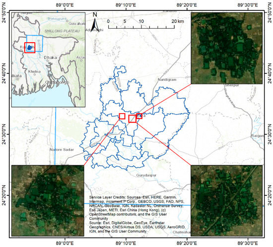
Figure 1.
Study area. Upper left: location of the study area in Bangladesh. Upper right, lower left, and lower right: example fishponds within the study area. The blue boundary on the overview map and the main map shows the footprint of the Sentinel-2 image used in this study.
In addition to the Singra upazila, where fishponds are located at, we also chose a subarea in Tibetan Plateau (upper-left corner: 84°52′ N 31°49′ E; lower-right corner: 87°49′ N 29°55′ E) to select non-fishpond water features to train a classifier for fishpond classification. Tibetan Plateau has an average elevation of over 4000 m, and the plateau is rich of water resources with over 1500 lakes scattered on the plateau [24]. There are three reasons why we selected a region on Tibetan Plateau for non-fishpond sample selection. First, Bangladesh does not have many permanent water bodies for classification. Second, Tibetan Plateau has over 1200 lakes larger than 1 sq. km, as well as multiple river streams [25]. Third, Tibetan Plateau has over 4000 m average altitude, which significantly limited human activities, such as fishery. Therefore, there are rarely any artificial water features in the area.
The dataset used in this study is the Sentinel-2 MSI Level-1C product hosted on GEE. It was preprocessed by radiometric and geometric corrections. As a result, the Sentinel-2 Level-1C is a Top-of-Atmosphere (TOA) reflectance dataset that consists of 100 km by 100 km image tiles projected in UTM/WGS84. The Multi-spectral instrument (MSI) sensors onboard Sentinel-2 satellites collect images with 13 spectral bands in the visible/near-infrared (VNIR) and SWIR spectrums, and the spatial resolutions of the spectral bands vary from 10 m to 60 m. The bands that were used in this study are listed in Table 1. The Military Grid Reference System (MGRS) tile number for all images used in this study is 45RYH.

Table 1.
The Sentinel-2 Level-1C bands used in this study.
3. Methodology
The methodology we used can be divided into two parts, (1) spectral filtering and (2) spatial filtering. The spectral filtering phase conducts image segmentation on multi-temporal Sentinel-2 images to detect all-year-inundated water features. The spatial filtering phase further classifies water features into fishpond class and non-fishpond class based on OBFs. A diagram of the workflow is shown in Figure 2. Details are discussed in the following subsections.
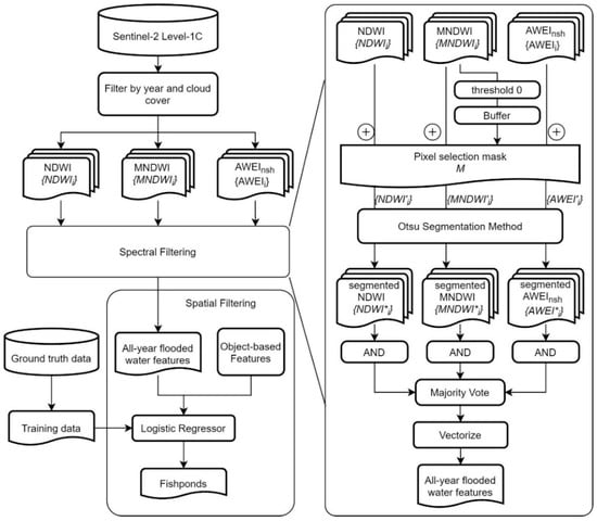
Figure 2.
Proposed workflow.
3.1. Data Preprocessing
Multi-temporal images are first prepared for the detection of all-year-inundated water features rather than seasonal water features, such as rice paddy and flooding [12,26,27]. Specifically, all Sentinel-2 Level-1C images with less than 10% cloud cover in 2016 were collected. The images that satisfy the selection criteria are the four images in 2016 on January 16th, January 31st, April 30th, and October 17th. Here, we denote the image collection as , where n is the total number of images. Note that, due to extremely high cloud cover during monsoon seasons, no images are available between May and September.
Three WIs, i.e., NDWI, MNDWI, and AWEInsh, were calculated for each selected image . We denote the three WI image collections as . AWEIsh was not used because most fishponds are in rural areas where the noise from shadow is minimal. For the convenience of notation, the rest of the paper use AWEI to refer to the AWEInsh. Table 2 summarizes the aforementioned three WIs. Figure 3. shows the WI images for a selected area. As shown in the figure, fishponds show consistently high WI values, while rice paddy and floods show seasonal variations.
Table 2.
Equations of the three water indexes (WIs) used in this study. in the equations represents Top-of-Atmosphere (TOA) reflectance of corresponding Sentinel-2 bands, e.g., is the TOA value of Sentinel-2 near-infrared band.
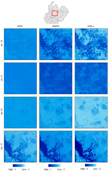
Figure 3.
WI images of four dates in 2016 in an example area within the study area. Value ranges for Normalized Difference Water Index (NDWI) and Modified Normalized Difference Water Index (MNDWI) are −1 to 1 and −2 to 2 for AWEInsh. No color stretches are applied. Higher WI values are shown in darker shade of blue.
3.2. Spectral Filtering
The spectral filtering phase transforms input multi-temporal Sentinel-2 images to a single mask which mask out all pixels that are not inundated all-year-round. The spectral filtering phase include two steps, a pixel selection step and an image segmentation step, and details are discussed in the following two subsections.
3.2.1. Pixel Selection Technique
Many threshold-based image segmentation methods favor bimodal histograms because thresholds can be easily found in the valley of two peaks without much uncertainty [28,29]. Therefore, it is reasonable to do a pre-masking to reduce the number of non-water pixels in threshold selection for fishponds that are typically small and scarcely scattered in a large area. To achieve that, we adapted and modified a technique that was used in previous research [28,29,30,31]. Specifically, a preliminary thresholding step was conducted using a forgiving threshold to loosely identify water features, and then buffers are generated around the water features to include some but not all non-water pixels. Detailed steps of this approach are described below:
- (a)
- An empirical threshold 0 was used for all multi-temporal MNDWI images, denoted as , to loosely classify water features.
- (b)
- All classified MNDWI images were combined by inserting logical operator AND between images to get a single layer mask, denoted as , where pixel value 1 represents all-year-inundated water features.
- (c)
- The mask from (b) was then vectorized by connecting neighboring same-value pixels.
- (d)
- Buffer polygons were generated from each water feature. The buffer distance was set to 5 pixels.
- (e)
- The buffered polygons were then rasterized as a binary mask image for pixel selection.
In the above steps, step (a) and (b) were to identify all-year-inundated water features, step (c) and (d) aimed to generate a pixel selection mask that includes only a portion of all pixels, the masking operation is illustrated as follows:
Masked WI image collections were then used as input to the image segmentation step that is discussed in the following subsection.
3.2.2. Image Segmentation
The threshold selection of WIs is the key factor of accurately mapping water on multispectral images [11,19]. An empirical threshold 0 is chosen by default for many WIs [13,16,32]. However, due to mixed pixels of water and other land cover types, the optimal WI thresholds usually depend highly on the scene and locations [15]. Therefore, previous research uses dynamic thresholds to adapt to varying situations. Among many automatic thresholding algorithms, the Otsu method, which is an automatic grey-level image segmentation algorithm that iteratively finds the optimal threshold that maximizes inter-class variance [33], is widely used for water body mapping [10,12,30,34,35,36]. In research conducted by Yin et al. [37], the Otsu method achieves the best performance among 8 other automatic thresholding methods, and its performance is on par with support vector machine (SVM) and optimal thresholds. Thus, the Otsu method is chosen as the segmentation algorithm in the workflow.
The Otsu method takes in masked WI image collections and produces thresholds for all images within each collection . The thresholds were then used to segment original WI images into binary classes, the segmented image collections are denoted as . Then, each segmented WI image collection, i.e., is self-combined by inserting logical operator AND between pairs of images, which produces single-layer consensus results where pixel value 1 represents all-year-inundated water features. With all three single-layer results, the final all-year-inundated water feature classification result was generated by conducting majority vote among all three layers, pixels that get more than 1 vote will be labeled as 1, while the rest are labeled 0.
3.3. Spatial Filtering
The spatial filtering phase follows the spectral filtering phase, and it transforms the binary mask image from spectral filtering phase to a feature collection. The feature collection contains all polygons that are classified as fishponds. The spatial filtering phase first vectorizes the binary mask image from spectral filtering phase by connecting neighboring homogeneous pixels, which groups connecting pixels into objects. For each water feature vector object, several OBFs were computed using its perimeter, area, and the perimeter and area of its convex hull. A trained machine learning model is then used to classify all water features into fishponds and non-fishponds using OBFs as features.
3.3.1. Object-Based features
OBFs are representations of geometries which are usually used to describe spatial characteristics of geometries [38] and used as auxiliary features in object detection [39,40]. OBFs are effective in measuring the shape complexity of polygons [41,42]. In this research, we mainly used OBFs that can be calculated with perimeters and the area of the target object and its convex hull because the workflow is implemented on GEE, which has limited functionalities for object-based analysis. Table 3 summarizes the OBFs that we used in this research.
Table 3.
Object-based features (OBFs) that were used in this research ( and : area and perimeter of the features; and : area and perimeter of the convex hull of the features).
IPQ, also known as FORM (form factors), SI (shape index), is a widely used measurement of shape compactness [21,22,23,41,43]. The IPQ measures similarities between an object and the most compact shape, i.e., circles, and it is scale-invariant. The range of IPQ is 0 to 1 with 1 being full circles and 0 being infinitely complex shapes. SOLI (Solidity) measures the extent to which an object is convex or concave [22]. The range of solidity is between 0 and 1 with 1 being completely convex. PFD (patch fractal dimensions) or simply fractal dimension is another widely used measurement of shape complexity [22,41]. In the equation in Table 3, the perimeter of the geometry is divided by 4, which accounts for the raster bias in perimeters. PFD values are close to 1 when geometry shapes are simple, e.g., squares and rectangles. It approaches 2 when shapes become complex. CONV (convexity) is a measurement of the convexity of a geometry similar to SOLI. The value range for CONV is between 0 and 1 with 1 being convex shapes, and values less than 1 for objects with irregular boundaries [23]. Lastly, SqP (Square pixel metric) is a very similar metric with IPQ, and it measures the shape convexity of an object. SqP is 0 for a square and approaches 1 as the shape becomes more complex [44].
3.3.2. Ground Truth Sample Collection
To classify fishponds based on OBFs, we first manually digitized fishponds in randomly selected 7 of 13 unions that are within the Singra Upazila as ground truth data. Of the 7 unions, 3 randomly selected unions (Chhatar Dighi, Kalam, and Ramananda Khajura) were then used to derive positive samples for training purposes, and the remaining 4 unions (Chaugram, Italy, Sherkole, and Singra Paurashava) were used to evaluate the method. Note that positive samples were simply a subset of water feature objects generated from the spectral filtering process that intersects with ground truth fishpond polygons. The reason why manually digitized ground truth polygons were not used directly for training purpose is that manually digitized polygons have over-simplified boundaries, which cannot represent the true shapes of water feature polygons generated by segmenting remote sensing images.
In addition to positive samples, i.e., fishponds, negative samples of non-fishpond water features were collected using the Joint Research Centre (JRC) Yearly Water Classification dataset [45]. The JRC dataset provides 30-m resolution images of seasonal and permanent water features every year since 1984. Permanent water features from the region on Tibetan Plateau that was introduced in Section 2 were extracted as negative samples.
The JRC dataset is a 30-m resolution dataset, which is 9 times the resolution of Sentinel-2 MSI in terms of the pixel area. As a result, same-area objects on the JRC layer should have much simpler boundaries than on Sentinel-2 images. More specifically, same-shape objects on Landsat images should be 9 times as large as they are on Sentinel-2 images. According to Belton and Azad [9], fishponds in Bangladesh are typically within a range of 0.02 ha and 100 ha. Therefore, to compensate for the simplification of shapes caused by the difference of spatial resolutions between the JRC dataset and Sentinel-2 images, water features that are 9 times the size of fishponds, i.e., water features that are within 0.18 ha to 900 ha in the region were selected. The geographic area used to select training samples is shown in Figure 4. In total, 708 positive samples and 1086 negative samples were used in the training process.
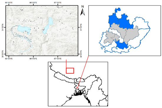
Figure 4.
Locations of region used to select training and test samples. Upper left: the region on Tibetan Plateau for selecting negative samples. Upper right: blue unions are for training positive samples; grey unions are for testing samples.
3.3.3. Fishpond Classification
The last step of the workflow is to classify water feature polygons based on their OBF values. We compared two widely used classification models, i.e., the Logistic Regression (LR) model and Decision Tree (DT) model that are easy to implement on GEE and easy to interpret. The model with better performance was then selected and implemented as the classifier in the workflow.
DT is a widely used classifier that recursively partitions feature space to form purer small subspaces [46]. DTs are easy to interpret as decision rules are no more than a few chained thresholds on features. Moreover, DT provides feature importance score that can help with feature selection. LR is a widely used binary classifier. It has a solid theoretical background, and it is very fast to run due to its simplicity [47]. It is also very simple to implement. A major reason of choosing LR and DT in this experiment is that it is trivial to transplant the fitted models to GEE because LR can be implemented as thresholding the weighted sum of all feature values, and DT can be implemented as a set of nested IF-ELSE statements.
3.4. Accuracy Assessment
As mentioned in the previous section, we manually digitized fishponds in our test site for 2016, which is the study year of this research, based on Google Earth historical satellite images. Among all digitized fishponds, a small portion was used for training purpose, and the rest are used as testing samples. As we only have positive samples for testing, the evaluation was then based on the ‘hit’ rate. Specifically, an identified fishpond is considered correctly identified if its centroid is within a ground truth polygon, hence a ‘hit’. A partial confusion matrix can be constructed with (1) TP (true positives), which is the number of ‘hits’, (2) FP (false positive), which is the number of all classified fishponds minus the number of ‘hits’, and (3) FN (false negative), which is the number of all ground truth polygons minus the number of ‘hits’. Precision, Recall, and F1 score can then be calculated. The equations to calculate the evaluation metrics were shown in Equation (1) to (3):
4. Results
4.1. Fishpond Classification Results
An LR classifier and a DT classifier were built using training samples. The classifiers were built and validated using a 5-fold cross-validation scheme. Specifically, the training dataset was split into 5 parts, and, for each iteration, 4 of them were used as training set, and the last one was used as validation set. To avoid building an overcomplicated DT classifier such that it is inconvenient to transplant the model on GEE and also to reduce overfitting, we limited the max depth of the DT to 3. Moreover, to further reduce overfitting, the minimum samples in the leaf node is set to 50. Table 4 shows the cross-validation results for both LR and DT. From Table 4 we can see that DT generally performs slightly better than LR as the average training and validation scores of DT are both around 3–4% higher than LR. The training score and validation scores are close, which means the models are not overfitting. Table 5 shows the weights of the trained LR model. Figure 5 illustrates the tree structure of the trained DT model. From Figure 5, we can see that the leaf nodes of the left branch of the tree are all fishpond class; thus, the tree can be simplified by representing all leaf nodes on the left branch as one node with splitting criteria , which simplified the transplantation of the model on GEE.
Table 4.
Five-fold cross validation score of implemented Logistic Regression (LR) and DT models.
Table 5.
Coefficients of OBFs using the optimal LR model.
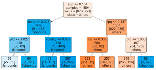
Figure 5.
Decision Tree (DT) tree structure (blue nodes indicate fishpond class, and orange nodes indicate other water types).
Figure 6 shows fishpond classification results of three example subareas. The first subarea (left column) is a small village that contains densely located fishponds. By comparing the AWEI image in Figure 6a and the ground truth layer in Figure 6d, we can see that the majority of fishpond boundaries are visually clear to identify, while some fishponds are too close and small to identify individually. The second subarea (middle column) is a village with more scattered fishponds. Due to increased gaps between fishponds, their boundaries are easier to identify, and thus most of the fishponds are correctly identified. The third subarea (right column) is a village beside a river. As shown in Figure 6i,l, both LR and DT successfully rejected river body objects due to their elongated and concave shapes. For all three subareas, the results produced by LR (last row) are slightly better than DT (third row) because LR results have less false negatives, such as the circled fishponds in Figure 6g–l.
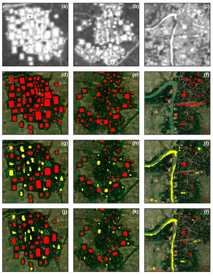
Figure 6.
Fishpond classification results of three example subarea. Red polygons represent fishponds and yellow polygons represent water bodies identified by spectral filtering and rejected by spatial filtering. From top to bottom row: Automated Water Extraction Index (AWEI) image on 30 April 2020 (a–c), ground truth data (d–f), classification results by DT (g–i), classification results by LR (j–l). Green circles in subfigure (g–l) highlight differences between results obtained from DT and LR.
Figure 7 shows another village with a few irregular-shaped fishponds, e.g., the ‘L’ shaped fishpond on the left side of the region labeled as 1. Both LR and DT misclassified most of the fishponds in this region. Specifically, fishpond 1 was misclassified because of its concave shape. As discussed in the methodology, OBFs are mostly designed to measure shape compactness and convexity, and the primary assumption of using OBFs to classify fishponds is that fishponds have relatively simpler shapes than other water objects. Fishpond 2 is in fact a group of small fishponds according to the ground truth data shown in Figure 7b. The overly small gaps between such small fishponds cannot be identified; thus, they were recognized as one giant fishpond with complex shapes. Lastly, fishpond 3 was misclassified due to its elongated shape. As a result, any small fluctuations on the longer side can significantly affect convex hull based OBFs, such as SOLI and CONV. The misclassification of fishpond 2 and 3 indicate the huge influence of spatial resolution on the fishpond recognition. Fishponds are generally small, and some of them are as small as 200 sq. meters, which is roughly 2 pixels on a Sentinel-2 image. The relatively coarse spatial resolution not only over-simplified boundaries of small fishponds but also amplifies the differences of OBFs caused by tiny changes to the shapes.
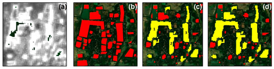
Figure 7.
Examples of unsatisfactory classification results. Red polygons represent fishponds and yellow polygons represent water bodies identified by spectral filtering and rejected by spatial filtering. From subfigure (a–d): AWEI image on 30 April 2020, ground truth data, classification results by DT, classification results by LR.
4.2. Validation Results
The proposed method was evaluated using the holdout testing dataset in 4 of the unions within the study area. The results are shown in Table 1. Specifically, the LR model identified in a total of 841 fishponds within the test unions, and the DT model identified 789 fishponds. Of all the classified fishponds, LR correctly classified 663 of the 841, and the precision score is 0.788. DT correctly classified 610 of 789, and the precision score is 0.773. As a comparison, the ground truth data contains in total 1232 fishponds within the test region. From Table 6, we can see that LR has dominantly better performance on the test dataset with all metric scores higher than DT even though DT performed better during training. The precision score of LR is 1.5% higher than DT, and the recall rate of LR is over 4% higher than DT. The overall F1 score of LR is 3.6% higher than DT. Therefore, LR is recommended to be implemented as the classifier for fishponds.
Table 6.
Evaluation of LR and DT on the test dataset.
5. Discussions
5.1. Importance of the Pixel Selection Technique
Figure 8 shows the comparison of histograms of WI values with and without pixel selection, as well as optimal thresholds derived by the Otsu method. From Figure 8, we can see that most of the histograms show bimodal distributions. One peak on the high-value side indicates water types, and the peak on the lower WI value side indicates other land cover types. Comparing thresholds derived using the Otsu method with and without pixel selection step, we can find that most threshold values are close such that whether to use pixel selection may not result in much difference. However, there are a few exceptions where the thresholds derived with pixel selection are quite different from that without. Specifically, thresholds derived with pixel selection on the NDWI image on January 1st and MNDWI and AWEI images on 30 April 2020 all fall out the valleys of the histograms, which significantly changes the class distributions of the segmented images. Figure 9 shows an example of such differences for the MNDWI image on 30 April 2020. Figure 9 clearly shows that the segmentation result with pixel selection is much better than without because the latter includes a lot of false positives, especially in the southwest region of the study area. Moreover, the boundaries of fishponds cannot be clearly identified due to the false positives, as shown in the upper right subfigures. The pixel selection is especially effective when the target class is scarce so that the difference between the target class and other classes is shadowed by variations within other classes. For example, the histograms of NDWI on 1 January 2020 and MNDWI on 30 April 2020 in Figure 8 show two peaks, and the Otsu method finds the threshold in the valley if no pixel selection is applied. However, such peaks just represent the internal variations of non-water types instead of between water class and non-water class. By applying the pixel selection technique, the number of non-water type pixels is significantly reduced to the same level as water features and thus produce better segmentation results. The thresholds derived using the Otsu method are shown in Table 7.
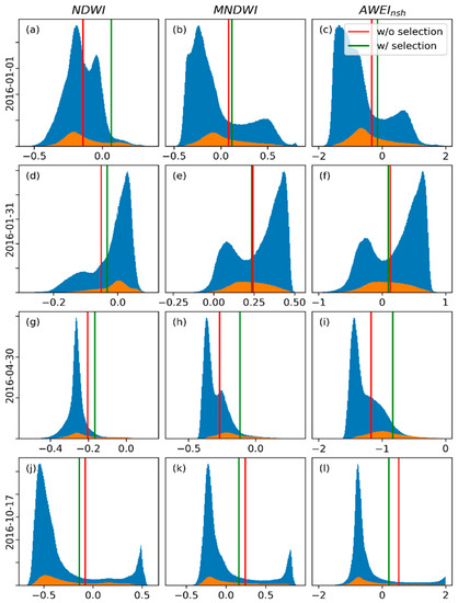
Figure 8.
Histograms of WIs for four image dates within the study area. Blue histograms: without pixel selection technique; orange histograms: with pixel selection technique. Each row, i.e., subfigure (a–c), (d–f), (g–i), and (j–l), contains histograms of NDWI, MNDWI, and AWEI for the study area at the corresponding image date.
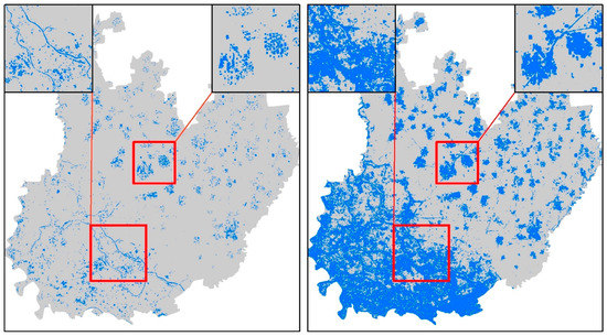
Figure 9.
Comparison of water feature segmentation results for the MNDWI image on April 30th. Left side: with pixel selection technique; right side: without pixel selection technique.
Table 7.
Otsu method derived thresholds for WIs. Left column: with pixel selection; right column: without pixel selection. Thresholds that lead to major difference are highlighted.
Figure 9 demonstrated the effectiveness of the pixel selection technique in mapping small water features with Sentinel-2 images. Similar approaches also proved their effectiveness when applied to commercial high-resolution satellite images [31] and medium resolution images, such as Landsat images [29]. This also indicates that the pixel selection technique, in general, can help map water features at continental and global scale in an unsupervised way because water features consist of only a small portion of the continents [36]. For supervised water feature classification, the pixel selection method can also help automatically generate training samples such that positive class samples and negative class samples are well balanced [45]. Lastly, the pixel selection technique can also help with water feature mappings with non-optical sensors, such as Synthetic Aperture Radar (SAR) [48] and Soil Moisture Active Passive (SMAP) [49,50], because microwave-based water feature mapping also depends on finding optimal thresholds.
5.2. Object-Based Features Comparisons
Five OBFs, i.e., IPQ, SOLI, PFD, CONV, and SqP were calculated for all vectorized all-year-inundated water features. Figure 10 shows the paired scatter plot of OBF values of training data samples. Specifically, the diagonal subfigures show the distribution of each OBF values for fishponds and non-fishpond types, and the off-diagonal subfigures show the scattered points on the 2D space of the corresponding OBF features. From the diagonal subfigures, we can see that IPQ, CONV, and SqP provide good class separability because the peaks of distributions are well separated, while the distributions of SOLI and PFD have a lot of overlap. From the most upper-right subplot, we can also see that SqP and IPQ show a near quadratic relationship as all points align on a simple curve. This can be proved using the formula of the two features. From all subfigures, the most likely feature pairs that may provide linear separability is the pair of PFD and SqP because the positive samples and negative samples roughly align along the opposite sides of the line visually. Other pairs of features do not show clear separability between the two classes.
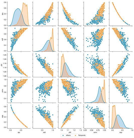
Figure 10.
Paired scatter plots of OBFs. Diagonal plots are histograms of each OBF for fishpond and non-fishpond classes. Off-diagonal plots are scatter plots of corresponding feature pairs of fishponds and non-fishponds samples.
5.3. Limitations and Future Work
The major limitation of the work is that the spatial resolution of Sentinel-2 images is not high enough to map extremely small-scale fishponds, which is common for house-owned inland fishponds in Bangladesh. A great portion of the inland fishponds are only a few pixels large such that the pixel outlines cannot accurately represent true shapes of these fishponds. As for now, Sentinel-2 is the only operational optical satellite that provides continuous and high-resolution multi-spectral data free of charge. Thus, until new missions are launched, Sentinel-2 10 m spatial resolution is the best for long-term and continuous mapping of inland fishponds. One promising direction to address the limitations caused by spatial resolution is sub-pixel mapping which produces LULC maps at the resolution higher than the input images [51,52,53,54]. Many research works have shown the great potential of improving mapping accuracies, especially when spatial resolution is too coarse to accurately show object boundaries. However, the effectiveness of sub-pixel mapping when applied to extremely small objects that are only a few pixels large is yet to be investigated.
Another limitation is that cloud covers in monsoon seasons limited the number of images that can be used. Thus, a few previous research works use SAR images instead of optical images for aquaculture pond mapping in South Asia [6,7]. As SAR uses microwave spectrum that can penetrate clouds, and it does not rely on the presence of sun, it can provide significantly better temporal coverage for regions with heavy cloud contaminations. Moreover, water features have very low backscatter when comparing with other LULC types such that they stand out on SAR images [40,48,55]. However, SAR images are generally contaminated with speckle noises that needs to be preprocessed by filtering, which will somewhat reduce the spatial resolution of the product, and edges may not be preserved. The reduced spatial resolution may not affect large objects mapping, such as coastal aquaculture ponds, it may have a major impact on the performance of mapping small-scale inland fishponds [55]. Recent research showed that the integrative usage of optical and SAR sensors, especially Sentinel-1 and Sentinel-2, has great potential in LULC mapping in monsoon area [56], and this is a very promising direction for improving the current state of inland fishpond mapping.
6. Conclusions
Inland fishery is growing fast in Bangladesh and many other South Asia countries, such as India. The underlying LULC change, especially the transition of agriculture land to aquaculture land may put pressure on already limited agriculture land for large populations. Mapping and monitoring inland fishponds are essential to understand such LULC changes. While there are many research works focused on mapping coastal aquaculture ponds, which share some similarities with inland fishponds, there is rarely any research focus on mapping inland fishponds that are typically small and unorganized. Thus, this research presented a workflow that uses multi-temporal Sentinel-2 images for fishpond mapping in the context of a case study in the Singra Upazila in Bangladesh. The workflow first applies a spectral-based filtering that automatically segments multi-temporal images using WIs and generates an all-year-inundated water feature mask. A key step in the spectral filtering is to apply a pixel selection technique that limit number of pixels used in image segmentation, which is essential to map small objects in a large area. Then, a spatial-based filtering was applied to classify all-year-inundated water objects into fishponds and non-fishponds using OBFs. We used five OBFs to characterize water objects and trained a LR and a DT model using the five OBFs as features. The LR model achieved better results than DT, and the trained LR model was used in the workflow for final classification. In a case study in the Singra Upazila in Bangladesh, we manually digitized fishponds using Google Earth historical images and tested our method. The proposed workflow achieved around 79% precision and 54% recall rate. Lastly, the workflow was implemented on GEE and thus can be easily reapplied to new regions.
Author Contributions
Conceptualization, Z.Y., L.D., and J.T.; methodology, Z.Y.; software, Z.Y.; validation, Z.Y. and M.S.R.; investigation, Z.Y., L.D., and M.S.R.; data curation, Z.Y. and M.S.R.; writing—original draft preparation, Z.Y.; writing—review and editing, Z.Y., L.D., M.S.R., and J.T.; supervision, L.D.; funding acquisition, L.D. and J.T. All authors have read and agree to the published version of the manuscript.
Funding
This study was supported by a grant from the National Aeronautics and Space Administration (NASA) Land Use and Land Cover Program (Award No. NNX17AH95G, PI: Liping Di).
Conflicts of Interest
The authors declare no conflict of interest.
References
- Hashem, S.; Akter, T.; Salam, M.A.; Tawheed Hasan, M.; Hasan, M.T. Aquaculture planning through Remote Sensing Image analysis and GIS tools in North east region, Bangladesh. Int. J. Fish. Aquat. Stud. IJFAS 2014, 1, 127–136. [Google Scholar]
- Shahin, J.; Fatema, M.K.; Fatema, J.; Mondal, M.N.; Rahman, M.M. Potentialities of pond fish farming in Kaliakair upazila under Gazipur district, Bangladesh. Res. Agric. Livest. Fish. 2015, 2, 517–528. [Google Scholar] [CrossRef]
- Thilsted, S.H. The potential of nutrient-rich small fish species in aquaculture to improve human nutrition and health. Farming Waters People Food Proc. Glob. Conf. Aquac. 2010, 2012, 57–73. [Google Scholar]
- Yu, Z.; Di, L.; Tang, J.; Zhang, C.; Lin, L.; Yu, E.G.; Rahman, M.S.; Gaigalas, J.; Sun, Z. Land Use and Land Cover Classification for Bangladesh 2005 on Google Earth Engine. In Proceedings of the 2018 7th International Conference on Agro-Geoinformatics (Agro-Geoinformatics) IEEE, Hangzhou, China, 6–9 August 2018; pp. 1–5. [Google Scholar]
- Gorelick, N.; Hancher, M.; Dixon, M.; Ilyushchenko, S.; Thau, D.; Moore, R. Google Earth Engine: Planetary-scale geospatial analysis for everyone. Remote Sens. Environ. 2017, 202, 18–27. [Google Scholar] [CrossRef]
- Ottinger, M.; Clauss, K.; Kuenzer, C. Large-Scale Assessment of Coastal Aquaculture Ponds with Sentinel-1 Time Series Data. Remote Sens. 2017, 9, 440. [Google Scholar] [CrossRef]
- Prasad, K.; Ottinger, M.; Wei, C.; Leinenkugel, P. Assessment of Coastal Aquaculture for India from Sentinel-1 SAR Time Series. Remote Sens. 2019, 11, 357. [Google Scholar] [CrossRef]
- Virdis, S.G.P. An object-based image analysis approach for aquaculture ponds precise mapping and monitoring: A case study of Tam Giang-Cau Hai Lagoon, Vietnam. Environ. Monit. Assess. 2014, 186, 117–133. [Google Scholar] [CrossRef]
- Belton, B.; Azad, A. The characteristics and status of pond aquaculture in Bangladesh. Aquaculture 2012, 358–359, 196–204. [Google Scholar] [CrossRef]
- Du, Y.; Zhang, Y.; Ling, F.; Wang, Q.; Li, W.; Li, X. Water bodies’ mapping from Sentinel-2 imagery with Modified Normalized Difference Water Index at 10-m spatial resolution produced by sharpening the swir band. Remote Sens. 2016, 8, 354. [Google Scholar] [CrossRef]
- Yang, X.; Qin, Q.; Grussenmeyer, P.; Koehl, M. Urban surface water body detection with suppressed built-up noise based on water indices from Sentinel-2 MSI imagery. Remote Sens. Environ. 2018, 219, 259–270. [Google Scholar] [CrossRef]
- Ludwig, C.; Walli, A.; Schleicher, C.; Weichselbaum, J.; Riffler, M. A highly automated algorithm for wetland detection using multi-temporal optical satellite data. Remote Sens. Environ. 2019, 224, 333–351. [Google Scholar] [CrossRef]
- McFeeters, S.K. The use of the Normalized Difference Water Index (NDWI) in the delineation of open water features. Int. J. Remote Sens. 1996, 17, 1425–1432. [Google Scholar] [CrossRef]
- Xu, H. Modification of normalised difference water index (NDWI) to enhance open water features in remotely sensed imagery. Int. J. Remote Sens. 2006, 27, 3025–3033. [Google Scholar] [CrossRef]
- Feyisa, G.L.; Meilby, H.; Fensholt, R.; Proud, S.R. Automated Water Extraction Index: A new technique for surface water mapping using Landsat imagery. Remote Sens. Environ. 2014, 140, 23–35. [Google Scholar] [CrossRef]
- Ji, L.; Zhang, L.; Wylie, B. Analysis of dynamic thresholds for the normalized difference water index. Photogramm. Eng. Remote Sens. 2009, 75, 1307–1317. [Google Scholar] [CrossRef]
- Zhou, Y.; Dong, J.; Xiao, X.; Xiao, T.; Yang, Z.; Zhao, G.; Zou, Z.; Qin, Y. Open surface water mapping algorithms: A comparison of water-related spectral indices and sensors. Water Switz. 2017, 9, 256. [Google Scholar] [CrossRef]
- Jiang, H.; Feng, M.; Zhu, Y.; Lu, N.; Huang, J.; Xiao, T. An automated method for extracting rivers and lakes from Landsat imagery. Remote Sens. 2014, 6, 5067–5089. [Google Scholar] [CrossRef]
- Huang, C.; Chen, Y.; Zhang, S.; Wu, J. Detecting, Extracting, and Monitoring Surface Water From Space Using Optical Sensors: A Review. Rev. Geophys. 2018, 56, 333–360. [Google Scholar] [CrossRef]
- Wang, Z.; Liu, J.; Li, J.; Zhang, D.D. Multi-SpectralWater Index (MuWI): A Native 10-m Multi-Spectral Water Index for Accurate Water mapping on sentinel-2. Remote Sens. 2018, 10, 1643. [Google Scholar] [CrossRef]
- Yu, Q.; Gong, P.; Clinton, N.; Biging, G.; Kelly, M.; Schirokauer, D. Object-Based detailed vegetation classification with airborne high spatial resolution remote sensing imagery. Photogramm. Eng. Remote Sens. 2006, 72, 799–811. [Google Scholar] [CrossRef]
- Jiao, L.; Liu, Y.; Li, H. Characterizing land-use classes in remote sensing imagery by shape metrics. ISPRS J. Photogramm. Remote Sens. 2012, 72, 46–55. [Google Scholar] [CrossRef]
- van der Werff, H.M.A.; van der Meer, F.D. Shape-Based classification of spectrally identical objects. ISPRS J. Photogramm. Remote Sens. 2008, 63, 251–258. [Google Scholar] [CrossRef]
- Song, C.; Huang, B.; Ke, L. Modeling and analysis of lake water storage changes on the Tibetan Plateau using multi-mission satellite data. Remote Sens. Environ. 2013, 135, 25–35. [Google Scholar] [CrossRef]
- Zhang, G.; Zheng, G.; Gao, Y.; Xiang, Y.; Lei, Y.; Li, J. Automated water classification in the Tibetan plateau using Chinese GF-1 WFV data. Photogramm. Eng. Remote Sens. 2017, 83, 509–519. [Google Scholar] [CrossRef]
- Razu Ahmed, M.; Rahaman, K.R.; Kok, A.; Hassan, Q.K. Remote sensing-based quantification of the impact of flash flooding on the rice production: A case study over Northeastern Bangladesh. Sens. Switz. 2017, 17, 2347. [Google Scholar] [CrossRef]
- Xiao, X.; Boles, S.; Liu, J.; Zhuang, D.; Frolking, S.; Li, C.; Salas, W.; Moore, B. Mapping paddy rice agriculture in southern China using multi-temporal MODIS images. Remote Sens. Environ. 2005, 95, 480–492. [Google Scholar] [CrossRef]
- Liu, H.; Jezek, K.C. Automated extraction of coastline from satellite imagery by integrating canny edge detection and locally adaptive thresholding methods. Int. J. Remote Sens. 2004, 25, 937–958. [Google Scholar] [CrossRef]
- Zhang, F.; Li, J.; Zhang, B.; Shen, Q.; Ye, H.; Wang, S.; Lu, Z. A simple automated dynamic threshold extraction method for the classification of large water bodies from landsat-8 OLI water index images. Int. J. Remote Sens. 2018, 39, 3429–3451. [Google Scholar] [CrossRef]
- Donchyts, G.; Schellekens, J.; Winsemius, H.; Eisemann, E.; van de Giesen, N. A 30 m resolution surfacewater mask including estimation of positional and thematic differences using landsat 8, SRTM and OPenStreetMap: A case study in the Murray-Darling basin, Australia. Remote Sens. 2016, 8, 386. [Google Scholar] [CrossRef]
- Cooley, S.; Smith, L.; Stepan, L.; Mascaro, J. Tracking Dynamic Northern Surface Water Changes with High-Frequency Planet CubeSat Imagery. Remote Sens. 2017, 9, 1306. [Google Scholar] [CrossRef]
- Sheng, Y.; Song, C.; Wang, J.; Lyons, E.A.; Knox, B.R.; Cox, J.S.; Gao, F. Representative lake water extent mapping at continental scales using multi-temporal Landsat-8 imagery. Remote Sens. Environ. 2016, 185, 129–141. [Google Scholar] [CrossRef]
- Otsu, N. A Threshold Selection Method from Gray-Level Histograms. IEEE Trans. Syst. Man Cybern. 2008, 9, 62–66. [Google Scholar] [CrossRef]
- Jakovljević, G.; Govedarica, M.; Álvarez-Taboada, F. Waterbody mapping: A comparison of remotely sensed and GIS open data sources. Int. J. Remote Sens. 2019, 40, 2936–2964. [Google Scholar] [CrossRef]
- Calvario Sanchez, G.; Dalmau, O.; Alarcon, T.E.; Sierra, B.; Hernandez, C. Selection and fusion of spectral indices to improve water body discrimination. IEEE Access 2018, 6, 72952–72961. [Google Scholar] [CrossRef]
- Kordelas, G.A.; Manakos, I.; Aragonés, D.; Díaz-Delgado, R.; Bustamante, J. Fast and automatic data-driven thresholding for inundation mapping with Sentinel-2 data. Remote Sens. 2018, 10, 910. [Google Scholar] [CrossRef]
- Yin, D.; Cao, X.; Chen, X.; Shao, Y.; Chen, J. Comparison of automatic thresholding methods for snow-cover mapping using Landsat TM imagery. Int. J. Remote Sens. 2013, 34, 6529–6538. [Google Scholar] [CrossRef]
- Tang, J.; Di, L.; Rahman, M.S.; Yu, Z. Spatial–Temporal landscape pattern change under rapid urbanization. J. Appl. Remote Sens. 2019, 13, 1. [Google Scholar] [CrossRef]
- Chen, R.; Li, X.; Li, J. Object-Based features for house detection from RGB high-resolution images. Remote Sens. 2018, 10, 451. [Google Scholar] [CrossRef]
- Liu, K.; Ai, B.; Wang, S. Fish-pond change detection based on short term time series of RADARSAT images and object-oriented method. In Proceedings of the 3rd International Congress on Image and Signal Processing, CISP, Yantai, China, 16–18 October 2010; Volume 5, pp. 2175–2179. [Google Scholar]
- Moser, D.; Zechmeister, H.G.; Plutzar, C.; Sauberer, N.; Wrbka, T.; Grabherr, G. Landscape patch shape complexity as an effective measure for plant species richness in rural landscapes. Landsc. Ecol. 2002, 17, 657–669. [Google Scholar] [CrossRef]
- Jitkajornwanich, K.; Vateekul, P.; Panboonyuen, T.; Lawawirojwong, S.; Srisonphan, S. Road map extraction from satellite imagery using connected component analysis and landscape metrics. In Proceedings of the 2017 IEEE International Conference on Big Data, Big Data, Boston, MA, USA, 11–14 December 2017; Volume 2018, pp. 3435–3442. [Google Scholar]
- Li, W.; Chen, T.; Wentz, E.A.; Fan, C. NMMI: A Mass Compactness Measure for Spatial Pattern Analysis of Areal Features. Ann. Assoc. Am. Geogr. 2014, 104, 1116–1133. [Google Scholar] [CrossRef]
- Frohn, R.C. The use of landscape pattern metrics in remote sensing image classification. Int. J. Remote Sens. 2006, 27, 2025–2032. [Google Scholar] [CrossRef]
- Pekel, J.-F.F.; Cottam, A.; Gorelick, N.; Belward, A.S. High-Resolution mapping of global surface water and its long-term changes. Nature 2016, 540, 418–422. [Google Scholar] [CrossRef] [PubMed]
- Breiman, L.; Friedman, J.; Stone, C.J.; Olshen, R.A. Classification and Regression Trees; CRC Press: Boca Raton, FL, USA, 1984. [Google Scholar]
- Kleinbaum, D.G.; Klein, M. Statistics for Biology and Health. In Logistic Regression; Springer: New York, NY, USA, 2010; ISBN 978-1-4419-1741-6. [Google Scholar]
- Zhou, S.; Kan, P.; Silbernagel, J.; Jin, J. Application of Image Segmentation in Surface Water Extraction of Freshwater Lakes using Radar Data. ISPRS Int. J. Geo-Inf. 2020, 9, 424. [Google Scholar] [CrossRef]
- Du, J.; Kimball, J.S.; Galantowicz, J.; Kim, S.-B.; Chan, S.K.; Reichle, R.; Jones, L.A.; Watts, J.D. Assessing global surface water inundation dynamics using combined satellite information from SMAP, AMSR2 and Landsat. Remote Sens. Environ. 2018, 213, 1–17. [Google Scholar] [CrossRef]
- Rahman, M.; Di, L.; Yu, E.; Lin, L.; Zhang, C.; Tang, J. Rapid Flood Progress Monitoring in Cropland with NASA SMAP. Remote Sens. 2019, 11, 191. [Google Scholar] [CrossRef]
- Foody, G.M.; Muslim, A.M.; Atkinson, P.M. Super-Resolution mapping of the waterline from remotely sensed data. Int. J. Remote Sens. 2005, 26, 5381–5392. [Google Scholar] [CrossRef]
- Su, Y.-F. Integrating a scale-invariant feature of fractal geometry into the Hopfield neural network for super-resolution mapping. Int. J. Remote Sens. 2019, 1–22. [Google Scholar] [CrossRef]
- Li, L.; Chen, Y.; Yu, X.; Liu, R.; Huang, C. Sub-Pixel flood inundation mapping from multispectral remotely sensed images based on discrete particle swarm optimization. ISPRS J. Photogramm. Remote Sens. 2015, 101, 10–21. [Google Scholar] [CrossRef]
- Ling, F.; Zhang, Y.; Foody, G.M.; Li, X.; Zhang, X.; Fang, S.; Li, W.; Du, Y. Learning-Based Superresolution Land Cover Mapping. IEEE Trans. Geosci. Remote Sens. 2016, 54, 3794–3810. [Google Scholar] [CrossRef]
- Shen, X.; Wang, D.; Mao, K.; Anagnostou, E.; Hong, Y. Inundation Extent Mapping by Synthetic Aperture Radar: A Review. Remote Sens. 2019, 11, 879. [Google Scholar] [CrossRef]
- Steinhausen, M.J.; Wagner, P.D.; Narasimhan, B.; Waske, B. Combining Sentinel-1 and Sentinel-2 data for improved land use and land cover mapping of monsoon regions. Int. J. Appl. Earth Obs. Geoinf. 2018, 73, 595–604. [Google Scholar] [CrossRef]
© 2020 by the authors. Licensee MDPI, Basel, Switzerland. This article is an open access article distributed under the terms and conditions of the Creative Commons Attribution (CC BY) license (http://creativecommons.org/licenses/by/4.0/).