1. Introduction
Ground-penetrating radar (GPR) has long been used for determining the location, depth, and shape of human burials e.g., [
1,
2,
3,
4,
5,
6]. Because of its non-invasive approach, rapid data acquisition, and real-time data viewing, GPR is an ideal method for forensic and archaeological applications. Nevertheless, the method does suffer from several significant limitations, including, but not limited to, high electromagnetic signal attenuation (loss of signal with depth), scattering (energy reflected in multiple directions), and false positives (misidentification) from roots or other buried objects (e.g., [
3,
7,
8]). Although GPR has been well studied and applied across many disciplines, extracting sharp images (highlighting desired anomalies while minimizing unwanted features) through signal processing remains a challenge.
The GPR response of a grave is sometimes a diffraction pattern (hyperbola-shaped signature often produced by point-like targets) or a disturbed section of strata. In both scenarios, interpretations can be limited. For example, migration algorithms collapse diffraction events to single points that are positioned at a depth corresponding to the diffraction apex to produce a more realistic representation of the subsurface [
9]. However, other nearby buried features (i.e., cobbles, tree roots, or ringing from shallower features) are erroneously incorporated into the migration scheme. The result is anomalies that comprise more than one target, making it challenging to distinguish individual buried objects.
Singular value decomposition (SVD) is an advantageous filtering technique: reduce high-dimensional, highly variable data to a lower-dimensional space that reveals substructures, discard the unwanted substructures (i.e., direct wave, ringing, random noise), and reconstruct a filtered image. SVD has been previously applied to GPR data e.g., [
10,
11,
12,
13,
14,
15,
16,
17] with much success. In particular, SVD has been used to increase the resolution of small, point-like reflections in GPR [
11]. The whole approach is computationally efficient and ideal for data sets in which the targets and non-targets have non-horizontal geometries [
10] and contrasting amplitudes [
17].
In areas with variable relief, a topographic correction of GPR data should be performed either as a topographic migration [
18,
19] or simply a static shift [
20]. In areas of very low but observable relief, a static shift following migration is sufficient. Global Positioning Systems (GPS) can be paired with GPR equipment to synchronously collect geospatial and geophysical data. It has been shown that high-precision height information is valuable in archaeological settings e.g., [
21,
22,
23,
24,
25]. Digital elevation models (DEM) derived from airborne laser scanning (ALS) datasets can provide full coverage of a survey area (ALS is also referred to as airborne Light Detection and Ranging or airborne LiDAR). Elevation can also be extracted from point cloud data e.g., [
24,
25,
26,
27] to perform a topographic correction of GPR data. Alternatively, elevation models derived from terrestrial laser scan (TLS) data provide a higher horizontal and vertical resolution that can reveal subtle mounds or depressions that may correspond to subsurface features [
28].
This paper presents the geophysical findings from the Wilson Brothers Cemetery on Cape Canaveral Air Force Station, Florida (CCAFS,
Figure 1a) and the joint data processing and remote sensing techniques used to increase GPR image resolution and refine the shape and depth of anomalies. We show that SVD can remove ringing that overprints targets of interest and improves migration results. We then perform topographic corrections while using elevation derived from TLS and ALS to highlight subtle topographic changes that can influence GPR data interpretation. The techniques themselves are well-known, but have not been jointly applied to detect and characterize burials.
1.1. Historical Context
Many Anglo-American homesteaders moved to Cape Canaveral after the Civil War to exploit expanded economic ventures in the fishing and agricultural industries. Eight cemeteries were established on the cape dating from the late 1800s to mid-1950s, mostly small family plots, one community cemetery, and two believed to be single burials. The United States government began purchasing land on the island in the late 1930s in order to establish a long-range proving ground for missiles. By 1952, the entirety of the cape was federal land. As a cape occupied for at least 3000 years [
29,
30], the remains of several distinct archaeological site types, including the eight historic cemeteries, are spatially intertwined with the iconic launch complexes and Air Force facilities that are embedded with historical significance.
Most of the cemeteries were left abandoned or poorly maintained until relatively recently. The chain-link fences that border each cemetery are not original and are considered arbitrary boundaries. The exact footprint of each cemetery is unknown, and many cemeteries were speculated to have unmarked burials. Therefore, in support of CCASF cultural resource management GPR, GPS, and TLS were undertaken at each cemetery in order to verify cemetery extent and locate any evidence of unmarked burials.
The Wilson Brothers Cemetery, recorded with the Florida Master Site File as 8BR3366, is a small Christian family plot that includes two known graves, Frank and Alfred Wilson. They are grandchildren of the locally well-known Mills Burnham, the first permanent lighthouse keeper on Cape Canaveral. Frank and Alfred were both born on the island and passed away in 1940 and 1942, respectively. Any specific religious denomination that would influence burial practices is unknown.
The fenced area is approximately 126 square meters. Within the fence, two east-facing headstones are enclosed by railroad ties that are approximately 15 cm × 15 cm × 2 m planks of wood (
Figure 1b). Shell midden material, attributable to an ancient archaeological site, is also present in this area, but appears scattered and ephemeral.
The railroad ties present a challenge not encountered at the other cemeteries. The GPR signal from the ties is high amplitude ringing—coherent noise where a reverberating response from an object oscillates far longer than the GPR pulse. That oscillation is recorded as repeating reflections when, in reality, it is the energy reflected off of a single object. This site required the use of filtering techniques that the remaining cemetery datasets did not.
1.2. Physical Context
The surficial geology of CCAFS comprises unconsolidated deposits of fine- to medium-grain sand, silt, shell, and clay over limestone [
31,
32,
33]. The cemetery is located on the west coast of the cape along a north-south trending sand ridge. The environment is generally characterized by high infiltration rates [
34]. Soil cores taken in the vicinity of the cemetery show varying ratios of shell, sand, and silt down to at least 7 m [
35]. Beneath these sediments, clay content increases with depth. Bulk soil composition is an important consideration, because shells can produce numerous high amplitude reflections, and radar does not penetrate clay. The depth of investigation for this study does not intersect with clay layers. High shell content (natural and cultural) in the uppermost material is considered in data interpretations.
2. Materials and Methods
Common-offset (fixed distance between the transmitter and receiver) GPR data were collected with a 500 MHz shielded antenna and MALÅProEx system, where the system was mounted on a cart and pushed along the ground surface. Transects were collected in a grid and spaced 0.5 m apart and oriented perpendicular to presumed burial orientation. The trace interval (distance between scans) for all transects is 0.025 m. The cart odometer recorded transect distance. This level of spatial sampling does not obtain full resolution of the subsurface [
36], but enough to resolve burial-sized targets and disturbed strata. Geophysical data are protected according to 2019 Florida Statutes Title XVIII, Chapter 267.
GPS information was collected from all surface features (i.e., trees, tree stumps, fence corners, grave markers) and the start and stop position of each GPR transect—defined as the center position of the antenna. Field collection was performed using a Trimble GeoExplorer GeoXH Network Rover with a Zephyr2 antenna compatible with the sub-meter and centimeter package post-processing.
A simple dewow and time-zero correction were performed on each profile before SVD to remove inherent low-frequency noise and designate the starting point of the received signal, respectively. Singular value decomposition was performed in MATLAB (see
Appendix A for details); the code is available in
Supplementary. Reconstructed GPR data were transferred to GPR-SLICE for positioning, migration, three-dimensional (3D) volume interpolation, and topographic correction. We used hyperbola-fitting to estimate a single velocity of 0.16 m/ns, which reflect the dry conditions during data acquisition.
The 3D volumes were obtained in GPR-SLICE by sampling all profiles over the same increments of two-way travel time (2.9 ns) to produce 40 binned slices. The amplitudes of each bin are the average of values sampled within that bin. The slices were gridded at a 0.05 m cell size with inverse distance interpolation between samples of a given slice. The 3D volume is comprised of these grids and interpolations between them. Surface elevations that were derived from ALS and TLS were each imported for separate topographic corrections. Each dataset was gridded over the same cell size as the GPR data (0.05 by 0.05 m). The 3D volume was then draped over topography. Topographic profiles were also extracted to perform a static shift on select GPR profiles.
ALS data were published in 2007 by the Florida Division of Emergency Management [
37]. These have 1 m horizontal accuracy and 0.18 m vertical accuracy. Only points classified as ground were included in producing the 30-cm DEM. The DEM is available in
Supplementary.
A hybrid phase-shift scanner (Leica RTC360) was used in the TLS survey. Eight scans were collected in the fall of 2019. Data capture included all surface locations within the cemetery boundary. The scans were registered using native to scanner Cyclone software. The registration error was less than 5 mm on average. The final point cloud has a minimum point spacing of 5 mm along the ground.
A digital elevation model (DEM) was produced by georeferencing the TLS point cloud. The global horizontal positions of cemetery fence corner posts provide four reference points that were aligned with corresponding points in the TLS point cloud while using the open-source software CloudCompare. The corner elevations were extracted from the ALS-derived DEM. The wider scale terrain trends between ALS and TLS agree, so reference point elevations serve as elevation controls for otherwise arbitrary TLS height values. The main objective was to resolve small terrain differences within the cemetery. Once the TLS point cloud was georeferenced, all surface features (trees, fencing, headstones) were removed.
Both elevation datasets were gridded with 0.05 m cell size with inverse distance interpolation, which is the same cell size of the GPR depth slices. Because the ground is maintained grass, a minimum elevation value was assigned to each cell for the TLS data. The ALS-derived DEM has 30 cm resolution so the smaller cell size gained no resolution. TLS point clouds have subcentimeter scale resolution. Thus, the resolution was decreased by gridding to that of the GPR depth slices. Nevertheless, the detail captured by TLS and not ALS is still apparent.
3. Results
A total of 24 subparallel GPR transects (212.5 m) were collected over the Wilson Brothers Cemetery in a northeast-southwest direction. The closest soil core (approximately 1.5 km to the south) indicates 1.5 m of sand underlain by another 1.5 m of shell-rich sand. GPR data show the top of a semicontinuous layer of high amplitude reflectors at about 2.5 m depth, which is interpreted as the top of shell-rich sediments. Two anomalies that were identified as burials produce clear diffraction patterns in several successive profiles.
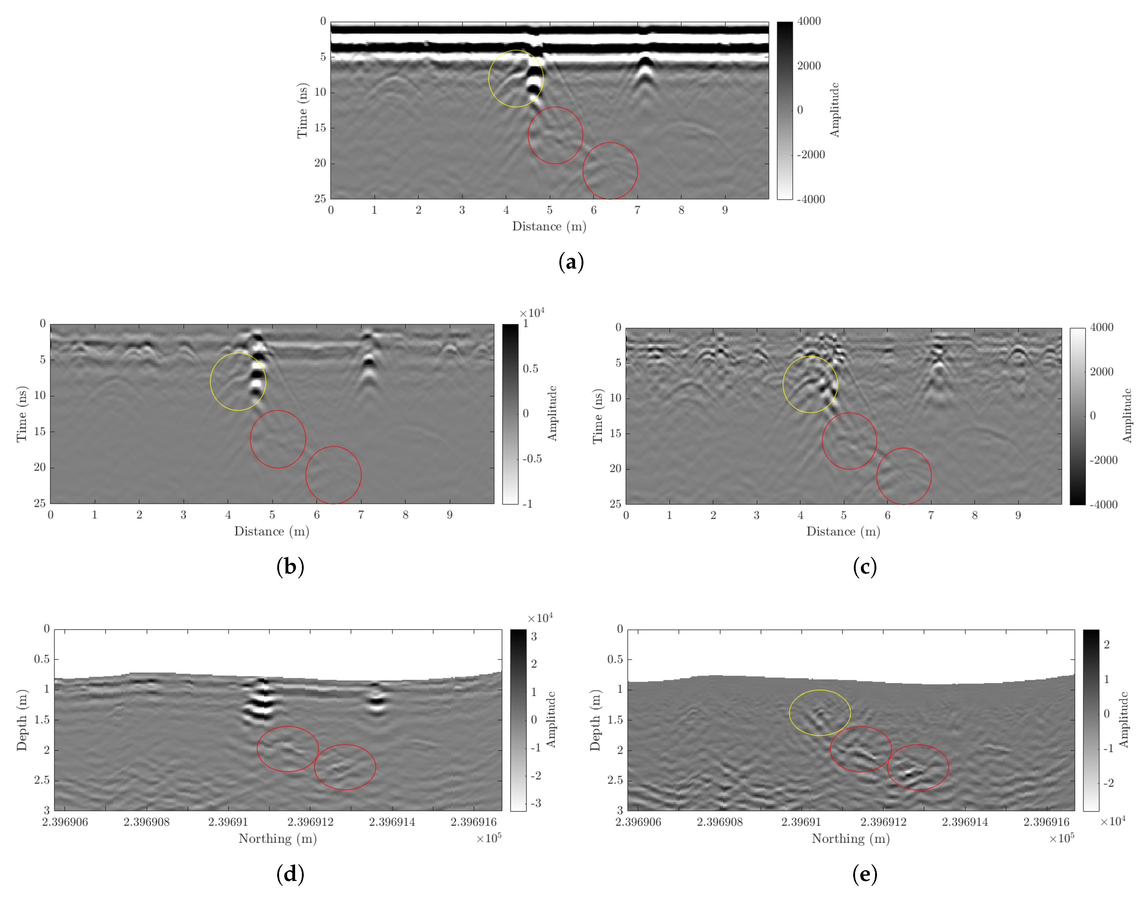
Figure 2 presents an example profile crossing over the burials.
The partially buried railroad ties produced very strong ringing down to about a meter depth (
Figure 2a, x = 4.5, 7 m). This ringing overprints a third diffraction pattern detected in several profiles. Although the diffraction is recognizable in profile view, it is difficult to resolve in depth slices due to the overprinting.
3.1. Singular Value Decomposition of GPR Data
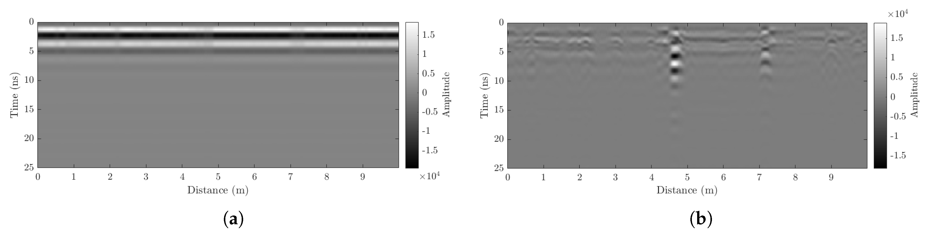
We must remove the direct wave (the received pulse traveling directly to the receiver) and the ringing to reveal the depth and extent of the overprinted diffractions. A standard mean trace subtraction (a.k.a background removal) successfully removes much of the direct wave; however, the ringing is entirely untouched (
Figure 2b). Rather than choosing a variety of trace widths through trial and error to calculate the best trace mean, we isolate the ringing and pull it out of the profile with SVD. A detailed explanation of the SVD approach is in
Appendix A.
SVD decomposes the GPR image into weighted eigenimages. To give the reader an idea of how much an image is decomposed, in the example profile in
Figure 2, SVD returned 390 eigenimages. As expected, the direct wave is the most dominant structure and captured in the first eigenimage (
Figure A1a). The ringing produced by the railroad ties at the surface is captured in the second through fifth eigenimages (
Figure A1b). A reconstructed GPR image—summing all but the first five eigenimages—now reveals reflections coming from the bottom of the railroad ties and the third diffraction that may or may not be associated with the burial plot (
Figure 2c). A large amount of energy is removed in the process, which is expected as the lowest eigenimage indices hold the most energy. Thus, an automatic gain control is applied after migration, but before creating a 3D volume and topographic correction.
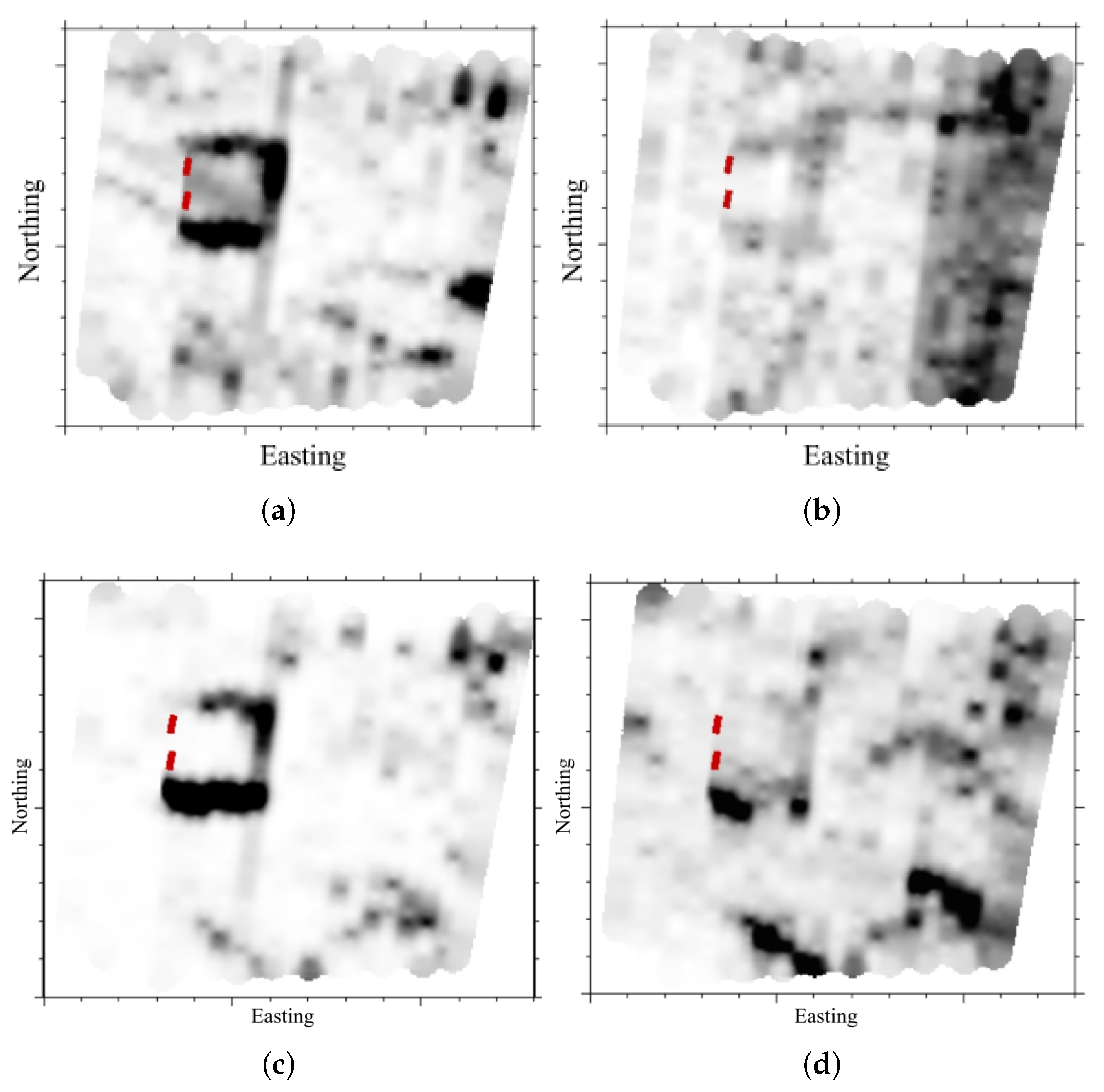
In map view, ringing that is produced by the railroad ties is most apparent at the surface where it is essentially the only feature detected. (
Figure 3a). SVD was performed, as described above, on all the GPR profiles before migration, gain, and topographic correction. The ringing is almost completely removed in map view (
Figure 3b). At a depth of 0.5 m, the ringing is still apparent overprinting a shallow anomaly. Furthermore, the ringing and anomaly combined appear as a relatively wider section of the railroad ties (
Figure 3c). With SVD performed on all profiles, the same shallow anomaly can be resolved as one or two features beneath the southern railroad tie (
Figure 3d). A tree root system in the eastern half of the grid is also more apparent.
3.2. Migration of SVD-Filtered GPR Data
We performed a two-dimensional (2D) Kirchhoff migration before and after SVD using a constant ground velocity (0.16 m/ns calculated from diffraction hyperbola fitting). It has been shown that TLS can be utilized to determine a best fit ground velocity [
24]. However, that is only possible when TLS data have captured subsurface structures (e.g., a cave or tunnel). We also acknowledge that a velocity profile would be more appropriate for resolving targets over a range of depths [
19]. The depth of investigation in this study is only the first two meters, and a single velocity fits the diffraction patterns within that range.
Migration that includes the ringing has multiple issues. First, the velocity of the ringing differs from the ground where target diffractions are. The chosen velocity may appropriately collapse diffractions (
Figure 2d, red circles), but it is an overestimate for the ringing. As a result, the signal of the ringing is spread out and obscures nearby features even more. Second, the ringing and diffraction pattern it overprints are collapsed together to an erroneously large single point reflector.
The migration of the SVD-filtered data produces more spatially constrained reflectors in the absence of ringing (
Figure 2e). One can see what is interpreted as the bottom of the railroad ties at about 0.5 m below the surface. Additionally, a third point-like anomaly (
Figure 2e, yellow circle) beneath the ties are observed where only two are discernible in the original data. The ability to migrate the two targets of interest at depth does not appear to be negatively affected by SVD.
3.3. Topographic Correction Using Elevations from ALS and TLS
Elevation comes from ALS- and TLS-derived elevation models (
Figure 4a,b, respectively). The ALS DEM measures a depression east of the graves that is not detected by TLS. Rather, TLS shows a square-shaped mound corresponding to the graves’ location, which is built-up gravel bounded by the railroad ties.
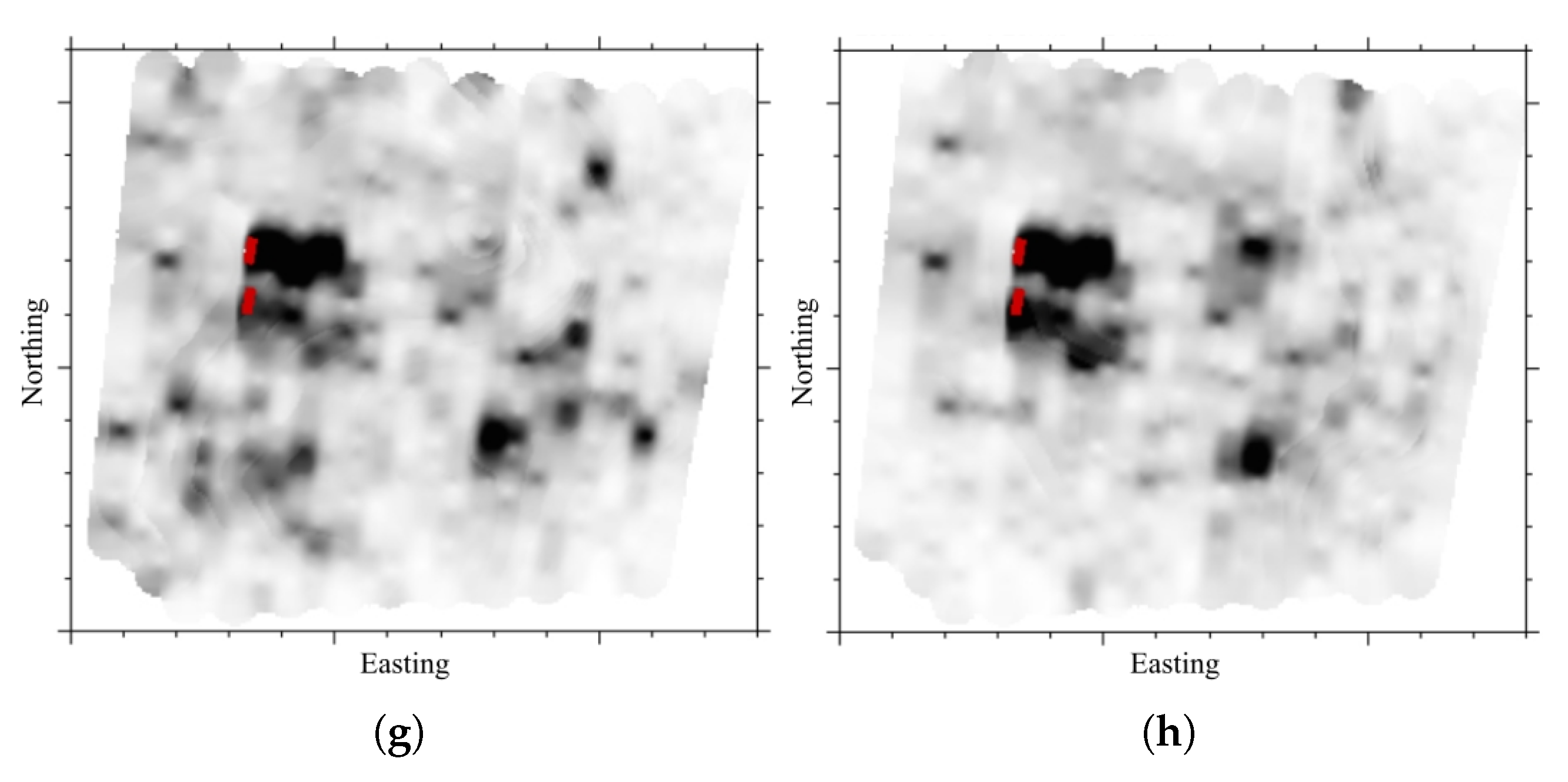
The variations between DEMs are small but enough to cause slightly different anomalies to appear in a given elevation slice. We illustrate this by presenting a pair of elevation slices for a target of interest where one dataset is topographically corrected with ALS-derived elevations and the other with TLS-derived elevations (
Figure 5). The targets are all approximately 20 cm higher in elevation when shifted by TLS values versus ALS values (
Figure 5e,f). The exception is the northernmost burial (
Figure 5g,h). This feature is 30 cm higher in TLS elevation slices, which is expected. This area corresponds to the edge of a depression in the ALS DEM, but not in the TLS DEM.
Beyond the targets of interest, there is disagreement between elevation slices. Tree roots extending into the survey area from the east and southeast appear to differing degrees between slices. Additionally, the northern burial appears to be at the same ALS elevation as the very top of the shell-rich sand layer. However, this layer does not appear level with the burial at TLS elevations.
4. Discussion
We encounter significant noise in a GPR dataset from a cemetery. Railroad ties that surround two graves produce ringing that overprints a anomaly of interest. SVD ranks structures in a GPR image in order of energy contribution. Because the ringing is such high amplitude and so spatially limited, it is captured in the first handful of eigenimages and, thus, easily omitted in data reconstruction.
SVD successfully removes the direct wave and the ringing to reveal overprinted diffractions. This improves the ability of the migration scheme (in this case, 2D Kirchhoff migration) to collapse single diffractions to point reflectors rather than incorporating signal from multiple features and producing erroneously large anomalies. Migrating the SVD-filtered GPR images yields more distinct and spatially constrained point reflectors. Furthermore, because signal ringing and diffractions produced by reflections are due to differing wave behavior, the ground velocity for a diffraction would only have made ringing more of a nuisance. Removing it allows for cleaner migration results.
SVD as a filtering technique is user-driven and data-dependent. One can rely on the first eigenimage to remove the direct wave, as other authors have shown. However, subsequent choices meant to remove unwanted signal will depend on (1) whether the amplitude of the reflected signal from a target of interest and “noise” are similar or (2) whether the unwanted signal exhibits the same geometry as the target signal. In archaeological settings, SVD may be successful in isolating targets such as graves and refuse pits from layered features, like shell midden or compacted ground. Again, one would need to produce the eigenimages and decide what can be filtered and what cannot.
At such a small scale (<150 square meter area), subtle relief can influence small geophysical targets’ depth and shape. We show that the marked burials are not associated with a depression, as measured by ALS. Instead, they are situated beneath a subtle modern mound bounded by the railroad ties as measured by TLS. ALS data, collected in 2007, have approximately 20 cm vertical accuracy. The horizontal accuracy is 1 m. We did not know of any physical changes that would have altered the site’s relief. We attribute the elevation differences to source data resolution.
The targets of interest are at approximately 20 cm higher elevation if we perform a topographic correction using TLS versus ALS. The difference is slightly larger (30 cm) for the northern confirmed burial. Under some circumstances, this is an insignificant variation. However, in archaeological applications, a notable change is often recorded at the sub-centimeter (certainly sub-meter) scale. Thus, the highest vertical resolution possible is preferred.
When presenting 3D GPR data as depth slices (no elevation applied), the elevation is inconsequential because the depth to a target is dependent on estimated ground velocities. Data interpretations from elevation slices, on the other hand, requires more careful attention in terms of the elevation source and resolution. In the example presented here, the confirmed burials have a similar vertical relationship, regardless of the elevation source. However, they are closer in depth, according to TLS versus ALS-derived elevations. Additionally, other features, like tree roots and the top of a shell-rich sand layer, are situated at different elevations. If these features were the intended target, the elevation source would influence in their depth and extent as well.
5. Conclusions
Geophysical interpretations are dependent on data quality and confidence in the location of anomalies relative to each other. This is especially true of GPR data from an archaeological setting where anomalies are small and shallow, and depth slices are preferred modes of presentation. Through the joint application of a subspace projection method and static topographic correction using surface elevation tomography, we show increased spatial resolution of two burials from a cemetery with two original headstones and a third feature that may or may not be associated with the burials. Terrain variations between the two elevation sources presented are small, but can be significant in the context of archaeological investigations.
Author Contributions
CRedit author statement: C.D.: Conceptualization, Data curation, Formal analysis, Investigation, Methodology, Software, Writing—Original draft preparation, Writing—Review and editing, Validation, Visualization; J.R.: Investigation, Writing—original draft preparation, Writing—review and editing; L.C.: Funding acquisition, Project administration, Resources, Supervision, Writing—Review and editing; T.D.: Funding acquisition, Resources. All authors have read and agreed to the published version of the manuscript.
Funding
The data used in this work was acquired for a project supported by Argonne National Laboratories [contract number 8F-30201] granted to Lori Collins and Travis Doering.
Acknowledgments
Thank you to Alexandra Kulenguski, Brett Parbus, Danielle Waite, and Danielle Young for their assistance collecting field data. Thank you to Jorge González García and Kyutae (Simon) Ahn for their assistance in preparing TLS data.
Conflicts of Interest
The authors declare no conflict of interest. The funders had no role in the design of this study; in the collection, analyses, or interpretation of data; in the writing of the manuscript, or in the decision to publish the results.
Abbreviations
The following abbreviations are used in this manuscript:
| ALS | Airborne laser scanning |
| CCAFS | Cape Canaveral Air Force Station |
| DEM | Digital elevation model |
| GPR | Ground-penetrating radar |
| GPS | Global positioning system |
| SVD | Singular value decomposition |
| TLS | Terrestrial laser scanning |
Appendix A. Singular Value Decomposition
Singular value decomposition (SVD) is a factorization of an
matrix
into orthogonal matrices in the form:
where
is the matrix of column eigenvectors of
and
is the matrix of row eigenvectors of
.
is a diagonal matrix of singular values of
is decreasing order.
A powerful feature of SVD is the ability to take high-dimensional, highly variable data, and reduce it to a lower-dimensional space that reveals substructures. We treat a GPR image as an m x n matrix where m is the number of traces, and n is the number of samples per trace. It can be written as:
where
r is the rank of
(the number of linearly independent traces),
is
ith singluar value of
,
is the
ith eigenvector of
, and
is the
ith eigenvector of
.
Eigenimages are linearly independent components of the GPR image. Singular values are the energy contribution factor of a given eigenimage. For example, the first (and largest) singular value corresponds to the eigenimage that contributes the most to the whole composition, which, in GPR, is he direct wave [
10,
15,
38].
Figure A1.
Substructures identified as unwanted signal and removed from the example GPR image shown in
Figure 2. (
a): The first eigenimage contains the most dominant substructures from a given GPR image—the direct wave. Horizontal banding is also a dominant structure in this example profile. (
b): The second through fifth eigenimages contain the ringing produced by the railroad ties. (
a) First Eigenimage from Example Profile. (
b) Second through Fifth Eigenimage from Example Profile.
References
- Nobes, D.C. The search for “Yvonne”: A case example of the delineation of a grave using near-surface geophysical methods. J. Forensic Sci. 2000, 45, 715–721. [Google Scholar] [CrossRef] [PubMed]
- Conyers, L.B. Ground-penetrating radar techniques to discover and map historic graves. Hist. Archaeol. 2006, 40, 64–73. [Google Scholar] [CrossRef]
- Jol, H.M. Ground Penetrating Radar Theory and Applications; Elsevier: Amsterdam, The Netherlands, 2008. [Google Scholar]
- Pringle, J.K.; Jervis, J.R.; Hansen, J.D.; Jones, G.M.; Cassidy, N.J.; Cassella, J.P. Geophysical Monitoring of Simulated Clandestine Graves Using Electrical and Ground-Penetrating Radar Methods: 0–3 Years After Burial. J. Forensic Sci. 2012, 57, 1467–1486. [Google Scholar] [CrossRef] [PubMed]
- Schultz, J.J. The application of ground-penetrating radar for forensic grave detection. In A Companion to Forensic Anthropology; Wiley: Hoboken, NJ, USA, 2012; pp. 85–100. [Google Scholar]
- Bradford, J.H. Ground-penetrating radar surveys of late-19th and early-20th century cemeteries to identify unmarked graves in rural Idaho, USA. In SEG Technical Program Expanded Abstracts 2018; Society of Exploration Geophysicists: Tulsa, OK, USA, 2018; pp. 2652–2656. [Google Scholar]
- Annan, A.P. GPR methods for hydrogeological studies. In Hydrogeophysics; Springer: Berlin/Heidelberg, Germany, 2005; pp. 185–213. [Google Scholar]
- Conyers, L.B. Analysis and interpretation of GPR datasets for integrated archaeological mapping. Near Surf. Geophys. 2015, 13, 645–651. [Google Scholar] [CrossRef]
- Yilmaz, Ö. Seismic Data Analysis: Processing, Inversion, and Interpretation of Seismic Data; Society of Exploration Geophysicists: Tulsa, OK, USA, 2001. [Google Scholar]
- Cagnoli, B.; Ulrych, T. Singular value decomposition and wavy reflections in ground-penetrating radar images of base surge deposits. J. Appl. Geophys. 2001, 48, 175–182. [Google Scholar] [CrossRef]
- Abujarad, F.; Jostingmeier, A.; Omar, A. Clutter removal for landmine using different signal processing techniques. In Proceedings of the Tenth International Conference on Grounds Penetrating Radar, Delft, The Netherlands, 21–24 June 2004; pp. 697–700. [Google Scholar]
- Kim, J.H.; Cho, S.J.; Yi, M.J. Removal of ringing noise in GPR data by signal processing. Geosci. J. 2007, 11, 75–81. [Google Scholar] [CrossRef]
- Nan, F.; Zhou, S.; Wang, Y.; Li, F.; Yang, W. Reconstruction of GPR signals by spectral analysis of the SVD components of the data matrix. IEEE Geosci. Remote Sens. Lett. 2009, 7, 200–204. [Google Scholar] [CrossRef]
- Zheng, J.; Peng, S.P.; Yang, F. A novel edge detection for buried target extraction after SVD-2D wavelet processing. J. Appl. Geophys. 2014, 106, 106–113. [Google Scholar] [CrossRef]
- Liu, C.; Song, C.; Lu, Q. Random noise de-noising and direct wave eliminating based on SVD method for ground penetrating radar signals. J. Appl. Geophys. 2017, 144, 125–133. [Google Scholar] [CrossRef]
- Bi, W.; Zhao, Y.; An, C.; Hu, S. Clutter elimination and random-noise denoising of GPR signals using an SVD method based on the Hankel matrix in the local frequency domain. Sensors 2018, 18, 3422. [Google Scholar] [CrossRef] [PubMed]
- Downs, C.; Jazayeri, S.; Collins, L.; Doering, T. Joint Application of High-pass Eigenimages and Sparse Blind Deconvolution for Improved Reflectivity Models of Historic Graves. In 18th International Conference on Ground Penetrating Radar Technical Program Expanded Abstracts; Society of Exploration Geophysicists: Tulsa, OK, USA, 2020. [Google Scholar]
- Lehmann, F.; Green, A.G. Topographic migration of georadar data: Implications for acquisition and processingTopographic Migration of Georadar Data. Geophysics 2000, 65, 836–848. [Google Scholar] [CrossRef]
- Allroggen, N.; Tronicke, J.; Delock, M.; Böniger, U. Topographic migration of gpr data with variable velocities. In Proceedings of the 2013 7th International Workshop on Advanced Ground Penetrating Radar, Nantes, France, 2–5 July 2013; pp. 1–5. [Google Scholar]
- Annan, A. Topographic Corrections of GPR Data; Technical Note; Sensors& Software Inc.: Mississauga, ON, Canada, 1991. [Google Scholar]
- Barratt, G.; Gaffney, V.; Goodchild, H.; Wilkes, S. Survey at Wroxeter using carrier phase, differential GPS surveying techniques. Archaeol. Prospect. 2000, 7, 133–143. [Google Scholar] [CrossRef]
- Kvamme, K.L.; Ernenwein, E.G.; Markussen, C.J. Robotic total station for microtopographic mapping: An example from the Northern Great Plains. Archaeol. Prospect. 2006, 13, 91–102. [Google Scholar] [CrossRef]
- Böeniger, U.; Tronicke, J. Improving the interpretability of 3D GPR data using target–specific attributes: Application to tomb detection. J. Archaeol. Sci. 2010, 37, 360–367. [Google Scholar] [CrossRef]
- Conejo-Martín, M.A.; Herrero-Tejedor, T.R.; Lapazaran, J.; Perez-Martin, E.; Otero, J.; Prieto, J.F.; Velasco, J. Characterization of cavities using the GPR, LIDAR and GNSS techniques. Pure Appl. Geophys. 2015, 172, 3123–3137. [Google Scholar] [CrossRef]
- Colucci, R.; Forte, E.; Boccali, C.; Dossi, M.; Lanza, L.; Pipan, M.; Guglielmin, M. Evaluation of internal structure, volume and mass of glacial bodies by integrated LiDAR and ground penetrating radar surveys: The case study of Canin Eastern Glacieret (Julian Alps, Italy). Surv. Geophys. 2015, 36, 231–252. [Google Scholar] [CrossRef]
- Colomina, I.; Molina, P. Unmanned aerial systems for photogrammetry and remote sensing: A review. ISPRS J. Photogramm. Remote Sens. 2014, 92, 79–97. [Google Scholar] [CrossRef]
- Puliti, S.; Ørka, H.O.; Gobakken, T.; Næsset, E. Inventory of small forest areas using an unmanned aerial system. Remote Sens. 2015, 7, 9632–9654. [Google Scholar] [CrossRef]
- Aziz, A.S.; Stewart, R.R.; Green, S.L.; Flores, J.B. Locating and characterizing burials using 3D ground-penetrating radar (GPR) and terrestrial laser scanning (TLS) at the historic Mueschke Cemetery, Houston, Texas. J. Archaeol. Sci. Rep. 2016, 8, 392–405. [Google Scholar]
- Penders, T. The Indian River Region During the Mississippi Period. In Late Prehistoric Florida: Archaeology at the Edge of the Mississippian World; Ashley, K., White, N.M., Eds.; University Press of Florida: Gainesville, FL, USA, 2012. [Google Scholar]
- Rouse, I. A Survey of Indian River Archeology, Florida; Department of Anthropology, Yale University: New Haven, CT, USA, 1951. [Google Scholar]
- Randazzo, A. The sedimentary platform of FL: Mesozoic to Cenozoic. In The Geology of FL; Fagerberg, J., Mowery, D.C., Nelson, R.R., Eds.; University Press of FL: Gainesville, FL, USA, 1997; pp. 39–56. [Google Scholar]
- Scott, T. Miocene to Holocene History of FL. In The Geology of FL; Fagerberg, J., Mowery, D.C., Nelson, R.R., Eds.; University Press of FL: Gainesville, FL, USA, 1997; pp. 57–68. [Google Scholar]
- Huckle, H.F.; Dollar, H.D.; Pendleton, R.F. Soil Survey of Brevard County, Florida; The Service: Berkeley, CA, USA, 1974. [Google Scholar]
- Natural Resources Conservation Service. Web Soil Survey. 2016. Available online: https://websoilsurvey.nrcs.usda.gov/ (accessed on 4 January 2019).
- Cape Canaveral Air Force Station. Basic Information Guide (BIG): Cape Canaveral Air Force Station, Florida; Technical Report; Pan American World Airways Incorported: Bervard, FL, USA, 1963. [Google Scholar]
- Grasmueck, M.; Weger, R.; Horstmeyer, H. Full-resolution 3D GPR imaging. Geophysics 2005, 70, K12–K19. [Google Scholar] [CrossRef]
- OCM Partners. Florida Division of Emergency Management (FDEM) LiDAR Project: Brevard County. NOAA National Centers for Environmental Information. 2007. Available online: https://www.fisheries.noaa.gov/inport/item/49666 (accessed on 20 April 2020).
- Gerlitz, K.; Knoll, M.D.; Cross, G.M.; Luzitano, R.D.; Knight, R. Processing ground penetrating radar data to improve resolution of near-surface targets. In Proceedings of the 6th EEGS Symposium on the Application of Geophysics to Engineering and Environmental Problems, San Diego, CA, USA, 18–22 April 1993; European Association of Geoscientists & Engineers: Houten, The Netherlands, 1993; p. cp-209. [Google Scholar]
© 2020 by the authors. Licensee MDPI, Basel, Switzerland. This article is an open access article distributed under the terms and conditions of the Creative Commons Attribution (CC BY) license (http://creativecommons.org/licenses/by/4.0/).


