Indirect Validation of Ocean Remote Sensing Data via Numerical Model: An Example of Wave Heights from Altimeter

Abstract

Using numerical model outputs as a bridge, an indirect validation method for remote sensing data was developed to increase the number of effective collocations between remote sensing data to be validated and reference data. The underlying idea for this method is that the local spatial-temporal variability of specific parameters provided by numerical models can compensate for the representativeness error induced by differences of spatial-temporal locations of the collocated data pair. Using this method, the spatial-temporal window for collocation can be enlarged for a given error tolerance. To test the effectiveness of this indirect validation approach, significant wave height (SWH) data from Envisat were indirectly compared against buoy and Jason-2 SWHs, using the SWH gradient information from a numerical wave hindcast as a bridge. The results indicated that this simple indirect validation method is superior to “direct” validation.

1. Introduction

Since the launch of Seasat in 1978, satellites have become an important tool for observing the global ocean and its overlying atmosphere. Different types of spaceborne remote sensing systems, such as radiometers, altimeters, scatterometers, and synthetic aperture radars, provide information on many ocean surface dynamic parameters, such as sea surface temperature, sea surface heights, sea surface wind fields, and significant wave heights (SWHs). After a satellite is launched, the calibration and validation of the sensors are necessary because (1) a quantitative evaluation of the errors is required before the data products can be utilized; (2) systematic errors of the retrievals can be corrected during calibration; (3) long-term drifts and degradations of sensors need to be monitored and their impacts need to be corrected. The general way to validate ocean remote sensing data is to collocate the satellite data with the reference data at the same time and location. The reference data are regarded as the “ground truth”, and then the performance of the sensor is evaluated using some error metrics, such as the bias, the root-mean-square-error (RMSE), and the correlation coefficient (CC). Data from reliable in situ instruments or from well-calibrated remote sensing systems are usually selected as a reference dataset.

However, the physical meaning of the geophysical parameters from remote sensing systems and from in situ observations usually differ. Remote sensing systems typically obtain spatial averages within a given resolution while most in situ data are either instantaneous values or temporal averages. For example, both altimeters and buoys can measure SWHs. The SWHs from altimeters are derived from the spatial variation of the water elevation over its footprint (~7×10 km² at 1 Hz) while the SWHs from buoys are derived from the temporal variation of water elevation over ~20 min [1]. Even for two remote sensing systems, it is difficult to obtain two observations at exactly the same time and location. Therefore, a “bridge” is always needed to connect the remote sensing data to be validated with the reference data. A widely used “bridge” is assuming that the geophysical parameter remains constant within a small “spatial-temporal window” so that the data from different sources become comparable (e.g., [2,3,4,5]). For example, in the validation of SWH data of altimeters, the altimeter data are usually collocated with buoy data if they are within the same 50-km × 30-min window (e.g., [2,3,4,5]). There has to be a compromise between the number of collocations (N_col) and the representativeness error induced by differences of spatial-temporal locations of the collocated data pair, because both of them increase with increasing size of the spatial-temporal window. Validation based on this simplified assumption is referred to as direct validation henceforth.

A larger N_col, which provides better statistical significance, is almost always desired when validating satellite data. However, although an increasing number of buoys and platforms have been deployed in the recent decades, in situ observations in the open ocean are still very sparse. The generally small size of the spatial-temporal window for direct validation further limits the accumulation rate of collocations for data validation. An alternative method is to “directly” compare the data to be validated with data obtained from other well-calibrated remote sensing systems. However, the N_col between two satellites is also often limited by the size of the spatial-temporal window [4,5]. The time required for preliminary data calibration and validation after the launch of a satellite can be shorten if a better method of connecting remote sensing and reference data can be proposed. A good validation method should be able to increase the size of the spatial-temporal window without increasing errors, which is the aim of this study.

A potential method is to use the numerical model data to validate the observations. Numerical models can provide many ocean parameters at any time and location, which can then be collocated with almost every remote sensing data record after interpolation. However, even after carefully “tuning” against observational data, the accuracy of most numerical models (e.g., numerical weather, ocean, and wave models) outputs themselves might not be sufficient to be regarded as the “ground truth” in most conditions [4]. Meanwhile, numerical models can provide local spatial-temporal gradients (derivative) of ocean dynamic parameters with a fairly good accuracy because they are based on differential equations and the accumulated integration errors should be generally small within a small spatial-temporal range. Therefore, a well-calibrated numerical model can better represent local spatial-temporal variability than the simple assumption of zero variability within a spatial-temporal window.

This study presents a validation method that uses a numerical model to connect the remote sensing data to be validated and the reference data. Because a numerical model is used as a bridge to compare two observations instead of “directly” comparing them, this validation method is referred to as indirect validation henceforth. The effectiveness of such indirect validation is demonstrated by an experiment, where SWH data from an altimeter (Envisat) are validated. The remainder of this manuscript is organized as follows: Section 2 describes the data and the methods for different types of validation (direction/indirect and in situ/cross) used in this study. Section 3 displays the results of validation, which clearly indicate the advantage of this indirect validation, followed by a discussion and a summary in Section 4.

2. Data and Methods

2.1. Data

2.1.1. Altimeter Data

Altimeters can measure nadir SWH, wind speed, and sea surface height with a very narrow swath (~10 km), thus making them more difficult to collocate with in situ observations than wide-swath sensors. Since the aim of this study is to demonstrate the effectiveness of indirect validation only instead of validating data from a specific satellite, the selection of altimeter data is arbitrary. The data “to be validated” were the Envisat SWH data in 2011, and the altimeter used as reference for intercomparison was Jason-1. These data are a subset of the inter-calibrated altimeter dataset provided by [3] where more detailed information is available. The data from both satellites have been validated against buoy measurements, showing good agreement. An entry is discarded if the distance to the nearest coastline was less than 100 km.

2.1.2. Buoy Observations

Although not free of errors, the SWH data from buoys are regarded as a good reference because of their high quality. The in situ data from the National Data Buoy Center (NDBC) were used for validation. The data from 51 NDBC buoys, more than 50 km offshore (to avoid the seaward-sampling problem for direct validation [6]) for the year of 2011 were used. The locations of these buoys are shown in Figure 1 (with their numbers in Appendix A). Although the data of these NDBC buoys were quality-controlled, a few erroneous values still exist. Therefore, additional quality control was applied such that the data were discarded if SWH < 0.15 m or SWH > 12 m.

2.1.3. Numerical Wave Model Outputs

The numerical wave model used here was the Integrated Ocean Waves for Geophysical and other Applications (IOWAGA) dataset, a hindcast of WAVEWATCH-III [7] using the physical parameterizations of [8] forced by the global 10-m-wind data from the Climate Forecast System Reanalysis. Without assimilating any wave measurements, the data showed good agreement with observations from both buoys and altimeters with respect to SWH [9]. The SWH outputs from the dataset with a space–time resolution of 0.5° × 0.5° × 1 h were used here. The data and more detailed information are available from both ftp.ifremer.fr and [9].

2.2. Methods

2.2.1. Direct/Indirect in Situ Validation

For direct validation against buoys, 1-Hz data from Envisat were collocated with their nearest buoys with SWH measurements within a 30-min window. The distances of different oceanic points to the nearest buoy are shown in Figure 1. A number of buoys might not provide measurements during specific periods because of redeployment or instrumental problems. In this case, satellite data were collocated with the 2nd nearest buoy. Because Envisat SWHs used here have been calibrated against buoys, the bias of the data should be small. Only the RMSE and CC were used to evaluate the results:

$$RMSE=\sqrt{\frac{1}{N_{col}}{\displaystyle \sum _{i=1}^n{\left(y_i-x_i\right)}^2}}$$

(1)

$$CC={\displaystyle \sum _{i=1}^n\left(y_i-\overline{y}\right)\left(x_i-\overline{x}\right)}/\left[N_{col}\sqrt{{\displaystyle \sum _{i=1}^n{\left(y_i-\overline{y}\right)}^2}}\sqrt{{\displaystyle \sum _{i=1}^n{\left(x_i-\overline{x}\right)}^2}}\right]$$

(2)

where x and y represent the observational and reference data, respectively; bars over them denote their mean values. The RMSE, CC, and N_col were computed for different spatial window sizes.

The idea of indirect validation, which is the methodology presented in this study, is simple: Instead of directly comparing the remotely sensed observation (O_rs) with the reference observation (O_ref), the O_rs can be compared with:

$$O_{rs}=O_{ref}-M_{ref}+M_{rs}$$

(3)

where M_rs and M_ref represent the values given by a model at the same spatial-temporal location with O_rs and O_ref, respectively. The rationale for Equation (3) is that the numerical model can better represent local spatial-temporal variability than the simple assumption of zero variability. The difference between M_rs and M_ref decreases with the decrease of the spatial-temporal distance between two observations. Consequently, direct and indirection validations become equivalent when the spatial-temporal distance is zero.

For indirect validation against buoys, SWHs from the IOWAGA were linearly interpolated into the spatial-temporal locations of buoys. The IOWAGA SWH data were corrected by buoy data using the following objective analysis method:

$$F_{Cref}\left(\varphi ,\lambda ,t\right)=F_b\left(\varphi ,\lambda ,t\right)+{\displaystyle \sum _{i=1}^{N_{ref}}{w}_i·\left[O_i\left(t\right)-F_i\left(t\right)\right]}$$

(4)

$$w_i=\exp \left[-d_i^2\left(\varphi ,\lambda \right)/2R^2\right]/{\displaystyle \sum _{i=1}^{N_{ref}}\exp \left[-d_i^2\left(\varphi ,\lambda \right)/2R^2\right]}$$

(5)

$$R=\min \left[d_i\left(\varphi ,\lambda \right)\right]\left(i=1,2,3,\dots ,N_{ref}\right)$$

(6)

where φ, λ, and t represent latitude, longitude, and time, respectively; F_b and F_Cref represent the model data before and after correction, respectively; N_ref represents the number of buoys with observations (N_ref = 52 if all buoys have good-quality measurements at a given time); O_i and F_i represent the values of buoy and model SWHs; w_i represents the weight factor; d_i represents the distance to buoy i; R represents the distance to the nearest buoy with SWH measurement at a given time. A 3-point running average was applied to the differences between buoy and model to generate a smoother analysis field F_Cref. F_Cref is then regarded as the reference data and is interpolated into the spatial-temporal locations of Envisat 1-Hz measurements for comparison. The RMSEs and CCs were computed for different sizes of spatial windows. The reason for using this objective analysis instead of directly applying Equation (3) is that the locations of many buoys are close (Figure 1). The spatial correlations among these buoy data can be utilized to further correct the spatial gradient in the model data. For a point near a buoy, but far away from other buoys (e.g., 32,012 in the subplot of Figure 1), the weights w_i correspond to this and the other buoys are close to one and zeros, respectively. Then, Equation (4) becomes equivalent to Equation (3).

2.2.2. Direct/Indirect Cross-validation

For direct cross-validation, the 1-Hz SWHs from Envisat were collocated with the 1-Hz Jason-1 record using the shortest spatial-temporal distance between them. The spatial-temporal distance is defined as:

$$D=\sqrt{{\left(S/S_1\right)}^2+{\left(T/T_1\right)}^2}$$

(7)

where S and T represent the spatial distance and the time difference between two observations, respectively, and S₁ and T₁ represent coefficients that make S and T dimensionless. Because a 30-min-50-km window is often used in previous studies to collocate SWH measurements from different altimeters, the S₁ and T₁ here were set to 50 km and 30 min, respectively. The RMSE, CC, and N_col between these were computed for different spatial-temporal windows.

For indirect cross-validation, the way of collocating data is completely identical. However, Equation (3) is applied to the Jason-1 data before computing RMSEs and CCs: The SWHs from the IOWAGA were interpolated into the locations of measurements of both satellites to obtain M_ref (at the location of the Jason-1 data) and M_rs (at the location of the Envisat data). Their difference was used to correct the Jason-1 SWH.

3. Results

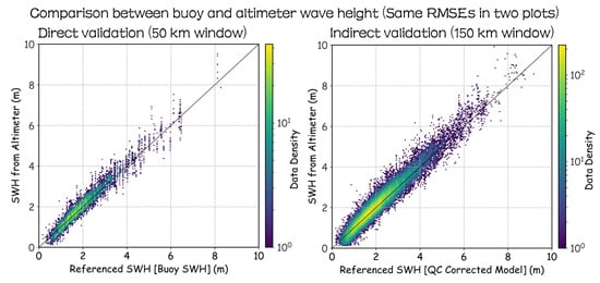
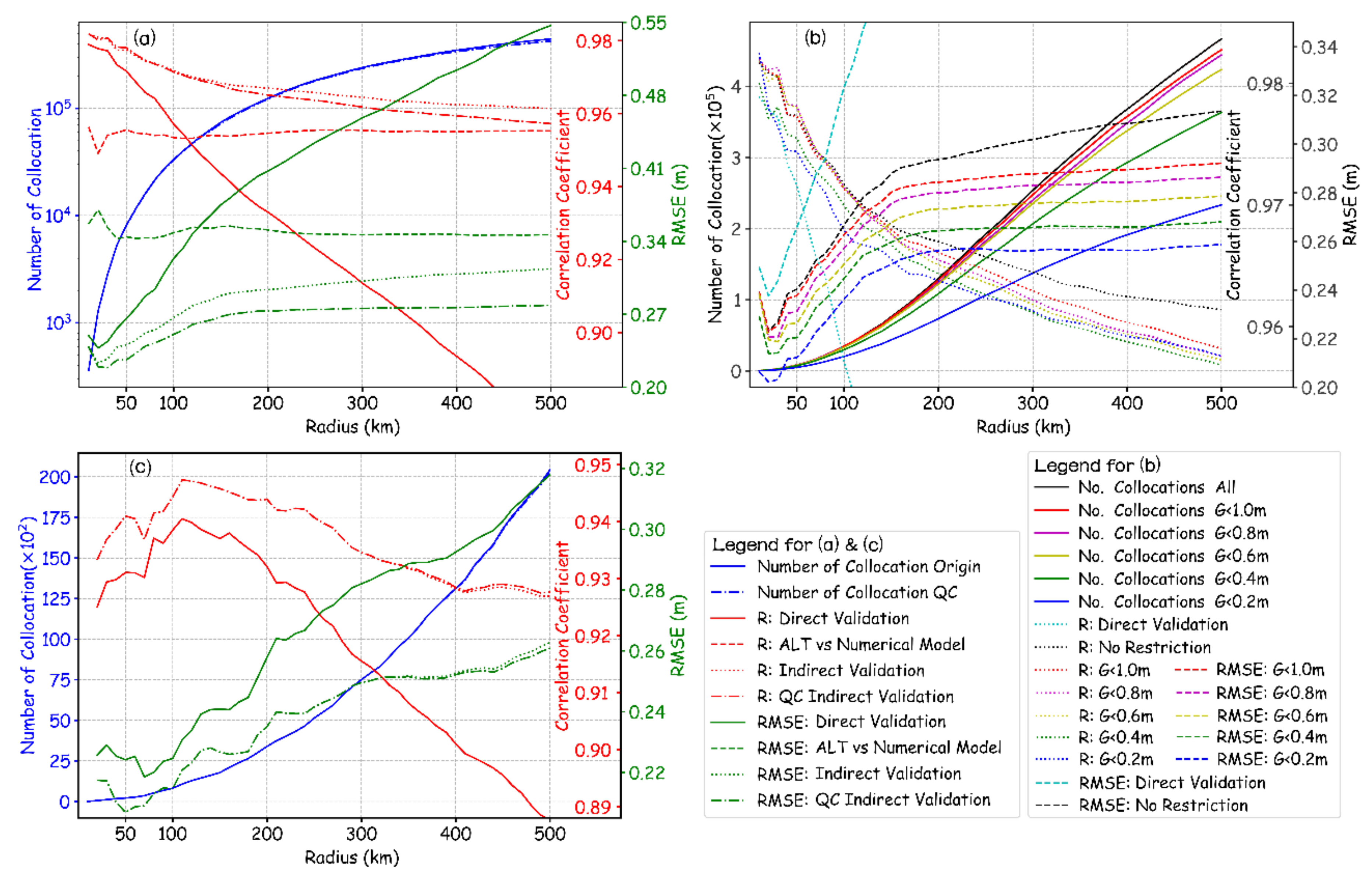
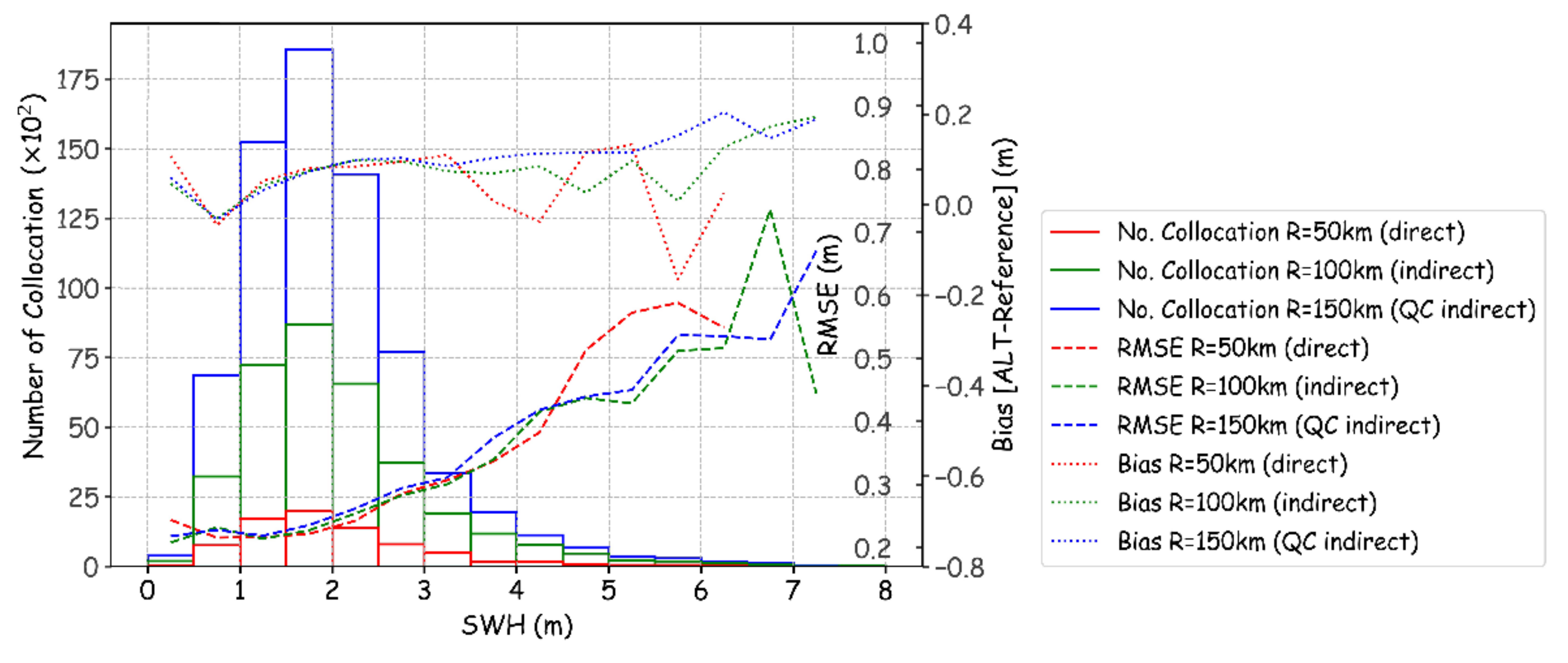
3.1. Direct/Indirect in Situ Validation

Figure 2a shows the N_col, CC, and RMSE between SWHs from Envisat and the 52 NDBC buoys as a function of the radius of the spatial window for direct in situ validation (the blue, red, and green solid lines, respectively). The N_col increases fast with the increasing radius of the spatial window. For 2011, ~8 × 10³ collocations were available with a radius of 50 km, but the N_col becomes ~3 × 10⁴/~8 × 10⁴ when the radius increases to 100/150 km. However, the RMSE/CC also increases/decreases fast with increasing radius. For example, the RMSE is 0.27 m with a radius of 50 km but becomes 0.37 m when the radius is 150 km. The RMSE between Envisat and IOWAGA SWHs is only ~0.34 m (the green dashed line in Figure 2a), indicating that using a 150-km spatial window for direct validation is even worse than using the modeled SWH as reference. Therefore, the spatial window for direct validation has to be small to limit the representativeness error.

The CC and RMSE for indirect validation are shown also in Figure 2a (the red and green dotted lines). Although the CC/RMSE still decreases/increases with the radius, the rate of this decrease/increase is much lower than the corresponding solid lines with the connection of a numerical wave model. At a radius of 50 km, the RMSE of the indirect validation is 0.25 m, which is slightly less than the 0.27-m RMSE of the direct validation with the same window. The RMSE is 0.27 m and the CC is 0.97 when the radius is 100 km, which is generally equal to the result of direct validation for a 50-km window. Even when the radius increases to 300 km, the RMSE still remains below 0.3 m and CC exceeds 0.96, which is an acceptable accuracy that is much better than if the outputs from the numerical wave model were used as reference. These results show that indirect validation can effectively increase the N_col by enlarging the spatial window while only slightly increasing the error, thus, is a better method than direct validation.

The wave model output used as a bridge here is a global hindcast with a rather coarse resolution. Such a coarse resolution is typically not good at modeling high spatial-temporal gradients of SWHs, which is usually induced by extreme events (e.g., storms) and shapes of fine-scale coastlines (e.g., island shadowing). Using a regional model with higher resolution should enable a better comparison for indirect validation. Meanwhile, a method was presented here to alleviate these problems by introducing a simple quality control (QC) parameter:

$$G=\left|M_{ref}-M_{rs}\right|$$

(8)

It was assumed to usually be difficult for the model to accurately present the SWH gradient between two spatial-temporal locations if G is large. A threshold for G can be used to exclude cases that are badly modeled. The results of the indirect validation of Envisat SWHs with different restrictions (from 0.2 m to 1.0 m with an interval of 0.2 m) of G are shown in Figure 2b. The N_col and RMSE both decrease with decreasing the threshold, which is within expectation. The CC also slightly decreases with decreasing threshold. This is because more high-SWH cases in storm events were excluded by a stricter QC, which decreased the scatter of the SWHs. A slightly lower CC does not mean worse comparison. Because it was found that the restriction of G < 0.6 m (the yellow lines in Figure 2b) can effectively decrease the RMSE without excluding many samples, it was used in the following analysis. The N_col, CC, and RMSE for indirect in situ validation after a QC of G < 0.6 m are also shown in Figure 2a as dot-dashed lines. The change of the N_col before and after the QC is negligible on a log-scale. The CC remains almost unchanged within a 150-km radius before and after the QC, while the RMSE becomes significantly lower after the QC, and almost does not increase with the radius after 200 km. This is because most collocations within 500 km are within the “buoy network” in the Northern Hemisphere. In this region, the model output can be corrected by the observations from several nearby buoys using Equation (4). Therefore, a larger spatial window can be used for indirect validation after this simple QC.

Outside this buoy network, the error still increases with the increase of collocation radius. For example, Figure 2c shows both the direct and indirect validation results of Envisat SWH using Stratus Wave Station (32012) which is the only buoy in the Southern Hemisphere (SH) in Figure 1 (the inner plot). In this case, the RMSE/CC increases/decreases with the radius for both direct and indirect validations. However, the increasing rate is slower for indirect validation than for direct validation. Indirect validation using a spatial window of 160 km has the same RMSE and a higher CC than direct validation using a spatial window of 50 km, while the N_col is increased by an order of magnitude compared with direct validation. Because there are fewer wave observations in the SH than in the Northern Hemisphere, there is a need to fully utilize the observations to validate the SWH retrievals in the SH, and indirect validation is also useful for the conditions for which few reference data are available.

Figure 2a shows that the RMSEs of 50-km-window direct validation, 100-km-window indirect validation without QC, and 150-km indirect validation QC were all about 0.27 m. To compare the three validation methods, Figure 3 shows the N_col, bias, and RMSE of Envisat SWHs for the three conditions as a function of reference SWH. The results clearly indicate that indirect validation with QC increases the N_col at all SWHs. In the SWH range of 0.5-3.5 m, all three methods give a similar error estimate. However, when SWH becomes larger, direct validation cannot provide stable estimates of the bias and RMSE using only 1-year data because of shortness of collocations. This problem can also be solved by indirect validation with more collocations at high SWHs. Even when the SWH is higher than 5 m, more than 100 collocations can still be obtained by indirect validation. The results of indirect validation with only one-year data show that the bias varies slowly with SWH and the RMSE increases almost linearly with SWH, which matches the error features of altimeter SWH derived from many years of direct validation [10], thus corroborating the strength of indirect validation.

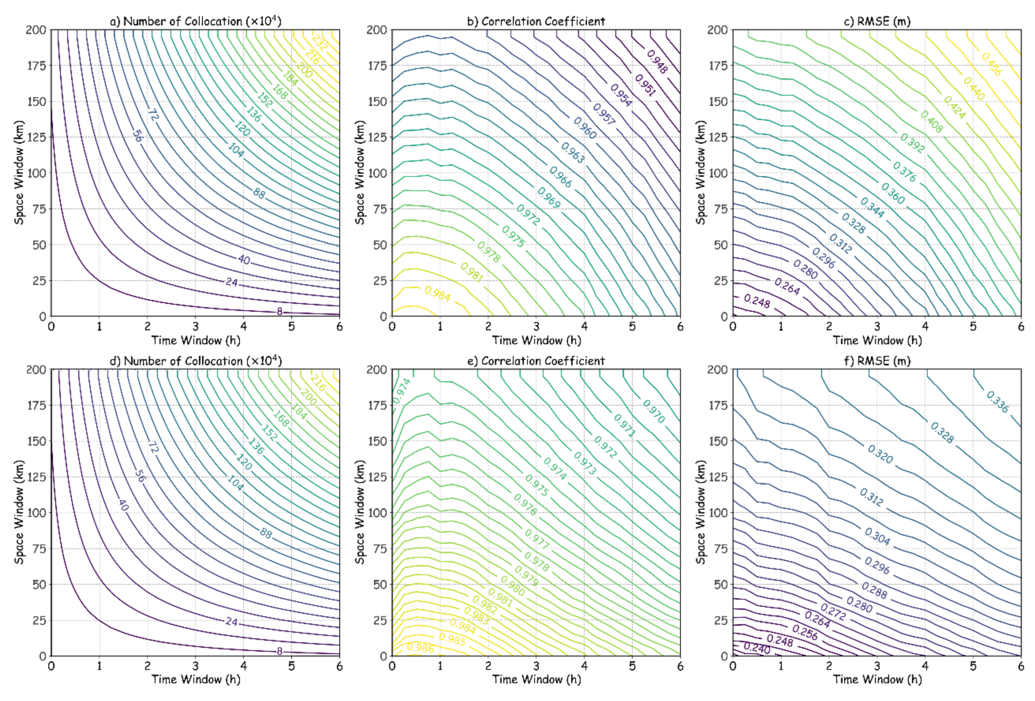
3.2. Direct/Indirect Cross Validation

Figure 4 shows the N_col, CC, and RMSE as a function of the size of the spatial-temporal window for both direct and indirect cross comparison (with a QC of G < 0.6 m) between Envisat and Jason-1 SWHs for 2011. For direct cross-validation, the results are similar to those shown in Figure 2a, indicating that the CC/RMSE decreases/increases with window size. A 30-min-50-km window corresponds to an N_col of ~8 × 10⁴, a CC of 0.980, and an RMSE of 0.284 m. However, the distributions of CC and RMSE indicate that a 30-min-50-km window might not be the optimal option. A 90-min-37.5-km window achieves the same RMSE and CC but N_col is twice as large.

For indirect cross-validation, the impact of QC on the N_col was small, as shown in Figure 4a,d, and the CC/RMSE also decreases/increases with window size. However, the gradient of CC/RMSE is smaller in Figure 4e,f than in Figure 4b,c. With an RMSE of 0.284 m, corresponding to the 30-min-50-km window of direct validation, ~2.7 × 10⁵ collocations can be obtained by indirect validation using a 120-min-50-km window. This enlarges the temporal window four times. Even if compared with the 90-min-37.5-km window, indirect validation can increase the N_col for more than 50%. Therefore, this idea of indirect validation is also helpful for cross-validation.

4. Discussion and Conclusions

After removing the systematical bias between remote sensing data and reference data, their variance can be decomposed as:

$${\sigma }^2={\sigma }_{rs}^2+{\sigma }_{ref}^2+{\sigma }_{st}^2$$

(9)

where σ_rs and σ_ref represent the random error (RMSE) of the two datasets, and σ_st represents the representativeness error induced by the difference of spatial-temporal locations of the two datasets. If the reference dataset is regarded as the “ground truth”, σ_ref = 0. In the direct validation, σ_st is also assumed to be zero so that σ_st is considered a part of σ_rs. In the indirect validation, σ_st is compensated by numerical models so that σ_st is reduced, which can be regarded as the theoretical basis to explain why indirect validation has a better performance than direct validation.

An important assumption behind indirect validation in this study is that the numerical wave hindcast is able to partly resolve the difference between the modeled values at the altimeter observation and the reference data. If the model data are completely wrong, indirect validation cannot get a better result than direct validation. After years of development, most contemporary numerical hindcasts have reasonable performance and can, at least, partly resolve this difference (e.g., [11,12]). With the improvement of numerical models, the estimated σ_st can become increasingly accurate, from which indirect validation will also benefit. For example, buoys close to coastlines are usually not used in the validation of altimeter SWH because of the seaward sampling problem (e.g.,[6]). Buoys close to coastlines are also not used in this study because the 0.5°×0.5°-resolution IOWAGA dataset is not sufficient for resolving coastal wave processes. However, if a high-resolution numerical wave hindcast is used, the coastal gradient of SWH can be considered and then many coastal buoys can also be adequately utilized by indirect validation. Applying the indirect validation method to a high-resolution model will be particularly useful for the validation of altimeter measurements in the coastal area (e.g., [13]). In [13], the numerical wave model was also involved in the validation of altimeter SWH. They used it to evaluate the co-variation between modeled values at the buoy and altimeter locations using linear regression. However, the pattern of co-variation between two points is usually complicated. For example, in the open ocean, there can be a time lag between the wave conditions at two points considering the propagation of waves, which can lead to a bad regression. However, it is known that the correlation between two points in the wave model output after shifting with the propagation time of swells can be high even if they are thousands of kilometers away from each other [14]. In coastal regions, the modulation of water depth can also lead to nonlinear co-variation between two points, which can also lead to bad linear regression. Therefore, these co-variations should be better described by simply the difference between two points in a numerical wave model.

In more advanced methods of error analysis, such as triple collocation (e.g., [15,16]), σ_ref is also not regarded as zero and the error is jointly analyzed using another independent data source (e.g., a numerical model). Another merit of the indirect validation presented here is that it is compatible with triple collocation. Although Section 3 used model data for indirect validation, the information used is only the gradient of SWH (the difference between two locations) instead of SWH itself, and SWH is generally independent of its gradient. In fact, the idea of indirect validation is very close to that of data assimilation, but only the “re-analysis” results near the reference observations were used to validate other observations. More advanced data assimilation methods, such as optimal interpolation (e.g., [17]), can be used to better consider the error of the “ground truth” (σ_ref) to obtain a better comparison. However, the method used in this study is easier to handle (no need to run a model) and can better guarantee the independence between the model output and the “assimilated” results. Therefore, information from the model can still be employed as an independent data source for triple collocation. In addition, because the indirect in situ validation can greatly enlarge the spatial window for collocation, it is even possible to triply collocate the SWH data from two altimeters and the buoys.

The key strength of indirect validation is that it can obtain more collocations than direct validation for a given error tolerance. Therefore, it can shorten the time required for preliminary data calibration and validation after the launch of a satellite. Moreover, indirect validation is particularly useful for the conditions for which few reference data are available. This study used SWHs from altimeters as an example to demonstrate the effectiveness of indirect validation. However, the method itself can be used for many different types of remote sensing systems because σ_st in Equation (9) almost always exists. Moreover, artificial intelligence is developing fast and is becoming widely used for designing empirical retrieving algorithms of ocean remote sensing. A large number of collocations are needed to train these algorithms, which can also be obtained by indirect validation. This study has shown the feasibility of indirect validation, and future studies can be conducted for detailed calibration and validation of different remote sensing systems using this method.

References

1. Steele, K.E.; Mettlach, T.R. NDBC wave data - current and planned. In Proceedings of the Ocean Wave Measurement and Analysis - Proceedings of the Second International Symposium, New Orleans, LA, USA, 25–28 July 1993; pp. 198–207. [Google Scholar]
2. Monaldo, F. Expected differences between buoy and radar altimeter estimates of wind speed and significant wave height and their implications on buoy-altimeter comparisons. J. Geophys. Res. Ocean. 1988, 93, 2285–2302. [Google Scholar] [CrossRef]
3. Ribal, A.; Young, I.R. 33 years of globally calibrated wave height and wind speed data based on altimeter observations. Sci. Data 2019, 6, 77. [Google Scholar] [CrossRef] [PubMed] [Green Version]
4. Liu, Q.; Babanin, A.V.; Guan, C.; Zieger, S.; Sun, J.; Jia, Y. Calibration and Validation of HY-2 Altimeter Wave Height. J. Atmos. Ocean. Technol. 2016, 1, 919–936. [Google Scholar] [CrossRef] [Green Version]
5. Zhang, H.; Wu, Q.; Chen, G. Validation of HY-2A Remotely Sensed Wave Heights against Buoy Data and Jason-2 Altimeter Measurements. J. Atmos. Ocean. Technol. 2015, 2, 1270–1280. [Google Scholar] [CrossRef]
6. Durrant, T.H.; Greenslade, D.J.M.; Simmonds, I. Validation of Jason-1 and Envisat Remotely Sensed Wave Heights. J. Atmos. Ocean. Technol. 2009, 26, 123–134. [Google Scholar] [CrossRef]
7. The WAVEWATCH III Development Group. User Manual and System Documentation of WAVEWATCH III version 5.16. 2016. Available online: https://polar.ncep.noaa.gov/waves/wavewatch/ (accessed on 16 June 2020).
8. Ardhuin, F.; Rogers, E.; Babanin, A.V.; Filipot, J.-F.; Magne, R.; Roland, A.; van der Westhuysen, A.; Queffeulou, P.; Lefevre, J.-M.; Aouf, L.; et al. Semiempirical Dissipation Source Functions for Ocean Waves. Part I: Definition, Calibration, and Validation. J. Phys. Oceanogr. 2010, 40, 1917–1941. [Google Scholar] [CrossRef] [Green Version]
9. Rascle, N.; Ardhuin, F. A global wave parameter database for geophysical applications. Part 2: Model validation with improved source term parameterization. Ocean Model. 2013, 70, 174–188. [Google Scholar] [CrossRef] [Green Version]
10. Queffeulou, P.; Ardhuin, F.; Lefèvre, J.-M. Wave height measurements from altimeters: Validation status and applications. In Proceedings of the OSTST Meeting, Ocean Surface Topography Science Team, San Diego, CA, USA, 19–21 October 2011; pp. 19–21. [Google Scholar]
11. Liu, Q.; Rogers, W.E.; Babanin, A.V.; Young, I.R.; Romero, L.; Zieger, S.; Qiao, F.; Guan, C. Observation-Based Source Terms in the Third-Generation Wave Model WAVEWATCH III: Updates and Verification. J. Phys. Oceanogr. 2018, 49, 489–517. [Google Scholar] [CrossRef]
12. Cavaleri, L.; Alves, J.-H.G.M.; Ardhuin, F.; Babanin, A.; Banner, M.; Belibassakis, K.; Benoit, M.; Donelan, M.; Groeneweg, J.; Herbers, T.H.C.; et al. Wave modelling - The state of the art. Prog. Oceanogr. 2007, 75, 603–674. [Google Scholar] [CrossRef] [Green Version]
13. Nencioli, F.; Quartly, G.D. Evaluation of Sentinel-3A Wave Height Observations Near the Coast of Southwest England. Remote Sens. 2019, 11, 2998. [Google Scholar] [CrossRef] [Green Version]
14. Jiang, H.; Mu, L. Wave climate from spectra and its connections with local and remote wind climate. J. Phys. Oceanogr. 2019, 49, 543–559. [Google Scholar] [CrossRef] [Green Version]
15. Stoffelen, A. Toward the true near-surface wind speed: Error modeling and calibration using triple collocation. J. Geophys. Res. Ocean. 1998, 103, 7755–7766. [Google Scholar] [CrossRef]
16. Caires, S.; Sterl, A. Validation of ocean wind and wave data using triple collocation. J. Geophys. Res. Ocean. 2003, 108. [Google Scholar] [CrossRef]
17. Hersbach, H.; Bell, B.; Berrisford, P.; Hirahara, S.; Horányi, A.; Muñoz-Sabater, J.; Nicolas, J.; Peubey, C.; Radu, R.; Schepers, D.; et al. The ERA5 global reanalysis. Q. J. R. Meteorol. Soc. 2020, 146, 1999–2049. [Google Scholar] [CrossRef]
Figure 1. The locations of the 51 National Data Buoy Center (NDBC) buoys (red dots) used in the study. The inner subplot shows the location of buoy 32012. A few buoys could be redeployed during the study period. The color indicates the distance of an oceanic point to its nearest buoy. Distances exceeding 1000 km are not shown, and distances are also not shown if the great circle connecting two points is blocked by land.
Remotesensing 12 02627 g001
Figure 2. The Ncol, correlation coefficient (CC), and root-mean-square-error (RMSE) of Envisat significant wave heights (SWHs) versus buoy SWHs as a function of the radius of the spatial window. In subplot (a), each color represents a parameter and each type of line represents a type of validation: blue, green, and red lines represent Ncol, RMSE, and CC, respectively; the solid, dotted, dot-dashed, and dashed lines represent the results of direct validation, indirect validation without and with a quality control (QC) of G < 0.6 m, and the direct comparison between IOWAGA and Envisat SWHs, respectively. In subplot (b), each color represents a QC standard for indirect validation and each type of line represents a specific type of validation: The solid, dashed, and dotted lines represent Ncol, RMSE, and CC, respectively; the cyan, black, and other color lines represent the results of direct validation, indirect validation without QC, and indirect validation after a QC with different values of G. Subplot (c) is the same as (a), but only the data from buoy 32,012 was used.
Remotesensing 12 02627 g002
Figure 3. The Ncol, CCs, and RMSEs of Envisat SWHs as a function of reference SWH. Each type of validation is represented by a different color. Red: direct validation; Green: indirect validation without QC; Blue: indirect validation with a QC of G < 0.6 m. The overlaid histograms show the number of collocations, dashed lines show RMSEs, and the dotted lines show the bias at each SWH bin (0.5 m interval).
Remotesensing 12 02627 g003
Figure 4. (a,d) Ncol, (b,e) CCs, and (c,f) RMSEs of Envisat SWHs versus Jason-1 SWHs as a function of the size of the spatial-temporal window. The upper row shows the results of direct cross-validation and the lower row shows the results of indirect cross-validation with a QC of G < 0.6 m. The color scales of the contours are identical for the same parameters.
Remotesensing 12 02627 g004