Abstract
An analysis of almost 200 references has been carried out in order to obtain knowledge about the DEM (Digital Elevation Model) accuracy assessment methods applied in the last three decades. With regard to grid DEMs, 14 aspects related to the accuracy assessment processes have been analysed (DEM data source, data model, reference source for the evaluation, extension of the evaluation, applied models, etc.). In the references analysed, except in rare cases where an accuracy assessment standard has been followed, accuracy criteria and methods are usually established according to the premises established by the authors. Visual analyses and 3D analyses are few in number. The great majority of cases assess accuracy by means of point-type control elements, with the use of linear and surface elements very rare. Most cases still consider the normal model for errors (discrepancies), but analysis based on the data itself is making headway. Sample size and clear criteria for segmentation are still open issues. Almost 21% of cases analyse the accuracy in some derived parameter(s) or output, but no standardization exists for this purpose. Thus, there has been an improvement in accuracy assessment methods, but there are still many aspects that require the attention of researchers and professional associations or standardization bodies such as a common vocabulary, standardized assessment methods, methods for meta-quality assessment, and indices with an applied quality perspective, among others.
1. Introduction
Digital Elevation Model (DEM) is a generic term for digital topographic and/or bathymetric data, in all its forms [1]. There is some confusion in the use of the terms DEM (Digital Elevation Model), DTM (Digital Terrain Model), and DSM (Digital Surface Model). We are going to consider that the term DSM is a case of DEM in which the elevations contemplate the buildings, vegetation, etc., that is, all the elements on the earth’s surface. The term DTM would be a model in which the elevations are referred to the bare ground. DEM is a generic term that would encompass both terms. Although the terms DEM and DTM can be equalized, a DEM can be considered a subset of a DTM, since these can represent other morphological elements [1].
Several data models are considered to store the elevation of the terrain, e.g., regular spaced tesellation (grids), regular spaced points mesh (lattice or mesh of points), Triangular Irregular Network (TIN), curves of iso-elevation (contour lines), etc. [1]. We are going to deal with the first one as it is currently the most widely used for DEMs treatment [2]. Grid models are conformed as a regular-rectangular array of cells each of which stores an attribute value, so the area of each cell adopts the same elevation value, producing a sudden change in the limits of each cell (a raster model). The elevation is represented by patches, which are the cells of the grid. Thus, the size of the cell, or resolution, is a key parameter. This parameter is related to the traditional concept of scale and detail of cartographic products. Small cell sizes, giving high spatial resolution, are linked to large scales and great spatial detail. Large cell sizes, giving small resolution, are linked to small scales and less spatial detail. Therefore, there is a direct relationship between resolution and accuracy: the higher the resolution, the greater the expected accuracy, and vice versa. In fact, there are many studies that empirically show that increasing the size of the cell decreases the accuracy of the DEM [3]. Finally, one of the main practical advantages is the amount of existing software tools for working with grid models; this is because they are easy to handle, data are arranged in the form of a regular array (a matrix). This arrangement facilitates the design of algorithms for working with this type of data, unlike the Irregular Triangle Networks (TIN) in which the data are scattered and random. A matrix is a fast and efficient data structure for the analysis of algorithms and as primary surface representation for analysis [1].
Data capture technologies (e.g., field survey [4], photogrammetry [5], remote sensing [1,6], LiDAR (Light Detection and Ranging) [7], etc.) have a great relevance for DEM production and quality. In our view, in recent years, there have been two fundamental advances—on the one hand, modern techniques such as LiDAR determine elevation by direct distance measurement procedures, which offers much more accuracy in elevation determination; and on the other hand is the ability to generate global DEM products (known as GDEM) (e.g., SRTM—Shuttle Radar Topography Mission-, ASTER—Advanced Spaceborne Thermal Emission and Reflection Radiometer-, TanDEMx-TerraSAR-X add-ons for Digital Elevation Measurement-) with great ease and accuracy. DEMs are geospatial data products that are mostly produced by national mapping agencies (e.g., the Instituto Geográfico Nacional in Spain, the Ordnance Survey U.K., etc.) and in most developed countries, the territory is covered with high-spatial resolution DEMs. DEMs are data products at the service of entrepreneurship, public administrations, the private sector, researchers, and universities, etc. in order to generate added value [8].
DEMs are data products with applications in an extensive set of disciplines such as Civil Engineering [9], Hydrology [10], Geomorphology [11], Biology [12], etc. Some of their applications include modelling for the prevention of natural disaster (floods [13], fires [14], etc.), soil erosion studies [15], weather forecasting [16], climate change [17], etc. DEMs have been included as a data theme for Europe (Inspire) and as a global fundamental geospatial data theme by the United Nations Committee of experts on global geospatial information management [18]. Therefore, one of the fundamental premises is the need for DEMs to have sufficient quality to meet the needs of those applications [19]. It could be the case that a DEM with a certain quality level is used in a study that requires a different quality level. Two cases can occur: First, that we use a DEM with a higher level of detail and accuracy than the needs of the study require, so we would be missing the possibilities of DEM and consuming more resources (e.g., memory and hard disk space, computation time, etc.). Secondly, that we use a DEM with an insufficient level of detail and accuracy for the needs of the study, so we would be conducting a study generating inaccurate results, which may lead to erroneous conclusions. In order to solve this problem, users should know the quality of the DEM product they want to use, which must be recorded in the product’s metadata. However, it has been verified [2] that users of DEMs are not aware of the importance of knowing the quality of the DEM used before using it in their studies or analysis. The quality of a geospatial data product covers a broad range of aspects (e.g., positional, thematic, temporal, logical, etc.) [2] from the producer’s perspective. From the user’s perspective, quality should adopt a character more relevant to the specific application and use case that is intended to be developed, which is related to the “fitness for use” perspective on quality.
To the best of our knowledge, there are no standardized methods for the quality assessment of DEMs with an integral vision or centered on the “fitness for use” perspective; however, there are many methods of assessing (positional) accuracy that can be applied to DEMs. These methods have evolved from the NMAS (National Map Accuracy Standard) [20] to the most recent, complex, and sophisticated: the ASPRS Positional Accuracy Standards for Digital Geospatial Data [21]. In this way, we must indicate that in this paper we use “quality assessment” and “accuracy assessment” to refer to the same idea: in both cases, we refer to the discrepancy between elevations as defined in Section 2 (altimetric accuracy). We must bear in mind that when we talk about quality in a DEM, despite the fact that the quality concept is much broader and covers more aspects of a data product, we assimilate it to the altimetric accuracy of the DEM since this is the main data that DEMs provide us with.
The aim of our work is to analyse the methods used for the accuracy assessment of DEMs in the last three decades. Accuracy assessment methods usually give a final value (or values) as the accuracy parameter of the DEM, and the procedure for obtaining this value of accuracy is what we intend to investigate. We must also indicate that our objective is to analyze how a cartographic product that we assume is ready for use is evaluated, that is, it is the producer who has previously been in charge of filling out, completing and preparing a product for use by users. To achieve this purpose, an analysis of almost 200 references has been carried out. In the analysed references, except in rare cases that an accuracy assessment standard has been followed, accuracy criteria and methods are usually established according to the premises established by the authors. Our aim will be to present an overview of the methods used and criteria followed for the DEMs’ accuracy assessment over the established period of time. We believe that this analysis can be of great interest to both producers and users as it offers a broad overview of relevant aspects that can help them improve their assessment methods and report (e.g., metadata) on the accuracy of DEMs. In this way, a more rational use of resources could be made and, on the other hand, an appropriate use of DEMs would be made, adapting the analysis to their possibilities based on their accuracy.
This document is organized as follows: After this introduction (Section 1), an approximation to the concept of vertical accuracy is presented (Section 2). Next, the procedures followed to compile the references and a brief bibliographic analysis of them will be presented (Section 3). Structured in eleven subsections, the fourth section presents the results and an analysis of them (Section 4). Finally, a discussion and general conclusions focused on the most relevant aspects are presented (Section 5).
2. Approaching Vertical Accuracy in Digital Elevation Model
According to ASPRS (American Society for Photogrammetry and Remote Sensing) [22], vertical accuracy is the main criterion in the specification of the quality of elevation data. Nevertheless, the horizontal accuracy in a DEM is of great importance as well, since horizontal accuracy has a great influence on vertical accuracy [22,23]. However, in the case of DEM products, it is not usual to inform about horizontal accuracy.
When talking about the accuracy of a DEM, two types of accuracies can be distinguished [1,23,24]: absolute and relative vertical accuracies. The absolute vertical accuracy is the vertical accuracy with respect to a Geodetic-Cartographic Reference System where an official altitude Datum has been adopted. On the other hand, the relative vertical accuracy refers to the accuracy with respect to a local reference system. Absolute accuracy is necessary for the integration of altimetry data in frames relative to large areas of interest (e.g., a province, a region, a nation, etc.). Relative accuracy is only suitable for very local analyses and is more related to parameters derived from the neighborhood (e.g., slope and aspect calculations).
The vertical accuracy of a DEM means the accuracy in the elevation obtained at any location in the DEM. This vertical accuracy is related to the discrepancies d obtained from the comparison of the elevation hDEM of the DEM product evaluated in a specific location i, against the elevation hREF obtained from a source of greater accuracy in the same location i. Following Florinsky (1998) [25], we do not use the term error here because this term is not adequate since the reference values used in the comparison are also affected by their own uncertainty. In the same way, the “Guide to the Expression of Uncertainty in Measurement” [26] indicates that the “absolute error” is not considered measurable or estimated, discouraging the use of this term since the real value cannot be known in any way. We can determine a given value closer to the actual than another, but taking into account all the factors that influence the determination of a measure any value will always be affected by uncertainty, and therefore the true value is never known. However, we will consider as true value that which is of greater accuracy than the one evaluated. Accuracy is related to the statistical difference between the value considered as true and the value observed. The true actual value is approximated by the source of greater accuracy (the reference); this is an exigency in order to minimize the influence of the uncertainty of this value hREF into to the accuracy estimation of hDEM. Usually “at least three times” greater accuracy is considered [20,22]. Accuracy refers to the population, in a statistical sense, of those discrepancies and means how close the DEM recorded value (measured) is to the actual value. Accuracy comprises trueness and precision, as stated by ISO 5725-1 [27]. Trueness is the absence of bias, and precision is a measure of dispersion. This model is adequate for normally distributed discrepancies where the displacement parameter (µ) is the bias, and the shape parameter (σ) is the precision. Butler (1998) [28] established definitions for precision, reliability, and accuracy related to DEMs. Precision is related to random errors of data sources (Ground Surveying, Photogrammetry, LiDAR, etc.); reliability is related to outliers in measurements or elaboration processes, and finally accuracy is related to systematic errors (e.g., ignoring the effects of lens distortion in photogrammetry).
The following equations give us the value of the elevation discrepancies at any point i, the mean of all these discrepancies, the standard deviation, and the RMSE:
where
- hDEM,I elevation in position i of the DEM product
- hREF,I elevation in position i of the reference
- di discrepancy in elevation in position i
- n number of samples
- µd mean value of discrepancies
- σd standard deviation of discrepancies
- RMSEd root mean squared error of discrepancies
Therefore, we could consider a DEM accurate if the mean and standard deviation of the discrepancies are low values. In most cases, the RMSEd is used as a parameter to express the vertical accuracy of a DEM. The RMSEd coincides with the standard deviation σd only when the bias is null (µd ≈ 0); otherwise, the RMSEd is a compound parameter of both of them, and is more adequate for non-normally distributed data. In most of the studies, as we will see and analyze later, the differences in elevation are considered with a normal distribution behavior. However, there is an increasing number of studies considering a non-normal distribution. This is related to data capture technology. Thus, for example, the data from Photogrammetry often have errors with a normal behavior, and the data from LiDAR do not have a normal distribution [1]. In this way, the description of accuracy using a single parameter is not possible in many cases due to the large number of outliers. It therefore suggests that robust error distribution descriptors (minimum, maximum, median, quartiles, interquartile range, deciles, etc.), be used in addition to the conventional descriptors.
The discourse presented in the previous paragraphs is based on statistics and is closely related to the production processes of DEM, so it is something that DEM producers must know and adequately manage. However, the users’ perspective is quite different. Many users do not fully understand the accuracy and its parameters [29] and would need the quality to be expressed in a way closer to their interests (fitness for use). Unfortunately, to the best of our knowledge, an adequate framework for this purpose has not been developed, although some cases related to this objective are presented in Section 4.1.1.
3. Materials and Methods
This section covers the materials and methods employed in our analysis. First, the method applied to collect the bibliographic material (references) will be presented, followed by a bibliographic analysis of this material.
3.1. Method for the Selection of References
In order to obtain adequate material for our review of the procedures used for the quality assessment of DEM, some previous decisions were taken:
- We decided the typology of the materials to consider in our analysis: standards, scientific papers, PhD Theses, relevant reports, and congress publications.
- We tried to ensure that all the documents selected had a certain scientific guarantee, and for this reason, we will select papers published in scientific journals (e.g., included in the Journal Citation Report); contributions to international congresses of recognized prestige; and reports about DEM quality evaluations elaborated by cartographic institutions of international scope.
- We decided on a 30-year temporal window for the general analysis (1990–2019). An exception has been considered here in the case of standards and their guidelines until 1947 in order to include the NMAS [20], which had a high level of application until the end of the 1990s [30]. The period of time selected is intended to provide a broad view of the studies carried out in relation to our topic. In this way, we cover a wide period of time in which technological change has taken place, both in means of capturing information and in the technologies and computer means (software and hardware) for processing DEMs. This would show us how the methods used in the quality evaluation of DEMs have evolved, as well as the considerations taken into account at each moment.
- We establish a set of key words (DEM, assessment, quality, accuracy) for the searches in titles and abstracts.
We carried out the searches on different platforms in order not to present views biased by any of them; thus, our search included scientific databases such as ScienceDirect and Scopus, in doctoral thesis search engines such as Dart-Europe, OATD (Open Access Theses and Dissertations) and NDLTD (The Networked Digital Library of Theses and Dissertations) and Google Scholar.
The selection of documents has followed the following criteria as fundamental:
- Studies that deal directly with the accuracy assessment of DEMs
- Studies that deal with the modeling of the spatial distribution of DEM accuracy
- Studies that deal with the use of different statistics to express DEM accuracy
- Studies on the prediction of DEM accuracy from mathematical models
- Studies in which the accuracy assessment they are based on is related to the interpolation method used to obtain the DEM
- Studies that try to relate the accuracy of the DEMs obtained by varying some parameters of the obtaining procedure (e.g., depending on the number of control points used in the photogrammetric restitution process or using other homologous image settings)
- Comparisons between different DEMs with different cell size and altimetric accuracy Considering one of the models as a reference
- Comparisons between different DEMs depending on the capture technology used
- Studies in which the accuracy of the DEMs is a function of the morphological parameters of the land, for example slope and roughness
- Studies that assess the accuracy of the DEM based on the accuracy obtained in derived morphological parameters such as slope, aspect, etc.
- Studies in which the quality or accuracy of the DEM is related to specific use cases (e.g., in hydrology: catchment areas, drainage network studies, etc.)
3.2. Bibliographic Analysis of the References
Finally, a total of 173 documents have been reviewed. Scientific Articles, Congress Publications, Standards, Reports, and Doctoral Theses have been considered (Table 1). The 122 scientific papers reviewed were obtained by the search conducted in scientific journals, most of them indexed in the Journal Citation Report (JCR). The rest of the studies reviewed have been compiled through different searches in the internet (Google Scholar, etc.) There is only a small percentage (6%) that corresponds to non-JRC-indexed documents.

Table 1.
Types and number of documents reviewed.
As mentioned above, the time window chosen for the analysis runs from 1990 to 2019. Figure 1 shows the number of documents for each year in this interval, where standards have been eliminated from this figure. Figure 1 shows that there is an incremental tendency for the number of documents from 1990 to approximately 2012. Between years 2010 and 2016, there is a peak with a large number of cases, and afterwards a decrement. We consider that this decrement in more recent years is due to a change in the accuracy perspective developed in scientific papers. Studies related to a “fitness-for-use” quality assessment perspective of DEMs are emerging and occur more frequently than those that simply analyze production methods and DEM quality.
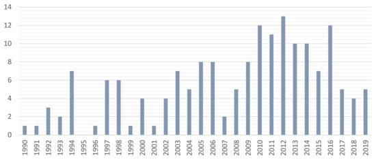
Figure 1.
Temporal distribution of the number of documents reviewed.
In relation to standards and guidelines, Table 2 lists those taken into consideration in our analysis. Most of the documents are standard, but four guides have also been included, as these in many cases are highly explanatory. The standards are mostly of American origin, either from official bodies (e.g., FGDC—Federal Geographic Data Committee) or professionals (e.g., ASPRS—American Society for Photogrammetry and Remote Sensing). We highlight the Spanish standard UNE 148002 given that it presents a totally different framework for geospatial data control and that it is based on ISO 2859 parts 1 and 2.
Table 2.
Standards Reviewed.
The distribution by country of all the documents reviewed (173) is widely dispersed throughout all continents. More studies are carried out in more developed countries than in developing countries, which seems entirely logical. The country with the highest percentage of reviewed studies is the U.S.A. with 16.18%. We observe that there are several studies at a global level and a smaller number at a continental level. In our corpus, we only reviewed studies at the continental level in South America, Europe, and Antarctica, and several globally. These studies of very broad scope are recent studies in which we highlight the possibility of using GDEM, thanks to the availability of access to open data from these models (e.g., SRTM, ASTER).
4. Results and Analysis
We consider relevant aspects all those related to characterizing a DEM to be evaluated and the reference data, the extension of the quality evaluation area, the type of evaluation elements used, the sample size, etc. Many of these relevant aspects are those that, in some way, should be considered in a well-established evaluation method. In order to organize them properly, this section is divided into 11 subsections that have a certain logical order, which ranges from the product to be evaluated and the source to be used to other aspects to consider, including the size of the area and the sample, etc.
4.1. Descriptive Results of the Data Used
In this section, we are going to characterize the data used in the different studies reviewed. We will describe both the DEMs evaluated and the data used for reference. We will also describe in more detail the type of grid model used and the area extensions of the works, as well as their relationship with the grid size of the models used and the data source.
4.1.1. Source of the DEM Assessed
One of the most relevant aspects of a product to be assessed is its own data source; here, that means which DEM-data-capture procedure has been used. Figure 2 represents the percentage of cases when considering eleven different DEM data sources based on technologies and available databases. We must notice that Figure 2 shows a mix of geomatics sciences, technologies, and other specific technologies for data capture, and this is due to the fact that we consider all of them relevant because of the number of occurrences. Although we initially established a higher number of classes, later we grouped some capture sources because there was a great dispersion (e.g., all satellite-image based sources such as IKONOS images, WorldView-2, etc., have been grouped into Stereophotogrammetry). Additionally, some classes are considered relevant and not grouped. This is the case of the GNSS (Global Navigation Satellite Systems, e.g., GPS) class, which is too significant to be included in a more general class called “Ground Surveying”, since the last can include other surveying methods and devices. Finally, it should be noted that 5% of documents do not explicitly detail any source and these appear as “not shown”.
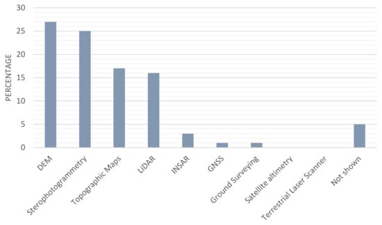
Figure 2.
Percentage distribution of DEMs (Digital Elevation Models) sources.
Figure 2 shows that the category with the most frequency of cases (26.70%) is the one that refers to existing DEMs. It may seem contradictory that the source of a DEM is a DEM. These are studies in which some of the following situations may occur:
- Studies in which the accuracy of a new version of a global DEM is evaluated (SRTM, ASTER, etc.)
- Studies in which the accuracy of a derived model (slopes, aspect, etc.) is evaluated with the use of different DEMs from national or global mapping agencies
- Studies using DEMs facilitated by national mapping agencies. Usually the DEMs provided by the mapping agencies have different sensors or sources of origin for their training
All of these cases have been grouped into the “DEM” class. In this class, 32.20% belong to ASTER GDEM, 28.81% belong to SRTM, and 15.25% belong to TanDEM-X, these being the three with the highest percentage with respect to the others.
Secondly, there are the DEMs elaborated from stereoscopic images, from aerial and space platforms. Thirdly, topographic maps stand out in this analysis because they were one of the most widely used DEM-data sources in the first decade of our analysis (Figure 3). Recently, the number of cases that use the LiDAR, TLS (terrestrial laser scanning), and INSAR (interferometric synthetic aperture radar) is increasing. Ground Surveying and GNSS techniques are not very representative, due to the amount of time and financial resources required to prepare a DEM using these techniques, and especially if the DEM extension is large.
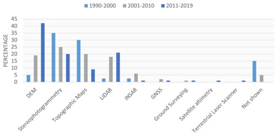
Figure 3.
Temporal distribution of the percentage distribution of DEMs sources.
Since there are currently very interesting DEM data capture technologies (e.g., LiDAR) and since there has also been a highly relevant source such as printed maps in the past, it is interesting to analyze whether the corpus of documents used reflects this situation. In this line, Figure 3 is presented. A trend observed in the last decade is the increasing use of existing DEM products. We consider that this is due to the increase of free products, especially GDEMs such as SRTM, ASTER, TanDEM-X, etc. The use of GDEMs enables the development of environmental, planning, and infrastructure projects at the national or regional level, even internationally, and they are also a very useful tool in developing countries with a poor official geospatial data infrastructure. This is also due to the moderate spatial resolution they have, in some cases reaching even 12 × 12 m. Figure 3 also shows the increase in the use of LiDAR technology but the opposite occurs with the use of printed maps where, as is logical to think, the trend of use is decreasing. Another interesting trend to highlight is the decrease in the use of Stereophotogrammetry. Cases incorporating the other alternatives are too few to establish trends.
Finally, it should be noted that sometimes the original data sources are supplemented with auxiliary data (e.g., break lines) to improve the quality of the DEM to be generated. These auxiliary data are usually vector-type and are “burned” on the grid model. In this way, 3.82% of cases (Figure 4—Row I) include fundamental lines of the terrain to improve the DEM’s accuracy and, therefore, its quality parameters [38,39]. Generally, it is about including in the model stream lines (stream burning), dividing lines, and singular points. Bonin [39] emphasizes the improvement of the quality of the DEM by including these lines since the tendency of DEM data is to underestimate the elevations in the divisions and to overestimate it in the channels. This procedure also improves the subsequent calculation of other parameters such as the slope. Some studies [39,40,41,42] analyze the effects that inclusion of these lines has on the final accuracy of the model.
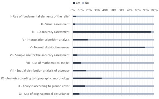
Figure 4.
Distribution of percentages of the studies analyzed that meet various considerations in the accuracy assessment of studies in which visual assessment is carried out.
Figure 4 shows more aspects considered when evaluating the quality of a DEM, in addition to the aspect considered in the previous paragraph. Therefore, from now on, we will refer to this figure on several occasions when we analyze the different aspects that are reflected in it.
4.1.2. Data Model of the Product
As stated in Section 1, it is clearly shown that most of the cases use grid models (91%), while the use of TIN models is residual (4%). In a previously-published [2] study in which a survey on DEM users is presented, 91.2% used the Grid model, a percentage that coincides with that obtained in this study. It is interesting to evidence here that the use of the contour lines is also residual because this data model was used as an intermediate data model for the capture of contour lines from printed maps to a later conversion to a grid, and is only used by very specific software tools related to civil engineering. Given its quantitative importance, more details regarding the grid model will be analyzed below.
- The grid data model
In relation to the grid model, Figure 5 shows the distribution of grid resolutions in the subset of documents where it has been indicated. In this distribution, the peak corresponding to the majority of cases (30 m resolution) splits the distribution into two parts—on the left, the resolution categorises with more presence, and on the right with less presence. This situation seems obvious given that the quantitative control of the higher resolution models is more interesting than that of the lower resolution models.
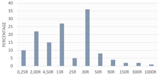
Figure 5.
Percentage distribution of grid resolutions (in meters).
There are many studies where the DEM accuracy is analyzed in relation to the grid resolution [42] in order to study its relation to the DEM’s accuracy, or to obtain the most suitable grid resolution for a given application. They start from an original DEM and then it is re-sampled to different larger grid resolutions. In some cases, derived parameters (e.g., slope or aspect) are calculated and assessed. Based on the variations of the grid resolution, 23.49% of cases use this analysis. The result is always that the larger the grid size, the lesser the accuracy, which is something that seems quite obvious [43].
Finally, in relation to the grid’s resolution, it could be considered whether or not there is a relationship between it and the extension of the area assessed. In this regard, the scatter plot of Figure 6 shows a point cloud without a clear trend, although it is hinted very slightly that the larger the study area, the larger the grid size. The large storage and information processing capabilities available today perhaps make this not overly critical. In addition, there are several cases of resolutions (e.g., 10 × 10 m, 30 × 30 m or 90 × 90 m) with application in the most varied extensions, from national territories to a few km2. We consider that this is due to the fact that these resolutions (e.g., 30 × 30 m and 90 × 90 m) correspond to some global and open-access DEMs used in numerous studies.
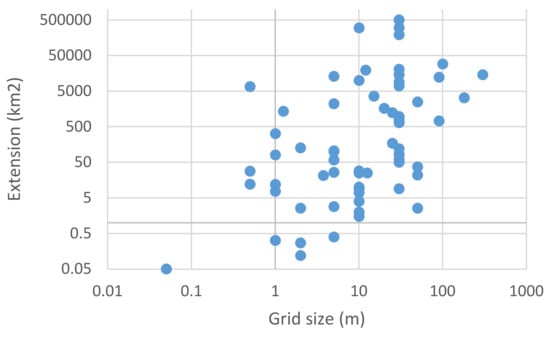
Figure 6.
Log-log representation of the relationship between extension (Km2) and grid size (m).
4.1.3. Source of the Reference Data
The source of the reference data of greater accuracy is of great relevance in this analysis since it conditions the accuracy of these data, which, as indicated, must be at least three times more accurate than the data of the product being evaluated. These sources may be existing products (e.g., a topographic map or a DEM product from an official source, etc.), but in many cases, an ad hoc survey is also carried out (e.g., a GNSS survey). Figure 7 shows the percentage distribution for the reference data sources in the corpus analyzed. In this case, it is striking how the GNSS techniques are the most widely used to obtain reference data in evaluating the quality of DEMs. Obtaining data from large-scale topographic maps is the second preferred option. Classical survey topographic methods, LiDAR, existing DEM (Figure 7), and stereophotogrammetry are options with more or less the same global relevance in the period analyzed. As previously discussed in Section 4.1.1, the “DEM” class groups all DEMs provided by mapping agencies, both national and global, which are supposed to be more accurate than the assessed DEM. It is worth mentioning the prominent use of an altimetric database, the GEDTF (Global Elevation Data Testing Facility).
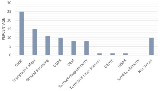
Figure 7.
Percentage distribution of reference data sources.
In relation to the temporal evolution of the use of these sources, Figure 8 shows the percentages for each of the three decades. Many of the trends shown are parallel to those indicated in Section 4.1.1 for product data sources. Specifically, the decrease in the use of printed maps and stereophotogrammetry and the increase in the use of LiDAR techniques and DEM products are evident. Another relevant aspect is that the use of GNSS techniques has an upward trend.
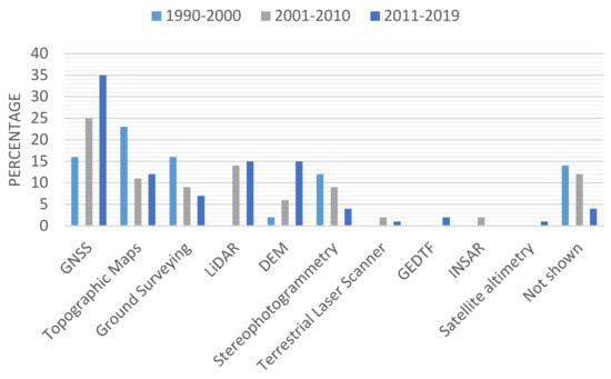
Figure 8.
Temporal percentage distribution of reference data sources.
It should be noted that some of the documents analyzed do not use a source with greater accuracy, but one with an accuracy approximately equal to the one evaluated. Another necessary requirement for an accuracy assessment to be correct is that this source be independent from the one that generated the product [37]. Although this is usually true, this aspect is not always highlighted in the references analyzed.
4.1.4. Extension of the Accuracy-Assessment Area.
Only a hundred of the revised documents explicitly reflect the extension of the accuracy-assessment area. In many cases, this data is omitted and in other cases it is not appropriate because of the nature of the document itself (e.g., standards). Figure 9 shows the distribution of cases using six extension classes: global, national, >200 km2, (25, 200] km2, (1, 25] km2, ≤1 km2). These intervals are due to the work scales which, in the authors’ opinion, are more frequent according to the objective of the study [44]. Therefore, building or civil engineering works of a local scope would be those of less than 1 km2. Urban planning, territorial planning, civil, and engineering works of a larger extension would be all those between 1 and 25 km2. Territorial planning works, large civil engineering and environmental studies, hydrological, geological analysis, etc., would be those included in extensions between 25 and 200 km2. Finally, all those studies on environmental impact, hydrology of extensions larger than a region would be included in the class “greater than 200 km2”. Those studies of national or global extension, which focus on the analysis for an entire nation, geographic region, or even worldwide are included in the last classes. Figure 9 clearly shows that there is a majority class, then a package of three classes with percentages between 10 and 20%, and then another package formed by the classes with less than 10% of the cases that corresponds to the national and global classes. Undoubtedly, the global case has only been developed in recent years thanks to the existence of various open access GDEMs.
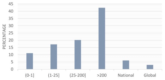
Figure 9.
Distribution of the percentages of studies according to their extension (km2).
We can also analyze the relationships between the extension (km2) of the study and the data sources of the DEM and the reference data (Table 3). First, we analyze the case for the products, then for the reference data and finally, the relations. Table 3 clearly shows that the different sources have extension categories that are more logical to them. For example, LiDAR and Stereophotogrammetry stand out more in smaller range categories and DEMs in broader range categories. The same occurs for topographic maps, but in this case, this source is also present in the global and national categories. Not surprisingly, Ground Surveying, TLS, and GNSS have their largest presences in the smallest extension categories. This situation is logical and has evolved over time (Figure 3). By reducing/increasing the extension, the detail needs are greater/smaller so that preferred data sources (or capture techniques) change in order to offer the needed detail with an appropriate cost and effectivity. The same Table 3 includes the percentage of cases for the case of the reference data. Here, it can be highlighted how GNSS technologies and other topographic surveys have a relevant participation. Due to its past importance, the use of topographic maps appears with relevant values in some categories. For its part, LiDAR appears in some categories in which it competes with GNSS and Ground Surveying techniques. It should be noted that DEM products are the preferred option for the global category and that the use of control infrastructures such as GEDTF is very residual. Finally, a direct comparison of values at each extension and source cross for product sources and reference data clearly indicates different perspectives. We may think that data from one type of data source can be controlled with data from that same type of source; this can happen, but the most logical thing is to go to sources that offer greater accuracy. This is what we believe is evidenced in Table 3 by the observed preference over GNSS techniques and topographic methods, and even LiDAR. In other words, Table 3 confirms that in the production of DEM data and in the evaluation of its positional accuracy, the most suitable data sources are sought for each of the two perspectives.
Table 3.
Cross tabulation between extension (km2) and data sources for products and reference data (% of cases).
4.2. Visual Analysis
Before going into more quantitative aspects, this section will deal with a typology of the quality assessment of DEMs that is quite powerful but also has a certain subjective basis because it is based on the personal experience of the operator. One of the most basic techniques for assessing DEM quality is visual analysis [28,45,46]. Visual analysis is not a quantitative technique, only a qualitative one, but one that quickly reveals the existence of problems in a DEM dataset. The expertise of the analyst is very important but in many occasions also a previous knowledge of the data production flow and the morphology of the terrain helps the visual detection of those sites where there may be problems. In view of Figure 4—Row II, it can be concluded that the vast majority of cases do not contemplate visual evaluation (only 2.91%). Our experience with producers and researchers is that this evaluation process is usually carried out more frequently than indicated in Figure 4—Row II, but that it is not given great importance since it is not usually formalized. We consider that the existence of any kind of document giving clear guidelines on how to carry out this type of analysis would allow greater recognition and confidence in this type of process.
4.3. 1D, 2D + 1D, and 3D Accuracy Assessments
Altimetry (1D) cannot be considered without a planimetric position (2D). It was Koppe (1902) who first indicated the relationship between altimetric and planimetric accuracies, which depends on the slope. This relationship is even present in some standards (e.g., NMAS), which allow some displacement in planimetry to adjust altimetric discrepancies. This dependence of altimetry on planimetry is the reason why traditional planimetric surveying methods have offered better positional accuracies than altimetric ones [1]. Therefore, positional accuracy standards (e.g., NMAS, LMAS, etc.) have established different levels of accuracy for each one of them, and they also propose independent assessments for the planimetric and altimetric accuracies (e.g., NSSDA, etc.). The majority of cases of the corpus are only altimetric accuracy assessments (1D) (Figure 4—Row III). In this 1D case, there are two major options for the statistical analysis, the first one based on the normal distribution model (e.g., NSSDA) and the second on the use of percentiles, as proposed by ASPRS [21] for the case of vegetated areas. We have not found cases where planimetry is used as a way to adjust altimetry (2D + 1D cases). Finally, there few studies (≈4.0%) in which a 3D assessment is carried out [23,47]. 3D analyses are usually based on statistical models other than the ones based on normal distribution.
4.4. Control Elements (Points, Lines, and Surfaces) Used in Accuracy Assessment
The control elements are a subset of the population of interest that are used to carry out the assessment, and they are the reference. As indicated in Section 4.1.3, they must be at least three times more accurate than the data of the product being evaluated. The problem with grid models is that their elements (cells) are not always easily identifiable in the field, and that they do not have an actual existence. To overcome this problem, Ariza-López et.al. [37] proposed a method based on the use of four auxiliary points per control point and the interpolation of the non-identifiable control point. 21.43% of the corpus use the grid model (Figure 10). The GNSS technology (see Section 4.1.3) is mostly used to generate points of high positional accuracy that are used to calculate discrepancies (Equation (1)). Sometimes the use of vertices of an existing geodetic net has been reported [48,49] since these points have an easily-identifiable location. On other occasions, data from spatial platforms such as ICESat [50] or from existing databases such as DTED [51] are used. In Figure 10, we observe that point data is the most frequently used with 67.86%, and this is consistent with what is advanced in Section 4.1.3. Becek (2014) [47] performs the assessment using linear elements (roads, paths, tracks, …), and in this case compares longitudinal profiles obtained from the DEM product against profiles obtained from The Global Elevation Data Testing Facility. This facility is a reference data set of great accuracy with 8500 linear elements. There are many cases in which the assessment is performed using other DEMs [17,42,52,53,54,55,56]. In this situation, it is very common to resample the reference (with the highest accuracy) so that, by means of a spatial superposition of both models with the same spatial resolution, and with the same geographical frame, the comparison is carried out. This does not mean that the comparison is superficial; in short, it is a one-off comparison, since it is the cells of the grid that contrast [57].
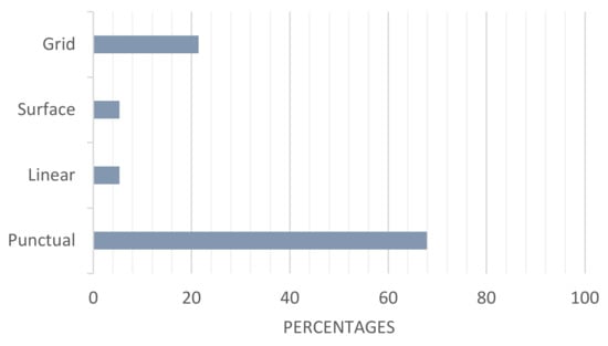
Figure 10.
Percentage distribution of cases according to the geometry of the reference data.
4.5. Calculation of the Discrepancies
The discrepancies presented in Section 2 and formulated in Equation (1) refer to the same position in the DEM and in the reference; however, this calculation can be performed with certain qualifications that must be clarified because, as indicated previously, the problem with grid models is that their elements (cells) are not always easily identifiable in the field, and that they do not have an actual existence.
Kraus et al. (2004) [53] proposed a geometric procedure calculating the discrepancies between a DEM position and the elevation that would correspond to that position, but taking into account the elevations of the closest points and the curvature of the terrain. In this way, there are other studies [47,58,59,60] that also make use of the variability of the elevation where neighbors are taken into account [61]. In other cases, use is made of the analysis of the variability of the elevation in the direction of the rows and columns; they are like crossed topographic profiles [62].
As indicated in the previous subsection, in [37], a method is proposed based on the use of four auxiliary ground survey points per DEM control point, and the interpolation of the non-identifiable control point of the DEM from this set of four points. This set of four auxiliary points must be located on a terrain plane in order to perform a linear interpolation [34].
Despite the fact that interpolation for the contrast between the DEM and the reference data is always necessary, 18.47% of the corpus establishes an analysis of the interpolation method used, generally contrasting between different interpolation methods (Figure 4—Row IV).
4.6. Statistical Model for the Discrepancies
In Section 2, an analysis of the behavior of discrepancies has been performed. In this case, the model based on the normal distribution has been used. This model is explicitly proposed in numerous standards (e.g., EMAS, NSSDA, etc.) and also recognized by various authors (e.g., Oksanen [63]). The vast majority of corpus cases (89.17%) use this model (Figure 4—Row V). The fact that the use of LiDAR technology has increased considerably in recent times means that systematic errors are observed depending on the ground cover, which is why the use of robust statistics is increasingly common. In the first decade of studies analyzed (1990–2000), all of them considered a normal distribution of discrepancies; in the decade from 2001 to 2010, 8.33% considered a non-normal distribution; and this percentage grew to 16.88% in the decade from 2011 to 2019. Thus, in cases where the normal distribution is not considered, robust parameters are used such as the median (Höhle et al. (2009) [64]), percentiles (Maune, [1]), etc. In this way, the problem of the existence of many outliers can be avoided by means of the NMAD (Normalized Median Absolute Deviation), a value that could be compared to the standard deviation in a normal distribution [65]. In [66], a control method is proposed based on the observed discrepancies (non-parametric model), which is controlled by means of various tolerances and a multinomial model for proportions. This method can be considered as an advance in the use of percentiles since a statistical contrast is performed, allowing acceptance or rejection depending on the case. This is not merely descriptive, as reporting a percentile is.
4.7. Sample Size for the Accuracy Assessment
First, it should be noted that this section only focuses on point control elements, since no references have been found for the other types presented in the previous section. Sample size is important because it is related to the representativeness of the sample, but it is not the only element that affects it (e.g., Section 4.8 deals with stratification). It should also be noted that the necessary sample size is highly conditioned by the statistical perspective that is adopted; a perspective of estimation of a quality parameter is not the same as that of quality control.
Sample size is a very relevant aspect to achieving good precision in statistical estimation, as indicated by the theory of statistical sampling [67]. Thinking about a normal distribution of discrepancies, the sample size is directly related to the population size (usually considered infinite), the level of significance and the variance in the population, and indirectly related to the precision of the estimation. In relation to quality control, which is based on hypothesis tests, any sample size ensures type I error (producer risk), and the larger the sample size, the greater the power of the statistical contrast, that is, the ability to detect small deviations from the set point. This is related to type II error (consumer risk). In any case, although there are many documents of the corpus that analyse this aspect, a statistical approach is unusual, an empirical approach is more usual, and many documents do not make clear the statistical approach they take.
Most standards for positional accuracy control recommend a minimum of 20 control points (e.g., NMAS, NSSDA, etc.). FEMA advises 20 control points on each type of vegetation cover that exists in the study area, establishing a classification of five cover types: open terrain, weeds and crops, scrub and bushes, forested and built-up areas. In this way, 100 control points are typically used, 20 for each of the five cover types [34]. STANAG 2215 [35] recommend a minimum of 167 control points in order to estimate a representative positional accuracy index. Zhilin Li [68] indicates that 570 control points are needed in order to obtain a stable value of accuracy in flat areas.
Only recently have positional accuracy standards (e.g., UNE 2016, ASPRS 2014) begun to link the sample size with the size of the area to be controlled. For instance, the last ASPRS standard [22] includes a table with the number of control points according to the number of hectares of the project. As shown in Table 4, the analyzed cases of the corpus show a great diversity in the number of control points used as sample. For instance, Wang et al. (2015) [56] advise the use of 400 control points for an extension of 960 Km2, but this number is 10 times more than the number recommended by the ASPRS [22].
Table 4.
Maximum, minimum, and median values of the number of control data used in the studies according to their extension.
Although not all the extension categories shown in Table 4 have a high and representative number of cases, some interesting conclusions can nevertheless be drawn. As we can see, the maximum and minimum values are quite irregular. However, we observe that the median grows as the extension of the study increases, which indicates a certain coherence. In conclusion, there is no consensus regarding the sample size.
Some of the cases studied present a perspective directly focused on analyzing the influence of the sample size on the evaluation. This can be very important information for achieving an optimal number of control elements and reducing the investment of the assessment. However, an optimal number is somewhat complex due to the number of variables involved. In relation to some positional accuracy standards, there are several theoretical studies (NMAS, EMAS, ASPRS, etc.). In this way, in the corpus there are 5.73% (Figure 4—Row VI) of cases which analyze the accuracy obtained by varying the number of control elements (generally points).
Finally, it should also be noted that there are several studies (e.g., Heritage et al. (2009) [69] and Erdogan (2010) [4]) (Figure 4—Row VII) that offer equations that relate sample size and sampling strategy to the interpolation algorithm and local terrain morphology in order to estimate the DEM accuracy.
4.8. Terrain Segmentation for Accuracy Assessment
As shown in Figure 4—Row VIII, it is not very usual (16.56%) for the terrain to be segmented or divided into zones in which the evaluation of positional accuracy is evaluated and reported. In this way, a single accuracy index is not offered for the entire DEM, rather accuracy indices can be offered for each of the areas under consideration. Reporting by areas is something that has been proposed in some standards ASPRS [21]. The most usual is that the segmentation is a stratification, that is, they are considered zones, connected or not, whose intra-variability is less than that of the population as a whole. This provides a better description of the performance of a DEM in its different sub-areas. ASPRS [22] considers three critical aspects that influence accuracy: different producers and technologies in the data capture, the topographic variation, and the vegetation cover. The criteria for defining these strata can be varied; some common ones are the use of the morphology of the terrain (e.g., flat, undulating, or mountainous) [38,42,70] and the vegetation cover [70,71].
The reasons for the first criterion (morphology) are related to the behavior of the relationship between altimetry and planimetry that has been indicated in Section 4.3. For instance, Zhilin (1991) [68] concluded that regardless of the data capture technology used, the DEM’s accuracy depends on the slope of the terrain, so it may be interesting to change the sampling density spatially in order to collect a sample of each type of terrain according to its slope. In this way, Heritage et al. (2009) [69] and Erdogan (2010) [4] concluded that the accuracy is not a general parameter of the model but has a local behavior depending on its morphology. The tendency of most authors is to think that the most abrupt areas have greater uncertainty than the most undulating or flat areas [72]. This is totally logical, considering that data capture in rough terrain has higher uncertainty than in flat terrain, in all the technologies that can be used in data capture. However, Zhou [73] relates the morphology of the terrain with the uncertainty obtained in derived parameters such as slope and aspect, and concludes that flat areas are the most affected by the uncertainty in slope and aspect; however, in steep areas, the uncertainty of the slope and aspect is quite low. The importance of this criterion is reflected in the high percentage (35.67%) of cases of the corpus (Figure 4—Row IX), which is a very high value in comparison with other possible considerations in DEM accuracy assessments.
The reasons for the second criterion have more to do with the behavior of the data capture technique in relation to the type of vegetation cover. In this way, when LiDAR began to be used as a data capture technology, and from then on, non-normal behavior in the distribution discrepancies in elevations began to be considered in many studies [34,64,74,75,76]. Zandbergen (2011) [74] established that the non-normality of the discrepancies distribution may be due to the outliers, the spatial autocorrelation, and the non-stationary processes that underly the occurrence of vertical discrepancies. The cause is the different accuracy behavior of LiDAR data depending on the type of vegetation cover. In the case of InSAR [77,78], it was observed that the height of the vegetation produces quite high discrepancies, something similar to that observed for the LiDAR technology, but not in such a marked way. The ASPRS standard establishes a fundamental vertical accuracy for open areas (assuming a normal distribution for discrepancies) and a supplementary vertical accuracy for vegetated zones expressed by the 95th percentile. Each vegetation cover should have both a fundamental and supplemental vertical accuracy, whenever possible. As shown in Figure 4—Row X, 15.29% of cases analyze the behavior of accuracy based on ground cover, especially those using LiDAR as data capture technology.
Finally, regarding the spatial and statistical structure of discrepancies in Equation (1), Oksanen [79], using omnidirectional variograms, determines that at distances greater than 300 m, it becomes unstructured. In other studies, the same author [80] concludes that the application of geostatistics can be very problematic because the assumption of stationarity is applied to small areas.
The only reference that relates sample size and strata is ASPRS [22], which recommends a minimum of 20 control points in each of the strata (e.g., representative vegetation cover types within the study area).
In addition to the analysis of the accuracy of the DEM based on the morphology of the terrain and the vegetation cover, as we have previously indicated, there are also 16.56% (Figure 4—Row VIII) of studies that perform an analysis of the variability of the accuracy for the entire study area, without relating this accuracy to a parameter such as slope, aspect, vegetation cover, etc. We believe that these are studies that do not delve into the analysis of the accuracy and the parameters on which it depends.
4.9. Accuracy Assessment by Means of Mathematical Models
A mathematical model is an expression, which can be more or less complex, that relates various variables, some that are considered explanatory, or independent, and others that are explained or dependent. In all cases, the results of the application of a mathematical model are compared with empirical accuracy values. These mathematical models can take into account several independent variables such as the terrain slope, the density of points for the DEM generation, the spatial distribution of these points, the interpolation method, etc. [81] in order to explain the accuracy of a given DEM. As Figure 4—Row VII shows, 10.19% of the cases use a mathematical model to predict the accuracy of the model. Ackermann (1994) [82] establishes the mathematical relationship between the conditions in which a DEM must be developed (depending on the type of terrain, etc.) and its final accuracy. In some more recent studies, mathematical models are proposed in the estimation of the accuracy for DEMs obtained using LiDAR methods in which a normal distribution of discrepancies is not assumed [83]. Kulp et al. (2018) [84] applied artificial neural networks (multilayer Perceptron) to the case of SRTM DEM data. Using a 23-dimensional regression of vertical uncertainty, they can predict the accuracy that a SRTM DEM will give us. However, in general, mathematical models do not give good results when compared with empirical procedures for determining accuracy [62].
Interpolation techniques are mathematical methods that have a great deal of application in the case of DEMs, so there are many documents on these techniques. Kidner (2003) [85] established that the most determining factor in the accuracy of the DEM is the interpolation method. The interpolation methods play an important role from the producer’s side of the DEM as well as for the DEM quality assessment process. Interpolations are necessary to calculate the discrepancies between elevations of the same location of the DEM product and the reference. Some studies focus on the uncertainty propagated from the grid nodes [70,86,87,88] to any point within the same cell [89]. Some studies show the difference between biquadratic, bicubic, and bilinear interpolation algorithms [90]. Other cases are centered on the reduction of the effects due to outliers, e.g., Chen et al. (2016) [91] proposed a robust algorithm based on multi-quadratic interpolation (MQ) methodology on M-estimators (MQ-M). Hu et al. (2009) [92] and Liu et al. (2012) [93] uses the Theory of the Approach to estimate the accuracy of the model considering two components, that coming from propagation of the data and that of the interpolation. Hu et.al. (2009) consider the error of the interpolation as a systematic error. One of the most complete models, which jointly considers the aspects indicated, is the one proposed by Aguilar et al. (2002) [94]. This model established that the accuracy of a DEM is mainly due to three factors: the morphology of the terrain, the point density used for the DEM generation, and the interpolation method used. As shown in Figure 4—Row IV, 18.47% of the cases consider the interpolation method as a determining factor for the accuracy of the DEM.
4.10. Simulation Techniques for Accuracy Assessment
Simulation has been used as a tool for analysing the behaviour of positional accuracy standards (e.g., NMAS, NSSDA, EMAS, ASPRS) and the accuracy of DEMs. Simulation is an easy method to understand because it is based on the reproduction of a known process or system. Simulation can be defined as the construction of a mathematical model to reproduce the characteristics of a phenomenon, system, or process, using a computer in order to obtain information or solve problems [95]. The simulation process on DEMs consists of introducing random disturbances that follow a statistical model [96]. The model is usually the normal distribution, but the spatial component can also be introduced by means of autocorrelations and spatial models in the distribution of the perturbations [56,63,69,75,97,98,99,100,101]. From the pioneering papers of Fisher [102], who applied the simulation on DEM for the determination of hydrographic basins and visual basins, the interest in applying this technique to DEMs was demonstrated. 8.28% (Figure 4—Row XI) of the cases of the corpus use this procedure to later assess the DEM’s accuracy. This method is quite useful since we know a priori the statistical and spatial distribution of the perturbations introduced, something that can give us a lot of data for the validity analysis regarding the quality evaluation procedure used.
4.11. Functional Quality Assessment
We speak about functional quality when we refer to the quality of a DEM applied to a generic use case (for example, the calculation of slopes, orientations, etc.). We speak about “fitness for use” when it comes to a specific use case (for example, the calculation of slopes for a specific civil project). Functional quality refers to how the DEM model works as a model of reality and “fitness for use” to what it offers us for a specific case, and without a doubt, both are related. Fisher [103] was one of the first to raise the need to indicate the suitability of a particular DEM in a specific use or application. Wechsler (2003) [29] pointed out the actual need for the DEM’s user to know accuracy parameters in order to make proper use of them. She believes that it is necessary for the user to know the accuracy as well as the consequences that this may have in subsequent analyses (fitness for use). It is necessary to emphasize that no reference has been found that proposes a guide or standard to evaluate this perspective.
In relation to direct calculations performed with a DEM data, [8] indicates the most usual calculations (e.g., height 75.7%, slope 71.6%, aspect 52.9%, drainage delineation 51.0%, etc.). Accuracy assessment, based on the vertical positional accuracy, is traditionally focused on the first of these calculations. All the previous sections of this paper are focused on this perspective. The accuracy assessment of other parameters (e.g., slope, orientation, drainage network, visibility, etc.) can also be determined by comparison of the derived model with sources of higher accuracy than the assessed one [13,42,102,104,105,106,107,108,109]. Several studies are focused on quality assessments obtained from derived hydraulic models [3,5,15,110,111,112]. Due to the importance of the calculation methods of these parameters, there are also studies that analyze the effect of the computation procedure used to determine these parameters on the final accuracy obtained [96].
In the studies that analyze the quality of DEMs by using derived models (slope, aspect, etc.), very diverse measures are used, for example, in the case of slope models the discrepancies or differences between the slopes obtained in the same location, both in the evaluated DEM and in the reference one. The same happens with orientation. In the case of the hydrographic basins, they are compared in some cases by means of the difference in surface extension of the basin obtained in different DEMs (evaluated and reference).
In relation to the corpus of documents, almost 21% of them determine the accuracy of the DEM by analyzing the behavior in some parameter or derived parameter output from DEM, contrasting with a source of greater accuracy. As shown in Figure 11, most cases use slope, aspect, and curvature as single parameters and drainage networks and watersheds as hydrological outputs to assess the accuracy of the DEM.
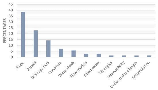
Figure 11.
Distribution of the parameters used in the quality evaluation in different studies.
5. Discussion
This section discusses some relevant aspects related to the major findings presented in the previous section. These findings are related to explicit aspects presented before, but also to evident omissions and detected problems.
One aspect that is explicitly evidenced in the documentation analyzed is the lack of a common vocabulary. We refer to the use of basic but very important terms such as assessment, accuracy, precision, bias, outlier, etc. There are also problems in some documents, and grid models are confused with raster models. This possibly evidences the presence of different overlapping circumstances (e.g., different professional profiles, different application domains, etc.), but also of an inefficient basic standardization regarding DEMs. The geospatial data quality model proposed by international standard ISO 19157 offers a framework, some vocabulary, and even adequate measures, but the use of this standard is simply inexistent. The same is valid for the application of the concepts of GUM and VIM guides. Looking ahead, it is possible that manuals like Maune’s (2019) can help in overcoming these problems.
Directly related to the above is the lack of standardized evaluation methods that are largely assumed by the scientific and technical community. Positional accuracy standards can be applied, but they are not specifically focused on DEM and their degree of application is not very widespread either. DEMs are very important in numerous environmental analyses and engineering projects, but despite this standardized and widely-used procedures have not been achieved. Standard positional accuracy assessment methods (e.g., NMAS, EMAS, ASPRS (2004), NSSDA, ASPRS (2014)) have evolved throughout their existence, and DEM-type data is increasingly present in them (e.g., ASPRS 2014). However, they present a very traditional perspective, the quality of the DEM is controlled by isolated points, and DEMs do not work as isolated points. In the documents analyzed, there are already certain advances towards what is call “fitness for purpose”, which is linked to use cases (see [2] to discover the main use cases of DEMs). We believe that having assessment methods that are closer to the operation and use of DEMs is a key aspect. A relevant aspect is that for the traditional evaluation of the accuracy of the DEM, as proposed by many assessment methods, the planimetric positional component is considered fixed and does not intervene in the calculations of the altimetric accuracy. We believe that this could be overcome with proper 3D evaluation techniques; however, this is unusual.
Linked to the above is the issue of the (non) normality of altimetry discrepancies (di, see Equation (1)). We consider the current situation according to the most advanced proposal, ASPRS, to be problematic. In this case, different methods of evaluating are proposed for normal and non-normal errors. This is logical, but it creates confusion for experts and users and does not offer a common framework. In our opinion, since there is currently a lot of computing power available, parametric (e.g., normal) methods are no longer as relevant, and methods based on multiple tolerances can be applied [66]. These methods can help to resolve in a single common framework the precise control of data mixtures since they are based on tolerable error rates. In any case, assessment methods based on statistical models are the ones mostly being applied so far. However, more sophisticated methods based on artificial intelligence (e.g., artificial neural networks) have already started to appear. It is expected that in the future, these methods will have a higher level of application and that there will be even more local knowledge of how errors occur, something that would allow better accuracy assessments and provide a more functional or “fitness for use” approach.
In the vast majority of studies, quality assessment processes are carried out by interpolating or resampling the reference data. All these processes carried out to match the data from the evaluated DEM product with the reference data introduce an error into the final quantitative result which is never taken into account. We believe that the accuracy assessment process, in addition to being a standardized process, should avoid obtaining data that introduces error into the final result. The Guía para la Evaluación de la Exactitud Posicional de Datos Espaciales [37] proposes a method for choosing points on planes of uniform slope to minimize the error introduced in the interpolation process necessary to obtain the elevation of the point coinciding with the DEM evaluated. Only in this study have we seen a somewhat more specific treatment of this problem.
The totality of the documents analyzed shows that the evaluations of the quality of the DEMs are carried out without informing about the metaquality of the evaluation processes. The metaquality is defined by ISO 19157 as the “information describing the quality of quality data”, and is something almost completely forgotten. Metaquality can be assessed, but it can also be described qualitatively if aspects such as confidence, representativity and homogeneity are adequately reported. However, in many studies, nothing qualitative is reported. We understand that since many of these papers are published in scientific journals, reviewers should be more careful to ensure that the authors better report their evaluation procedures.
Metaquality is related to metadata, so we also have to talk about metadata. In many of the studies analyzed, existing DEMs are used to evaluate another DEM, otherwise the DEM produced is offered as a product to third parties. In both cases, the metadata (of the existing product or of the generated product) are relevant and, within the metadata, the part dedicated to quality. In our study, an exhaustive analysis of these metadata has not been carried out, but the feeling we obtain from what we have analyzed is that the quality part of these metadata either does not exist or is very deficient. Also related to the presentation of results is its visual representation. This is another aspect in which there is great diversity in the documents analyzed. In any case, the spatial representation of the results of the quality assessment is in the minority, and it is also not adequately standardized or channeled by guides from professional or sector organizations.
In the studies that we have analyzed, there are cases that present specific areas and others that focus more on developing methods and new proposals. In the latter case, a great capacity for comparison is lost, as the cases are very diverse and varied. Here it would be highly appropriate for the scientific community to have test bed data sets for testing, so that the researchers would conduct some of their tests using these data sets. Working with these test sets would offer greater comparability of results. This is especially indicated for studies focused on interpolation techniques. Along these lines, Amatulli et al. [113] offer a set of data related to topographic variables for environmental and biodiversity modeling. However, the resolution of these data is not adequate and other variables are required for our case.
To finish the discussion, we will expound two final ideas: (1) the authors believe that a generic quality evaluation process, regardless of technological aspects, has not been sufficiently debugged by the producers. In short, we believe that there should be a standard method of evaluating DEM accuracy that obviates the entire production process and offers (a) valuable parameter(s) of accuracy. (2) An important aspect that we would like to see in the assessment is the use of the fundamental elements of the relief (dividing lines, trough lines, hills, peaks, holes, etc.). These fundamental elements of the relief help to characterize the relief and give greater emphasis to its expression. We believe that they can be key elements in any process of determining the quality of a DEM. The problem with these elements is the ambiguity in their locations.
6. Conclusions
An analysis of how the accuracy assessment of DEMs is evaluated has been presented. This analysis is based on a study of almost 200 references spanning the past three decades. From our point of view, the most relevant conclusion of this paper is that, despite the real importance of the applications of DEMs in numerous fields, and the technological advances for its creation and availability, accuracy assessment remains as an open issue, as there are no specific guidelines (e.g., standards). Of course, there have been notable advances (e.g., better knowledge of the statistical behavior of discrepancies, etc.), but this is not enough, and even less from a functional quality perspective, and even less from a “fitness for use” perspective. For this reason, there are numerous topics in which scientific research and contributions of a more applied nature can be carried out (e.g., normative documents, guides, etc.). Many of these aspects (e.g., vocabulary, standardization, 3D control, meta-quality, data testbeds for comparable tests, etc.) have already been indicated in the discussion section. The quality assessment procedure and documentation of the quality of DEMs is a challenge for the entire geospatial community and requires further attention.
Author Contributions
Conceptualization, F.J.A.-L. and J.L.M.-M.; methodology, F.J.A.-L. and J.L.M.-M.; writing—J.L.M.-M.; writing—review and editing, F.J.A.-L.; supervision, F.J.A.-L.; funding acquisition, F.J.A.-L. All authors have read and agreed to the published version of the manuscript.
Funding
This research was funded by Ministerio de Ciencia, Innovación y Universidades, grant number PID2019-106195RB-I00, which is partially funded by the European Regional Development Fund (ERDF).
Conflicts of Interest
The authors declare no conflict of interest.
References
- Manune, D.F. Digital Elevation Model. Technologies and Applications: The DEM Users Manual, 2nd ed.; American Society for Photogrammetry and Remote Sensing: Bethesda, MD, USA, 2007. [Google Scholar]
- Ariza-López, F.J.; Chicaiza-Mora, E.G.; Mesa-Mingorance, J.L.; Cai, J.; Reinoso-Gordo, J.F. DEMs: An Approach to Users and Uses from the Quality Perspective. Int. J. Spat. Data Infrastruct. Res. 2018, 13, 131–171. [Google Scholar]
- Stolz, A.; Huggel, C. Debris flows in the Swiss National Park: The influence of different flow models and varying DEM grid size on modelling results. Landslides 2008, 5, 311–319. [Google Scholar] [CrossRef]
- Erdogan, S. Modelling the spatial distribution of DEM error with geographically weighted regression: An experimental study. Comput. Geosci. 2010, 36, 34–43. [Google Scholar] [CrossRef]
- Coveney, S.; Fotheringham, A.S.; Charlton, M.; McCarthy, T. Dual-scale validation fo medium-resolution coastal DEM with terrestrial LiDAR DSM and GPS. Comput. Geosci. 2010, 36, 489–499. [Google Scholar] [CrossRef]
- Gonzales de Oliveira, C.; Paradella, W.R.; De Queiroz Da Silva, A. Assessment of radargrammetric DSMs from TerraSAR-X Stripmap images in a mountainous relief area of the Amazon region. ISPRS J. Photogramm. Remote Sens. 2011, 66, 67–72. [Google Scholar] [CrossRef]
- Bühler, Y.; Marty, M.; Ginzler, C. High resolution DEM generation in high-alpine terrain using airborne Remote Sensing techniques. Trans. Gis 2012, 16, 635–647. [Google Scholar] [CrossRef]
- Mesa-Mingorance, J.L.; Chicaiza-Mora, E.G.; Bueaño, X.; Cai, J.; Rodríguez-Pascual, A.F.; Ariza-López, F.J. Analysis of Users and Uses of DEMs in Spain. Int. J. Geo-Inf. 2017, 6, 406. [Google Scholar] [CrossRef]
- He, Y.; Song, Z.; Liu, Z. Updating highway asset inventory using airborne LiDAR. Measurement 2017, 104, 132–141. [Google Scholar] [CrossRef]
- Vanthof, V.; Kelly, R. Water storage estimation in ungauged small reservoirs with the TanDEM-X DEM and multisource satellite observations. Remote Sens. Environ. 2019, 235, 111437. [Google Scholar] [CrossRef]
- Garcia, G.P.B.; Grohmann, C.H. DEM-based geomorphological mapping and landforms characterization of a tropical karst environment in southeastern Brazil. J. S. Am. Earth Sci. 2019, 93, 14–22. [Google Scholar] [CrossRef]
- Sankey, T.T.; McVay, J.; Swetnam, T.L.; McClaran, M.P.; Heilman, P.; Nichols, M. UAV hyperspectral and LiDAR data and their fusion for arid and semi-arid land vegetation monitoring. Remote Sens. Ecol. Conserv. 2018, 4, 20–33. [Google Scholar] [CrossRef]
- Zhang, K.; Gann, D.; Ross, M.; Robertson, Q.; Sarmiento, J.; Santana, S.; Rhome, J.; Fritz, C. Accuracy assessment of ASTER, SRTM, ALOS and TDX DEMs for Hispaniola and implications for mapping vulnerability to coastal flooding. Remote Sens. Environ. 2019, 225, 290–306. [Google Scholar] [CrossRef]
- Zhang, F.; Zhao, P.; Thiyagalingam, J.; Kirubarajan, T. Terrain-influenced incremental watchtower expansion for wildfire detection. Sci. Total Environ. 2019, 654, 164–176. [Google Scholar] [CrossRef]
- Li, L.; Nearing, M.A.; Nichols, M.H.; Polyakov, V.O.; Guertin, D.P.; Cavanaugh, M.L. The effects of DEM interpolation on quantifying soil surface roughness using terrestrial LiDAR. Soil Tillage Res. 2020, 198, 104520. [Google Scholar] [CrossRef]
- Heo, J.; Jung, J.; Kim, B.; Han, S. Digital Elevation Model-Based convolutional neural network modelling for searching of high solar energy regions. Appl. Energy 2020, 262, 114588. [Google Scholar] [CrossRef]
- Bhatta, B.; Shrestha, S.; Shrestha, P.K.; Talchabhadel, R. Evaluation and application of a SWAT model to assess the climate impact on the hydrology of the Himalayan River Basin. Catena 2019, 181, 104082. [Google Scholar] [CrossRef]
- United Nations. The Global Fundamental Geospatial Data Themes; Committee of Experts on Global Geospatial Information Management: New York, NY, USA, 2019; Available online: http://ggim.un.org/meetings/GGIM-committee/9th-Session/documents/Fundamental_Data_Publication.pdf (accessed on 6 July 2020).
- Shen, Z.Y.; Chen, L.; Liao, R.M.; Huang, Q. A comprehensive study of the effect of GIS data on hydrology and non-point source pollution modelling. Agric. Water Manag. 2013, 118, 93–102. [Google Scholar] [CrossRef]
- USBB. United States National Map Accuracy Standards; U.S. Bureau of the Budget: Washington, DC, USA, 1947. [Google Scholar]
- ASPRS. ASPRS Positional Accuracy Standards for Digital Geospatial Data. Photogramm. Eng. Remote Sens. 2015, 81, 1073–1085. [Google Scholar]
- ASPRS. Vertical Accuracy Reporting for LiDAR Data; Martin Flood; ASPRS LiDAR Committee (PAD): Bethesda, MD, USA, 2004. [Google Scholar]
- Seferick, U.G.; Ozendi, M. Comprehensive comparison of VHR 3D spatial data acquired from IKONOS and TerraSAR-X imagery. Adv. Space Res. 2013, 52, 1655–1667. [Google Scholar] [CrossRef]
- DoD. MIL-STD 600001: Mapping Charting and Geodesy Accuracy; U.S. Department of Defense: Washington, DC, USA, 1990. [Google Scholar]
- Florinsky, I.V. Accuracy of local topographic variables derived from digital elevation models. Int. J. Geogr. Inf. Sci. 1998, 12, 47–61. [Google Scholar] [CrossRef]
- ISO. Guide to the Expression of Uncertainty in Measurement; ISO/TEC 98-3 2008; International Standarization Organization: Geneva, Switzerland, 2008. [Google Scholar]
- ISO. 5725-1:1994 Accuracy (Trueness and Precision) of Measurements Methods and Results–Part 1: General Principles and Definitions; TC 69/SC 6; International Standards Organization: Geneva, Switzerland, 1994. [Google Scholar]
- Butler, J.B.; Lane, S.N. Assessment of DEM quality for Characterizing Surface Roughness using Close Range Digital Photogrammetry. Photogramm. Rec. 1998, 16, 271–291. [Google Scholar] [CrossRef]
- Wechsler, S.P. Perceptions of Digital Elevation Model Uncertainty by DEM Users. Urisa J. 2003, 15, 57–64. [Google Scholar]
- MPLMIC. Positional Accuracy Handbook: Using the National Standard for Spatial Data Accuracy to Measure and Report Geographic Data Quality. Minesota Planing Land Management Information Center. 1999. Available online: https://www.mngeo.state.mn.us/committee/standards/positional_accuracy/positional_accuracy_handbook_nssda.pdf (accessed on 9 July 2020).
- ASCE. Map Uses, Scales and Accuracies for Engineering and Associated Purposes; American Society of Civil Engineers, Committee on Cartographic Surveying, Surveying and Mapping Division: New York, NY, USA, 1983. [Google Scholar]
- ASPRS. Accuracy Standards for Large Scales Maps. Photogramm. Eng. Remote Sens. 1989, 56, 1068–1070. [Google Scholar]
- FGDC. FGDC-STD-007: Geospatial Positioning Accuracy Standards, Part 3. National Standard for Spatial Data Accuracy; Federal Geographic Data Committee: Reston, VA, USA, 1998. [Google Scholar]
- FEMA. Guidelines and Specifications for Flood Hazard Mapping Partners. Appendix A: Guidance for Aerial Mapping and Surveying; Federal Emergency Management Agency: Washington, DC, USA, 2003. [Google Scholar]
- STANAG 2215. Evaluation of Land Maps, Aeronautical Charts and Digital Topographic Data; NATO Standardization Agency: Brussels, Belgium, 2010. [Google Scholar]
- AENOR. UNE 148002. Metodología de Evaluación de la Exactitud Posicional de la Información Geográfica; Asociación Española de Normalización y Certificación: Madrid, Spain, 2016. [Google Scholar]
- Ariza-López, F.J.; García-Balboa, J.L.; Rodríguez-Avi, J.; Robledo-Ceballos, J. Guía para la Evaluación de la Exactitud Posicional de Datos Espaciales; Publicación 557, Serie de Documentos Especializados; Instituto Panamericano de Geografía e Historia: Ciudad de Mexico, Mexico, 2019. [Google Scholar]
- Zhilin, L. Variation of the Accuracy of Digital Terrain Models with Sampling Interval. Photogramm. Rec. 1992, 14, 113–128. [Google Scholar]
- Bonin, O.; Rousseaux, F. Digital Terrain Model Computation from Contour Lines: How to derive quality information from artefact analysis. Geoinformatica 2005, 9, 253–268. [Google Scholar] [CrossRef]
- Robinson, G.J. The Accuracy of Digital Elevation Models derived from Digitised Contour Data. Photogramm. Rec. 1994, 14, 805–814. [Google Scholar] [CrossRef]
- Carrara, A.; Bitelli, G.; Carlá, R. Comparison of techniques for generating digital terrain models from contour lines. Int. J. Geogr. Inf. Sci. 1997, 11, 451–473. [Google Scholar] [CrossRef]
- Gao, J. Impact of sampling intervals on the reliability of topographic variables mapped from grid DEMs at a micro-scale. Int. J. Geogr. Inf. Sci. 1998, 12, 875–890. [Google Scholar] [CrossRef]
- Tankagi, M. A study of DEM accuracy according to spatial resolution. In Proceedings of the 17th Asian Conference on Remote Sensing, Colombo, Sri Lanka, 4–8 November 1996. [Google Scholar]
- Mesa-Mingorance, J.L.; Ariza-López, F.J. Evaluación de la Calidad en Modelos Digitales de Elevaciones. Bibliografía Comentada. Cartographic Engineering Research Group, University of Jaén. 2019. Available online: http://coello.ujaen.es/investigacion/web_giic/SubWeb_CartoCalidad/descargas/GIIC_EvaluacionCalidadMDE_Bibliograf%C3%ADaComentada.pdf (accessed on 9 July 2020).
- Bolstad, P.V.; Stowe, T. An Evaluation of DEM Accuracy: Elevation, Slope and Aspect. Photogramm. Eng. Remote Sens. 1994, 60, 1327–1332. [Google Scholar]
- Pipaud, I.; Loibl, D.; Lehmkuhl, F. Evaluation of TanDEM-X elevation data for geomorphological mapping and interpretation in high mountain environments-A case study from SE Tibet, China. Geomorphology 2015, 246, 232–254. [Google Scholar] [CrossRef]
- Becek, K. Assessing Global Digital Elevation Models using the Runway Method: The Advanced Spaceborne Thermal Emission and Reflection Radiometer versus the Shuttle Radar Topography Mission case. IEEE Trans. Geosci. Remote Sens. 2014, 52, 4823–4831. [Google Scholar] [CrossRef]
- Mcneill, S.J.; Belliss, S.E. Assessment of Digital Elevation Model Accuracy using ALOS-PRISM Stereo Imagery. In Proceedings of the 24th International Conference Image and Vision Computing; (IVCNZ 2009), Wellington, New Zealand, 23–25 November 2009. [Google Scholar]
- Liu, X. Accuracy assessment of LiDAR elevation data using survey marks. Surv. Rev. 2011, 43, 80–93. [Google Scholar] [CrossRef]
- Carabajar, C.C.; Harding, D.J.; Suchdeo, V.P. IceSat LiDAR and Global Digial Elevation Models: Applications to DESDYNI. In Proceedings of the International Geoscience and Remote Sensing Symposium, IGARSS, Honolulu, HI, USA, 25–30 July 2010. [Google Scholar]
- Gesch, D.B.; Larson, K.S. Techniques for development of Global 1-Kilometer Digital Elevation Models. In Proceedings of the Pecora Thirteen: Human Interactions with the Environment: Perspective from Space, Sioux Falls, SD, USA, 20–22 August 1997. [Google Scholar]
- Zhang, W.; Wang, W.; Chen, L. Constructing DEM based on InSAR and the Relationship between InSAR DEM’s Precision and Terrain Factors. Energy Procedia 2012, 16, 184–189. [Google Scholar] [CrossRef]
- Mukherjee, S.; Joshi, P.K.; Mukherjee, S.; Ghosh, A.; Garg, R.D.; Mukhopadhyay, A. IU accuracy of open source Digital Elevation Model (DEM). Int. J. Appl. Earth Obs. Geoinf. 2013, 21, 205–217. [Google Scholar] [CrossRef]
- Kinsey-Henderson, A.E.; Wilkinson, S.N. Evaluating Shuttle Radar and interpolated DEMs for slope gradient and soil erosion estimation in low relief terrain. Environ. Model. Softw. 2013, 40, 128–139. [Google Scholar] [CrossRef]
- Avtar, R.; Yunus, A.P.; Kraines, S.; Yamamuro, M. Evaluating of DEM generation based on Interferometric SAR using TanDEM-X data in Tokyo. Phys. Chem. Earth 2015, 83–84, 166–177. [Google Scholar] [CrossRef]
- Wang, B.; Shi, W.; Liu, E. Robust methods for assessing the accuracy of linear interpolated DEM. Int. J. Appl. Earth Obs. Geoinf. 2015, 34, 198–206. [Google Scholar] [CrossRef]
- Isaacson, D.L.; Ripple, W.J. Comparison of 7.5-Minute and 1-Degree Digital Elevation Models. Photogramm. Remote Sens. 1990, 56, 1523–1527. [Google Scholar]
- López, C. Improving the Elevation Accuracy of Digital Elevation Models: A Comparison of Some Error Detection Procedures. Trans. Gis 2000, 4, 43–64. [Google Scholar] [CrossRef]
- López, C. An experiment on the elevation accuracy improvementof photogrammetrically derived DEM. Int. J. Geogr. Inf. Sci. 2002, 16, 361–375. [Google Scholar] [CrossRef]
- Buckley, S.J.; Mitchell, H.L. Integration, validation and point spacing optimisation of digital elevation models. Photogramm. Rec. 2004, 19, 277–295. [Google Scholar] [CrossRef]
- Felicísimo, A.M. Parametric statistical method for error detection in digital elevation models. ISPRS J. Photogramm. Remote Sens. 1994, 49, 29–33. [Google Scholar] [CrossRef]
- López, C. Locating some types of random errors in Digital Terrain Models. Int. J. Geogr. Inf. Sci. 1997, 11, 677–696. [Google Scholar] [CrossRef]
- Oksanen, J.; Sarjakoski, T. Error propagation of DEM-based Surface derivates. Comput. Geosci. 2005, 31, 1015–1027. [Google Scholar] [CrossRef]
- Höhle, J.; Höhle, M. Accuracy assessment of digital elevation models by means of robust statistical methods. ISPRS J. Photogramm. Remote Sens. 2009, 64, 398–406. [Google Scholar] [CrossRef]
- Baltensweiler, A.; Walthert, L.; Ginzler, C.; Sutter, F.; Purves, R.S.; Hanewinkel, M. Terrestrial laser scanning improves digital elevation models and topsoil pH modelling in regions with complex topography and dense vegetation. Environ. Model. Softw. 2017, 95, 13–21. [Google Scholar] [CrossRef]
- Ariza-López, F.J.; Rodríguez-Avi, J.; González-Aguilera, D.; Rodríguez-Gonzálvez, P.A. New Method for Positional Accuracy Control for Non-Normal Errors Applied to Airborne Laser Scanner Data. Appl. Sci. 2019, 9, 3887. [Google Scholar] [CrossRef]
- Ariza-López, F.J.; Rodríguez-Avi, J.; Alba-Fernández, V. A positional quality control test based on proportions. Lect. Notes Geo-Inf. Cartogr. 2018, F3, 349–363. [Google Scholar]
- Zhilin, L. Effects of Check Points on the Reliability of DTM Accuracy Estimates Obtained from Experimental Tests. Photogramm. Eng. Remote Sens. 1991, 57, 1333–1370. [Google Scholar]
- Heritage, G.L.; Milan, D.J.; Large, A.R.G.; Fuller, I.C. Influence of survey strategy and interpolation model on DEM quality. Geomorphology 2009, 112, 334–344. [Google Scholar] [CrossRef]
- Bater, C.W.; Coops, N.C. Evaluating error associated with LiDAR-derived DEM interpolation. Comput. Geosci. 2009, 35, 289–300. [Google Scholar] [CrossRef]
- Goock, M.J.; Chandler, J.H. Accuracy assessment of digital elevation models generated using the Erdas Imagine Orthomax Digital Photogrammetric System. Photogramm. Rec. 1999, 16, 519–531. [Google Scholar] [CrossRef]
- Tang, F.-A.; Strobl, J.; Gong, J.-Y.; Zhao, M.-D.; Chan, Z.-J. Evaluation on the accuracy of digital elevation models. J. Geogr. Sci. 2001, 11, 209–216. [Google Scholar]
- Zhou, Q.; Liu, X.; Sun, Y. Terrain complexity and uncertainties in grid-based digital terrain analysis. Int. J. Geogr. Inf. Sci. 2006, 20, 1137–1147. [Google Scholar] [CrossRef]
- Zandbergen, P.A. Characterizing the error distribution of LiDAR elevation data for North Carolina. Int. J. Remote Sens. 2011, 32, 409–430. [Google Scholar] [CrossRef]
- Chen, C.; Fan, Z.; Ye, T.; Dai, H. A robust estimator for the accuracy assessment of Remote-Sensing derived DEMs. Int. J. Remote Sens. 2012, 33, 2482–2497. [Google Scholar] [CrossRef]
- Baade, J.; Schmullius, C. TanDEM-X IDEM precision and accuracy assessment based on a large assembly of differential GNSS measurements in Kruger National Park, South Africa. ISPRS J. Photogramm. Remote Sens. 2016, 119, 496–508. [Google Scholar] [CrossRef]
- Hodgson, M.E.; Jensen, J.R.; Schmidt, L.; Davis, B. An evaluation of LiDAR and IFSAR-derived digital elevation models in leaf- on conditions with USGS Level 1 and Level 2 DEMs. Remote Sens. Environ. 2003, 84, 295–308. [Google Scholar] [CrossRef]
- Eckert, S.; Kellenberger, T.; Itten, K. Accuracy assessment of automatically derived digital elevation models from Aster data in mountainous terrain. Int. J. Remote Sens. 2005, 26, 1943–1957. [Google Scholar] [CrossRef]
- Oksanen, J. Digital Elevation Model Error in Terrain Analysis; Publications of the Finnish Geodetic Institute; University of Helsinki, University Press: Helsinki, Finland, 2006. [Google Scholar]
- Oksanen, J.; Sarjakoski, T. Uncovering the statistical and spatial characteristics for fine toposcale DEM error. Int. J. Geogr. Inf. Sci. 2006, 20, 345–369. [Google Scholar] [CrossRef]
- Zhilin, L. Mathematical Models of the Accuracy of Digital Terrain Model Surfaces Linearly Constructed from Square Gridded Data. Photogramm. Rec. 1993, 14, 661–674. [Google Scholar]
- Ackermann, F. Digital Elevation Models-techniques and application, quality standards, development. IAPRS J. Photogramm. Remote Sens. 1994, 30, 421–432. [Google Scholar]
- Aguilar, F.J.; Mills, J.P. Accuracy assessment of LiDAR-Derived digital elevation models. Photogramm. Rec. 2008, 23, 148–169. [Google Scholar] [CrossRef]
- Kulp, S.A.; Strauss, B.H. CoastalDEM: A global coastal digital elevation model improved from SRTM using a neural network. Remote Sens. Environ. 2018, 206, 231–239. [Google Scholar] [CrossRef]
- Kidner, D.B. Higher-order interpolation of regular grid digital elevation models. Int. J. Remote Sens. 2003, 24, 2981–2987. [Google Scholar] [CrossRef]
- Kyriakidis, P.C.; Goodchild, M.F. On the prediction error variance of three common spatial interpolation schemes. Int. J. Geogr. Inf. Sci. 2006, 20, 823–855. [Google Scholar] [CrossRef]
- Schwendel, A.C.; Fuller, I.C.; Death, R.G. Assessing DEM interpolation methods for effective representation of upland stream morphology for rapid appraisal of bed stability. River Res. Appl. 2012, 28, 567–584. [Google Scholar] [CrossRef]
- Patel, A.; Katiyar, S.K.; Prasad, V. Performances evaluation of different open source DEM using Differential Global Positioning System (DGPS). Egypt. J. Remote Sens. Space Sci. 2016, 19, 7–16. [Google Scholar] [CrossRef]
- Chen, C.; Yue, T. A method of DEM construction and related error analysis. Comput. Geosci. 2010, 36, 717–725. [Google Scholar] [CrossRef]
- Shi, W.Z.; Li, Q.Q.; Zhu, C.Q. Estimating the propagation error of DEM from higher-order interpolation algorithms. Int. J. Remote Sens. 2005, 26, 3069–3084. [Google Scholar] [CrossRef]
- O´Loughlin, F.E.; Paiva, R.C.D.; Durand, M.; Alsdorf, D.E.; Bates, P.D. A multi-sensor approach towards a global vegetation corrected SRTM DEM product. Remote Sens. Environ. 2016, 182, 49–59. [Google Scholar] [CrossRef]
- Hu, P.; Liu, X.; Hu, H. Accuracy assessment of Digital Elevation Models based on Approximation Theory. Photogramm. Eng. Remote Sens. 2009, 75, 49–56. [Google Scholar] [CrossRef]
- Liu, X.; Hu, P.; Hu, H.; Sherba, J. Approximation Theory Applied to DEM Vertical Accuracy Assessment. Trans. Gis 2012, 16, 397–410. [Google Scholar] [CrossRef]
- Aguilar Torres, F.J.; Aguilar Torres, M.A.; Agüera Vega, F.; Carvajal Ramírez, F.; Sánchez Salmerón, P.L. Efectos de la Morfología del Terreno, Densidad Muestral y Métodos de Interpolación en la Calidad de los Modelos Digitales de Elevaciones. In Proceedings of the XIV Congreso Internacional de Ingeniería Gráfica, INGEGRAF, Santander, Spain, 5–7 June 2002. [Google Scholar]
- Ríos Insua, D.; Ríos Insua, S.; Martín, J. Simulación. Métodos y Aplicaciones; Editorial RA-MA: Madrid, Spain, 1997. [Google Scholar]
- Veregin, H. The Effects of Vertical Error in Digital Elevation Models on the Determination of Flow-path Direction. Cartogr. Geogr. Inf. Syst. 1997, 24, 67–69. [Google Scholar] [CrossRef]
- Delgado-García, J.; Soares, A.; Pérez-García, J.L.; Carvalho, J. Aplicación del método de simulación secuencial directa para la evaluación de la incertidumbre local en Modelos Digitales de Elevaciones. Geofocus Int. Rev. Geogr. Inf. Sci. Technol. 2007, 7, 23–37. [Google Scholar]
- Wise, S. Information entropy as a measure of DEM quality. Comput. Geosci. 2012, 48, 102–110. [Google Scholar] [CrossRef]
- Schmid, K.A.; Hadley, B.; Wijekoon, N. Vetical Accuracy and Use of Topographic LiDAR Data in Coastal Marshes. J. Coast. Res. 2011, 27, 116–132. [Google Scholar] [CrossRef]
- Miller, M.L. Analysis of Viewshed Accuracy with Variable Resolution LiDAR Digital Surface Models and Photogrammetrically-Derived Digital Elevation Models; Virginia Polytechnic and State University: Blacksburg, VA, USA, 2011. [Google Scholar]
- Goulden, T.; Hopkinson, C.; Jamieson, R.; Sterling, S. Sensitivity of DEM, slope, aspectand watershed attributes to LiDAR measurement uncertainty. Remote Sens. Environ. 2016, 179, 23–35. [Google Scholar] [CrossRef]
- Lee, J.; Snyder, P.K.; Fisher, P.F. Modeling the Effect of Data Errors on Feature Extraction from Digital Elevation Models. Photogramm. Eng. Remote Sens. 1992, 58, 1461–1467. [Google Scholar]
- Fisher, P.F.; Tate, N.J. Causes and consequences of error in digital elevation models. Prog. Phys. Geogr. 2006, 30, 467–489. [Google Scholar] [CrossRef]
- Shi, X.; Lynsey, G.; Long, R.; Dekett, R.; Philippe, J.; Burke, T. A comparison of LiDAR-based DEMs and USGS-sourced DEMs in terrain analysis for knowledge-based digital soil mapping. Geoderma 2012, 170, 217–226. [Google Scholar] [CrossRef]
- Yang, P.; Ames, D.P.; Fonseca, A.; Anderson, D.; Shrestha, R.; Glenn, N.F.; Cao, Y. What is the effect of LiDAR-derived DEM resolution on large-scale watershed model results? Environ. Model. Softw. 2014, 58, 48–57. [Google Scholar] [CrossRef]
- Mashimbye, Z.E.; De Clercq, W.P.; Van Niekerk, A. An evaluation of digital elevation models (DEMs) for delineating land components. Geoderma 2014, 213, 312–319. [Google Scholar] [CrossRef]
- Noh, M.J.; Howat, I.M. Automated Coregistration of repeat Digital Elevation Models for Surface elevation change measurement using geometric constraints. IEEE Trans. Geosci. Remote Sens. 2014, 52, 2247–2260. [Google Scholar] [CrossRef]
- Witt, E.C. Evaluation of the U.S. Geological Survey standard elevation products in a two-dimensional hydraulic modelling application for a low relief coastal floodplain. J. Hydrol. 2015, 531, 759–767. [Google Scholar] [CrossRef]
- Leong Tan, M.; Ficklin, D.L.; Dixon, B.; Ibrahim, A.L.; Yusop, Z.; Chaplot, V. Impacts of DEM resolution, source, and resampling technique on SWAT-simulated streamflow. Appl. Geogr. 2015, 63, 357–368. [Google Scholar]
- Chen, C.; Liu, F.; Li, Y.; Yan, C.; Liu, G. A robust interpolation method for constructing digital elevation models from remote sensing data. Geomorphology 2016, 268, 275–287. [Google Scholar] [CrossRef]
- Martínez, C.; Hancock, G.R.; Kalma, J.D.; Wells, T.; Boland, L. An assessment of digital elevation models and their ability to capture geomorphic and hydrologic properties at the catchment scale. Int. J. Remote Sens. 2010, 31, 6239–6257. [Google Scholar] [CrossRef]
- Vaze, J.; Teng, J.; Spencer, G. Impact of DEM accuracy and resolution on topographic indices. Environ. Model. Softw. 2010, 25, 1086–1098. [Google Scholar] [CrossRef]
- Amatulli, G.; Domisch, S.; Tuanmu, M.; Parmentier, B.; Ranipeta, A.; Malczyk, J.; Jetz, W. Data Descriptor: A suite global, cross-scale topographic variables for environmental and biodiversity modelling. Sci. Data 2018, 5, 180040. [Google Scholar] [CrossRef]
© 2020 by the authors. Licensee MDPI, Basel, Switzerland. This article is an open access article distributed under the terms and conditions of the Creative Commons Attribution (CC BY) license (http://creativecommons.org/licenses/by/4.0/).