Reconstruction of Cloud-free Sentinel-2 Image Time-series Using an Extended Spatiotemporal Image Fusion Approach


Abstract
1. Introduction
2. Methods and Process Procedures
2.1. Overview of the Reconstruction Method
- (1)
- Gather the Sentinel-2 image time-series of a study area’s sub-period (t0, t1, t2, …, tn). Without losing generality, assume this period starts at t0 and ends at tn, and the images at t0 and tn are clear-sky ones. Between the two acquisition dates, all other images at dates tk (k = 1, 2, …, n−1) are either partially cloud-covered or fully cloud-covered (with more than 50% cloud coverage). Therefore, all images at tk need to be processed for cloud-free time-series reconstruction. An entire study period can consist of multiple such sub-periods.
- (2)
- Retrieve the time-series MODIS images at the Sentinel-2 image acquisition dates. They are then processed (resampled, re-projected, and geometrically registered with the Sentinel-2 images) for image fusion modelling.
- (3)
- Generate synthetic Sentinel-2 images for all acquisition dates tk (k = 1, 2, …, n−1) from the clear-sky MODIS and Sentinel-2 image pairs at t0 and tn, and MODIS images at tk using PSRFM.
- (4)
- Make a cloud and cloud shadow mask for every cloud contaminated Sentinel-2 image at tk by analyzing the reflectance differences between the observational and synthetic Sentinel-2 images.
- (5)
- Replace the cloudy and cloud shadow pixels of the Sentinel-2 observation images with the corresponding pixels of the synthetic Sentinel-2 images according to the cloud and cloud shadow mask.
- (6)
- Normalize the pixel values of the replacement by calibrating them to the reflectance values of the cloud-free pixels of the same Sentinel-2 observation.
- (7)
- Repeat the steps 3 to 6 until all the images are processed. Then, a cloud-free Sentinel-2 image time-series is reconstructed.
2.2. Brief Description of PSRFM
2.3. Cloud and Cloud Shadow Identification
2.3.1. General Formula
2.3.2. Cloudy Pixel Identification
2.3.3. Cloud Shadow Pixel Identification
2.3.4. Haze Pixel Identification
2.3.5. Normalization of Reconstructed Images
- (1)
- Segment the synthetic Sentinel-2 image into k clusters. The cluster number k can refer to the optimized clusters used for the image blending by PSRFM [24].
- (2)
- Identify, for each cluster, all the cloud-free pixels that are common to the synthetic and observed images and belong to the same cluster, then use the pixel pairs to estimate normalization parameters a and b in Equation (11).
- (3)
- Apply the estimated normalization parameters to map the replacement pixels of the cluster to the observed image.
- (4)
- Repeat steps 2 and 3 for all the clusters.
3. Case Study
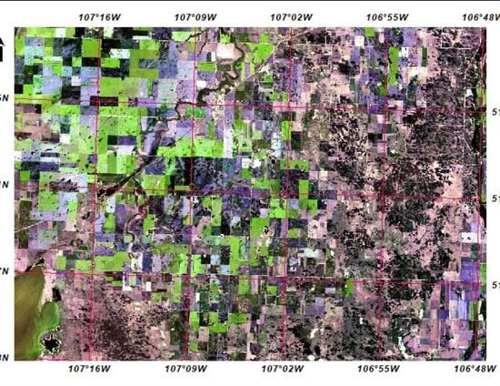
3.1. Study Area
3.2. Image Data
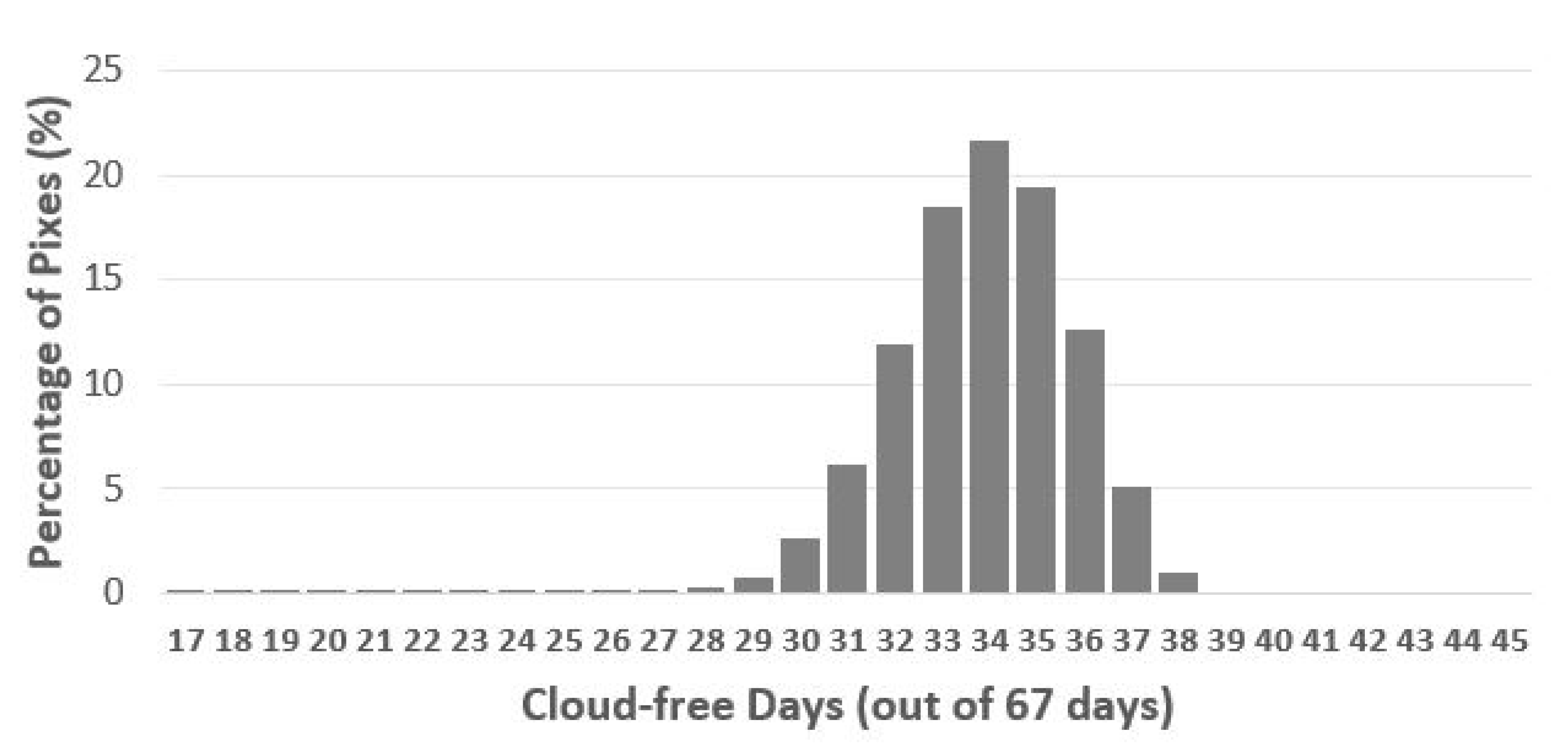
3.2.1. Sentinel-2 MSI Image Time-series
3.2.2. MODIS MCD43A4
3.3. Synthetic Sentinel-2 Image Production by Image Fusion
4. Results and Discussions
4.1. Cloudy, Cloud Shadow, and Haze Pixels Masks
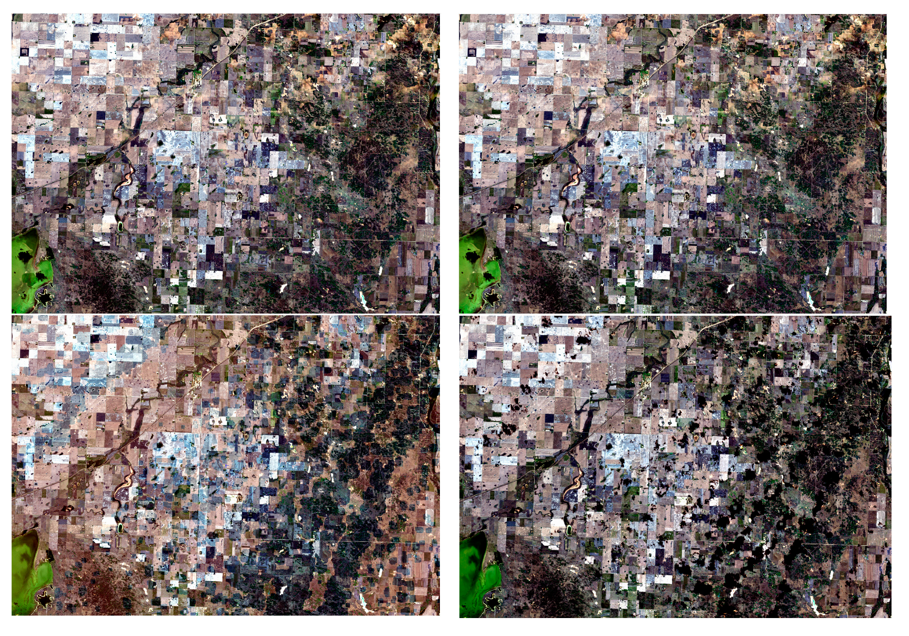
4.2. Reconstruction Results of Cloud-free Sentinel-2 Images
4.3. Normalization Results
4.4. Time-series Normalized Difference Vegetation Index (NDVI)
4.5. Discussions
5. Conclusions
Author Contributions
Funding
Acknowledgments
Conflicts of Interest
References
- Drusch, M.; Bello, U.D.; Carlier, S.; Colin, O.; Fernandez, V.; Gascon, F.; Hoersch, B.; Isola, C.; Laberinti, P.; Martimort, P.; et al. Sentinel-2: ESA’s optical high-resolution mission for GMES operational services. Remote Sens. Environ. 2012, 120, 25–36. [Google Scholar] [CrossRef]
- Djamai, N.; Zhong, D.; Fernandes, F.; Zhou, F. Evaluation of Vegetation Biophysical Variables Time Series Derived from Synthetic Sentinel-2 Images. Remote Sens. 2019, 11, 1547. [Google Scholar] [CrossRef]
- Hunt, M.L.; Blackburn, G.A.; Carrasco, L.; Redhead, J.W.; Rowland, C.S. High resolution wheat yield mapping using Sentinel-2. Remote Sens. Environ. 2019, 233, 111410. [Google Scholar] [CrossRef]
- Granska, E.; Hostert, P.; Pflugmacher, D.; Ostapowicz, K. Forest Stand Species Mapping Using the Sentinel-2 Time Series. Remote Sens. 2019, 11, 1197. [Google Scholar] [CrossRef]
- Rapinel, S.; Mony, C.; Lecoq, L.; Clément, B.; Thomas, A.; Hubert-Moy, L. Evaluation of sentinel-2 time-series for mapping floodplain grassland plant communities. Remote Sens. Environ. 2019, 223, 115–129. [Google Scholar] [CrossRef]
- Fauvel, M.; Lopes, M.; Dubo, T.; Rivers-Moore, J.; Frison, P.; Gross, N.; Ouin, A. Prediction of plant diversity in grasslands using Sentinel-1 and -2 satellite image time series. Remote Sens. Environ. 2020, 237, 111536. [Google Scholar] [CrossRef]
- Zhou, F.; Zhang, A. Methodology for estimating availability of cloud-free image composites: A case study for southern Canada. Int. J. Appl. Earth Obs. Geoinf. 2013, 21, 17–31. [Google Scholar] [CrossRef]
- Wang, Q.; Atkinson, P.M. Spatio-temporal fusion for daily Sentinel-2 images. Remote Sens. Environ. 2018, 204, 31–42. [Google Scholar] [CrossRef]
- Melgani, F. Contextual reconstruction of cloud-contaminated multitemporal multispectral images. IEEE Trans. Geosci. Remote Sens. 2006, 44, 442–455. [Google Scholar] [CrossRef]
- Meng, Q.; Borders, B.E.; Cieszewski, C.J.; Madden, M. Closest Spectral Fit for Removing Clouds and Cloud Shadows. Photogramm. Eng. Remote Sens. 2009, 75, 569–576. [Google Scholar] [CrossRef]
- Chen, J.; Zhu, X.; Vogelmann, J.E.; Gao, F.; Jin, S. A simple and effective method for filling gaps in Landsat ETM+ SLC-off images. Remote Sens. Environ. 2011, 115, 1053–1064. [Google Scholar] [CrossRef]
- Zhu, X.; Liu, D.; Chen, J. A new geostatistical approach for filling gaps in Landsat ETM+ SLC-off images. Remote Sens. Environ. 2012, 124, 49–60. [Google Scholar] [CrossRef]
- Cheng, Q.; Shen, H.; Zhang, L.; Yuan, Q.; Zeng, C. Cloud removal for remotely sensed images by similar pixel replacement guided with a spatio-temporal MRF model. ISPRS J. Photogramm. Remote Sens. 2014, 92, 54–68. [Google Scholar] [CrossRef]
- Zhu, Z.; Woodcock, C.E.; Holden, C.; Yang, Z. Generating synthetic Landsat images based on all available Landsat data: Predicting Landsat surface reflectance at any given time. Remote Sens. Environ. 2015, 162, 67–83. [Google Scholar] [CrossRef]
- Zhu, X.; Helmer, E.H.; Chen, J.; Liu, D. An Automatic System for Reconstructing High-Quality Seasonal Landsat Time-Series. Chapter 2 (Pages 25–42). In Remote Sensing: Time Series Image Processing; Taylor and Francis Series in Imaging Science; Weng, O., Ed.; CRC Press: Boca Raton, FL, USA, 2018; 263p. [Google Scholar]
- Wu, W.; Ge, L.; Luo, J.; Huan, R.; Yang, Y. A Spectral–Temporal Patch-Based Missing Area Reconstruction for Time-Series Images. Remote Sens. 2018, 10, 1560. [Google Scholar] [CrossRef]
- Pouliot, D.; Latifovic, R. Reconstruction of Landsat time series in the presence of irregular and sparse observations: Development and assessment in north-eastern Alberta, Canada. Remote Sens. Environ. 2018, 204, 979–996. [Google Scholar] [CrossRef]
- Gao, F.; Masek, J.; Schwaller, M.; Hall, F. On the blending of the Landsat and MODIS surface reflectance: Predicting daily Landsat surface reflectance. IEEE Trans. Geosci. Remote Sens. 2006, 44, 2207–2218. [Google Scholar]
- Zhu, X.; Chen, J.; Gao, F.; Chen, X.; Masek, J.G. An enhanced spatial and temporal adaptive reflectance fusion model for complex heterogeneous regions. Remote Sens. Environ. 2010, 114, 2610–2623. [Google Scholar] [CrossRef]
- Hilker, T.; Wulder, M.A.; Coops, N.C.; Linke, J.; McDermid, G.; Masek, J.G.; Gao, F.; White, J.C. A new data fusion model for high spatial- and temporal-resolution mapping of forest disturbance based on Landsat and MODIS. Remote Sens. Environ. 2009, 113, 1613–1627. [Google Scholar] [CrossRef]
- Zhukov, B.; Oertel, D.; Lanzl, F.; Reinhackel, G. Unmixing-based multisensor multiresolution image fusion. IEEE Trans. Geosci. Remote Sens. 1999, 37, 1212–1226. [Google Scholar] [CrossRef]
- Huang, B.; Zhang, H. Spatio-temporal reflectance fusion via unmixing: Accounting for both phenological and land-cover changes. Int. J. Remote Sens. 2014, 35, 6213–6233. [Google Scholar] [CrossRef]
- Zhu, X.; Helmer, E.H.; Gao, F.; Liu, D.; Chen, J.; Lefsky, M.A. A flexible spatiotemporal method for fusing satellite images with different resolutions. Remote Sens. Environ. 2016, 172, 165–177. [Google Scholar] [CrossRef]
- Zhong, D.; Zhou, F. A prediction smooth method for blending Landsat and moderate resolution imagine spectroradiometer images. Remote Sens. 2018, 10, 1371. [Google Scholar] [CrossRef]
- Zhou, F.; Zhong, D. Kalman Filter method for generating time-series synthetic Landsat images and their uncertainty from Landsat and MODIS observation. Remote Sens. Environ. 2020, 239, 111628. [Google Scholar] [CrossRef]
- Zhong, D.; Zhou, F. Improvement of Clustering Method for Modelling Abrupt Land Surface Changes in Satellite Image Fusions. Remote Sens. 2019, 11, 1759. [Google Scholar] [CrossRef]
- Zhai, H.; Zhang, H.; Zhang, L.; Li, P. Cloud/shadow detection based on spectral indices for multi/hyperspectral optical remote sensing imagery. ISPRS J. Photogramm. Remote Sens. 2018, 144, 235–253. [Google Scholar] [CrossRef]
- Qiu, S.; Zhu, Z.; He, B. Fmask 4.0: Improved cloud and cloud shadow detection in Landsats 4–8 and Sentinel-2 imagery. Remote Sens. Environ. 2019, 231, 111205. [Google Scholar] [CrossRef]
- Schaaf, C.B.; Gao, F.; Strahler, A.H.; Lucht, W.; Li, X.; Tsang, T.; Strugnell, N.C.; Zhang, X.; Jin, Y.; Muller, J.P.; et al. First operational BRDF, albedo nadir reflectance products from MODIS. Remote Sens. Environ. 2002, 83, 135–148. [Google Scholar] [CrossRef]
- Schaaf, C.; Wang, Z. MCD43A4 MODIS/Terra+Aqua BRDF/Albedo Nadir BRDF Adjusted Ref Daily L3 Global-500m V006 [Data Set]. NASA EOSDIS Land Processes DAAC. 2015. Available online: https://doi.org/10.5067/MODIS/MCD43A4.006 (accessed on 11 August 2020).


| Band Name | Sentinel-2A * MSI | MODIS (MCD43A4) | ||||
|---|---|---|---|---|---|---|
| Band ID | Bandwidth (nm) | Spatial Resolution (m) | Band ID | Bandwidth (nm) | Spatial Resolution (m) | |
| Blue | b2 | 439–533 | 10 | b3 | 459–479 | 500 |
| Green | b3 | 538–583 | 10 | b4 | 545–565 | 500 |
| Red | b4 | 646–684 | 10 | b1 | 620–670 | 500 |
| Near-infrared (NIR) | b8A | 837–881 | 20 | b2 | 841–876 | 500 |
| Shortwave infrared (SWR1) | b11 | 1539–1682 | 20 | b6 | 1628–1652 | 500 |
| Shortwave infrared (SWR2) | b12 | 2078–2320 | 20 | b7 | 2105–2155 | 500 |
© 2020 by the authors. Licensee MDPI, Basel, Switzerland. This article is an open access article distributed under the terms and conditions of the Creative Commons Attribution (CC BY) license (http://creativecommons.org/licenses/by/4.0/).
Share and Cite
Zhou, F.; Zhong, D.; Peiman, R. Reconstruction of Cloud-free Sentinel-2 Image Time-series Using an Extended Spatiotemporal Image Fusion Approach. Remote Sens. 2020, 12, 2595. https://doi.org/10.3390/rs12162595
Zhou F, Zhong D, Peiman R. Reconstruction of Cloud-free Sentinel-2 Image Time-series Using an Extended Spatiotemporal Image Fusion Approach. Remote Sensing. 2020; 12(16):2595. https://doi.org/10.3390/rs12162595
Chicago/Turabian StyleZhou, Fuqun, Detang Zhong, and Rihana Peiman. 2020. "Reconstruction of Cloud-free Sentinel-2 Image Time-series Using an Extended Spatiotemporal Image Fusion Approach" Remote Sensing 12, no. 16: 2595. https://doi.org/10.3390/rs12162595
APA StyleZhou, F., Zhong, D., & Peiman, R. (2020). Reconstruction of Cloud-free Sentinel-2 Image Time-series Using an Extended Spatiotemporal Image Fusion Approach. Remote Sensing, 12(16), 2595. https://doi.org/10.3390/rs12162595