Article

Ensemble Modelling of Skipjack Tuna (Katsuwonus pelamis) Habitats in the Western North Pacific Using Satellite Remotely Sensed Data; a Comparative Analysis Using Machine-Learning Models

1
Regional Center for Mapping of Resources for Development, Nairobi 00618, Kenya
2
Arctic Research Center, Hokkaido University, Sapporo 001-0021, Japan
*
Author to whom correspondence should be addressed.
Remote Sens. 2020, 12(16), 2591; https://doi.org/10.3390/rs12162591
Submission received: 6 July 2020 / Revised: 5 August 2020 / Accepted: 6 August 2020 / Published: 12 August 2020
(This article belongs to the Special Issue Remote Sensing for Fisheries and Aquaculture)

Abstract

:
To examine skipjack tuna’s habitat utilization in the western North Pacific (WNP) we used an ensemble modelling approach, which applied a fisher- derived presence-only dataset and three satellite remote-sensing predictor variables. The skipjack tuna data were compiled from daily point fishing data into monthly composites and re-gridded into a quarter degree resolution to match the environmental predictor variables, the sea surface temperature (SST), sea surface chlorophyll-a (SSC) and sea surface height anomalies (SSHA), which were also processed at quarter degree spatial resolution. Using the sdm package operated in RStudio software, we constructed habitat models over a 9-month period, from March to November 2004, using 17 algorithms, with a 70:30 split of training and test data, with bootstrapping and 10 runs as parameter settings for our models. Model performance evaluation was conducted using the area under the curve (AUC) of the receiver operating characteristic (ROC), the point biserial correlation coefficient (COR), the true skill statistic (TSS) and Cohen’s kappa (k) metrics. We analyzed the response curves for each predictor variable per algorithm, the variable importance information and the ROC plots. Ensemble predictions of habitats were weighted with the TSS metric. Model performance varied across various algorithms, with the Support Vector Machines (SVM), Boosted Regression Trees (BRT), Random Forests (RF), Multivariate Adaptive Regression Splines (MARS), Generalized Additive Models (GAM), Classification and Regression Trees (CART), Multi-Layer Perceptron (MLP), Recursive Partitioning and Regression Trees (RPART), and Maximum Entropy (MAXENT), showing consistently high performance than other algorithms, while the Flexible Discriminant Analysis (FDA), Mixture Discriminant Analysis (MDA), Bioclim (BIOC), Domain (DOM), Maxlike (MAXL), Mahalanobis Distance (MAHA) and Radial Basis Function (RBF) had lower performance. We found inter-algorithm variations in predictor variable responses. We conclude that the multi-algorithm modelling approach enabled us to assess the variability in algorithm performance, hence a data driven basis for building the ensemble model. Given the inter-algorithm variations observed, the ensemble prediction maps indicated a better habitat utilization map of skipjack tuna than would have been achieved by a single algorithm.

Graphical Abstract

1. Introduction

Species distribution modelling is based on the ecological niche concept, which is considered as the volume in the environmental space that permits positive growth of a species [1,2]. The ecological niche concept provides a theoretical basis upon which the fundamental relationships between a species distribution and habitat are established [3]. While the concept is thought to address four main facets: niche characteristics, niche interactions, community-wide processes and niche evolution, species distribution modelling and habitat suitability models mainly contribute to the understanding of niche characteristics [3]. Habitat suitability modeling is widely applied to model and predict habitats of highly migratory pelagic species [4,5], fishery hotspots [6,7] as well as habitat overlaps [8]. In many of these studies, the relationship between the species presence (occurrence) and the environment is established using single habitat suitability modeling algorithms. The scientific knowledge made available from such work has broadened our understanding of the utilization of the marine environment by pelagic species, and contributes significantly to management decisions around resource harvesting, conservation, and the effects of climate change.
Recent advances in the use of ensemble models has demonstrated that they have the capacity to improve the accuracy and predictive power of individual models, addressing model-based uncertainty [9], as well as provide a modelling framework where inherent limitations of constituent algorithms can be observed. A recent review by [9] on the best practices for working with marine species distribution models recommended the implementation of multi-algorithm ensemble techniques that account for the degree of similarity and/or variance between model outputs. The authors also recommended the assessment of model accuracy based on multiple validation scores, as well as extrapolation of model outputs in space or time. By employing multi-algorithm approaches, it is possible to compare the outputs using different algorithms and, therefore, derive more robust results. The increasing adoption of ensemble modelling techniques is consistent with developments in computing technologies through hardware, software and algorithm innovations, which has also given rise to several ensemble species distribution modelling software packages. The Biomod [10], OpenModellor [11], ModEco [12], dismo [13], mopa [14], sdm [15] and Aquamaps [16] packages are among the widely used software packages for ensemble modelling. Each of these softwares have their strengths and limitations which are also dependent on user experience and preferences, hardware and software specifications, number of algorithms implemented, support and maintenance of the packages among other factors. Nevertheless, there are obvious advantages associated with using a software package that calls a number of algorithms in one platform, among them, the ability to fit models using a suite of algorithms concurrently from the same dataset, undertake model performance evaluations using a suite of performance metrics, model selection and predictions on the same platform. Furthermore, a multi-algorithm platform minimizes input data manipulations as a result of software architecture variations, and eliminates platform specific disparities in data file formats and computational adjustments.
For marine applications, the importance of multi-algorithm models in pelagic species habitat predictions has been shown in conservation planning [17], assessing the impacts of climate change [18], invasive species distributions [19], exploring the functional relationships between the marine organisms and their environment [20,21], and fishery forecasting [7,9]. The application of multi-algorithm and ensemble models for fishery hotspot studies in squids [22], tunas [23], whale sharks [24], and marine biodiversity [18] has shown that ensemble models provide more robust habitat information. The performances of the individual algorithms contributing to the ensembles can be evaluated, which helps in optimization of the ensemble model [25], in addition to the ability to vary individual algorithm parameterization settings. Some of the important factors shaping recent applications of ensemble modeling in marine habitat studies include: (i) increased number of user friendly open-source modelling platforms which diversifies choice; (ii) implementation of multiple algorithms in open-source packages which were previously only operable as single algorithm packages; (iii) implementation of comprehensive functionalities for model performance evaluation using a wide range of metrics; (iv) inclusion of functions to create ensemble predictions; and (v) availability of a variety of geo-referenced marine species distribution datasets as response variables, satellite datasets for use as input predictor variables of current conditions, and predicted climate datasets which represent future conditions [26,27]. From this background, we found it feasible to apply a multi-algorithm modelling approach to derive skipjack tuna habitats in the western North Pacific, where to the best of our knowledge such an approach has not been employed for skipjack tuna with the number of algorithms we have used. Our choice of the sdm package was informed by its ability to execute a suite of 17 algorithms using RStudio, and allow for substantial flexibility in evaluation of model performance, predictions and generation of ensemble models [9,15].
The skipjack tuna (Katsuwonus pelamis) fishery in the western North Pacific is closely associated with the seasonal migration of the fish northwards from spring to summer, and southwards at the onset of winter, which is closely linked to feeding [28,29]. The fish track highly productive areas around oceanographic features observable from sea surface temperature (SST) and ocean color gradients, eddies and warm streamers [8,30,31]. They inhabit the upper mixed layer [32,33], and are opportunistic predators which feed voraciously on pelagic fishes, squids, a variety of crustaceans and young skipjacks [34,35]. They are known to migrate over large areas in search of high concentrations of forage [32]. Consequently, these bio-physical oceanographic signals with strong trophic linkages are important indicators of skipjack tuna aggregation sites. The signals are easily monitored with satellite observations and are, therefore, very useful for modeling skipjack tuna habitat formations through correlative or machine learning techniques. Various studies have provided detailed information on skipjack tuna habitat, both from surface [5,8,36] and sub-surface variables [37,38]. The role of temperature, chlorophyll-a concentration and currents in skipjack tuna habitat characterization is well known from several studies [21,29]. For instance, a lower limit SST at 18 °C, surface chlorophyll-a at 0.2–0.3mg/L and warm core eddies in the western North Pacific have been shown to indicate frontal oceanographic features that define skipjack tuna habitat [8,30,36].
Much of the work done on skipjack tuna habitat in the western North Pacific either using surface satellite data or sub-surface data relies heavily on single algorithm computations to relate tuna occurrence to their environment [5,29,30,36,37,39]. These studies are fundamental in elucidating skipjack tuna’s habitat utilization, and can be enriched by exploring algorithms which have received little attention in this field. While multi-algorithm ensemble habitat predictions have been tried for other species in the North Pacific [22], we did not find work that has explored skipjack tuna habitat utilization in the western North Pacific using multi-algorithm species distribution models, hence our work seeks to enhance previous studies in this area [5,8,36]. Our specific objectives were: (i) to model skipjack tuna habitats in the western North Pacific using a suite of 17 presence-only species distribution algorithms and remotely sensed information; (ii) compare the performances of these algorithms using model performance metrics; and (iii) generate ensemble predictions of habitat suitability maps using the sdm package.

2. Materials and Methods
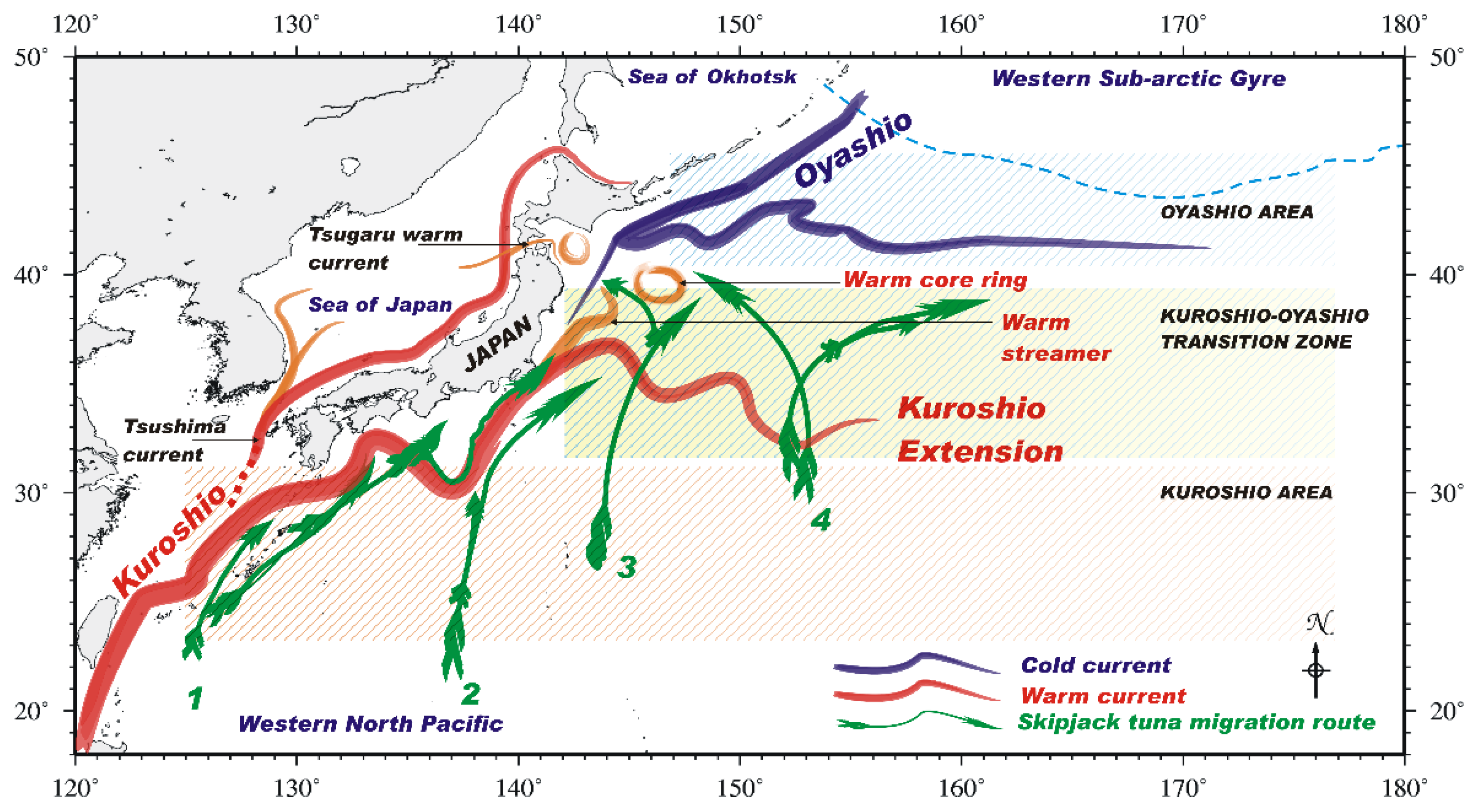
2.1. Study Area

The skipjack tuna caught in the western North Pacific (WNP) off Japan (18–50° N and 125–180° E) arrive in the area via the Nansei Islands and the Pacific Coast of Japan [40]. The oceanographic features in this area influence the migration routes (Figure 1) of the fish as they migrate north [29,41]. The Kuroshio Current, which assumes three major paths south of Japan, is of critical importance to the skipjack’s migration because it transports warm oligotrophic waters, forming pathways for migration, hence influencing formation of pelagic fisheries [42]. The behavior of the Kuroshio Extension, warm streamers and warm core rings (WCR) in the productive Kuroshio Oyashio Transition Zone (KOTZ) is an important feeding and migratory area for skipjacks, which also influences fishing ground formation [30,31]. Further north, towards the northern limit of skipjack tuna migration, the cold Oyashio Current waters flow southward [43], transporting low temperature, low salinity and nutrient rich waters to the sub-tropical gyre [44], and forming two southward tongue-shaped intrusions off Honshu, known as the First and Second Oyashio Intrusions [42,45]. These cold Oyashio waters and the Oyashio Front [46] inhibit skipjack tuna’s northern migration because they avoid waters whose SSTs are below 18 °C [29]. The Oyashio meanders are separated by a WCR originating from the northward movement of the ring produced by the Kuroshio [47], and the frontal zones between the WCR and the meanders are key foraging areas [8]. The behavior of the major currents also influences the lower trophic level dynamics through the distribution and circulation of nutrients, hence the density of phytoplankton and zooplankton populations in the WNP [42]. The high densities of phytoplankton in high nutrient waters subsequently support large populations of various zooplankton species, which are fed upon by smaller nekton [43,46,48]. This creates a downstream trophic chain where skipjack tuna and other pelagic predators exploit such areas of high productivity to forage on the small organisms (squids, crustaceans, and fishes) [7,29,31,32]. Consequently, fishers of skipjack tuna in the WNP often track oceanographic features such as thermal and ocean color fronts, upwelling zones, and edges of large eddies [5,49], to locate areas with dense aggregations of skipjack tuna.

2.2. Fishery Data

Fishery data are often used as indicators of a species presence. We obtained daily skipjack tuna catch data from the Ibaraki Prefecture Fisheries Research Station, covering March to November 2004, the period when the skipjack tuna fishery is active in this area. These data were recorded from pole and line vessels fishing for skipjack tuna in the study area, which usually record their fishing locations and catches. The data were digitized, compiled into monthly composites and converted into 0.25° resolution grids [50] in cells where catches were positive. Re-gridding the data was necessary to ensure that the fishery data matched the resolution of the environment grids. Matching the gridded presence data to predictor variables for a corresponding time period provides a record of the environmental conditions prevailing at the location where the fish were caught.

2.3. Environmental Data

A monthly predictor variable database was compiled consisting of SST, sea surface chlorophyll-a (SSC), and sea surface height anomalies (SSHA). Given their importance as environmental predictors of skipjack tuna habitat [28,41], the three variables are widely used in modelling studies. Skipjack tuna have a wide tolerance range for ambient temperature, hence SST data are an important indicator of their distribution patterns [32,41]. The SSC data provide information on ocean productivity [51], and are important for detecting fronts and eddies that are not always evident in SST maps [52,53]. The elevated productivity around these features attracts large schools of tuna, which aggregate around them to feed on lower trophic level organisms [6,31]. The SSHA data are an indicator of ocean dynamic topography, which provides information on movement of water masses, and by extension the flow of heat and nutrients, which subsequently influence productivity [54]. We downloaded daily resolved optimally interpolated SST global data from the National Oceanic and Atmospheric Administration’s (NOAA) National Climatic Data Center (NCDC) (Table 1), for the year 2004. The optimally interpolated data from the Advanced Very High Resolution Radiometer (AVHRR) and Advanced Microwave Scanning Radiometer on the Earth Observing System (AMSR-E) provided better coverage of the fishing locations because the effect of missing data due to clouds is eliminated. Monthly Aqua-MODIS (Moderate Resolution Imaging Spectroradiometer) ~4 km standard mapped images of SSC for 2004 were downloaded from the National Aeronautics and Space Administration (NASA) Ocean Color data portal (Table 1). The monthly averaged SSHA data were downloaded from the BloomWatch 180 portal (Table 1). Data processing (monthly averaging and sub-setting) and mapping was undertaken in the SeaWiFS (Sea-viewing Wide Field-of-view Sensor) Data Analysis System (SeaDAS) [55] version 5.3 and the Generic Mapping Tools (GMT) version 6.0.0 [56].

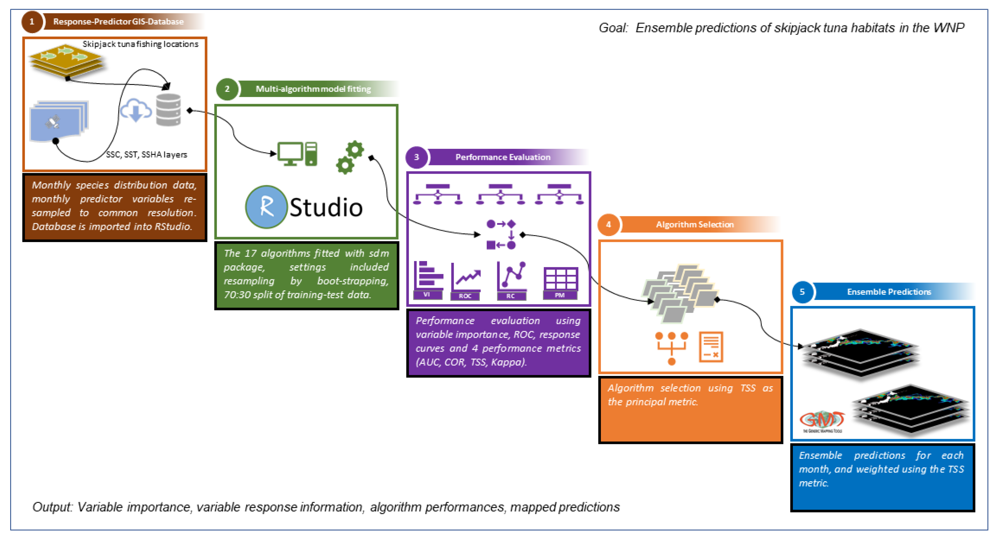
2.4. Habitat Modeling Using sdm Package

The sdm package is based on a framework that uses presence-only data to compute habitat suitability indices (HSI), where the values closer to or equal to 1 represent the high potential habitat areas, and those close to zero represent poor habitat areas. The package comprises a suite of 17 algorithms, whose operation in RStudio provides an ideal platform with sufficient flexibility to adjust for algorithm selection, the associated parameter settings and generation of ensembles. We constructed 9 monthly habitat models in RStudio (version 3.6.1) using the 17 algorithms implemented in the sdm package [15]. We created a script in RStudio which loads all the necessary R packages as described by [15], ingests the fishery data and environmental variable ASCII grids, and subsequently calls the respective algorithms for model fitting, performance evaluation, algorithm selection and ensemble predictions. The skipjack tuna presence data were used as the presence variable and the SST, SSC and SSHA as predictor environmental variables. We applied a 70:30 split for training and test data respectively [57,58], with replication by bootstrapping, for 10 runs. In the bootstrapping technique, sampling with replacement is repeated, each time a sample with equal size as the original data is drawn and used for training data. The observations that are not selected are used for the evaluation at each run [15]. We used variable importance plots to assess the contribution of each predictor variable to model fit, and the response curves to show the relationship between the probability of occurrence of skipjack tuna and each of the predictor variables. Table 2 provides a summary of the 17 algorithms used and their dependent packages in R.

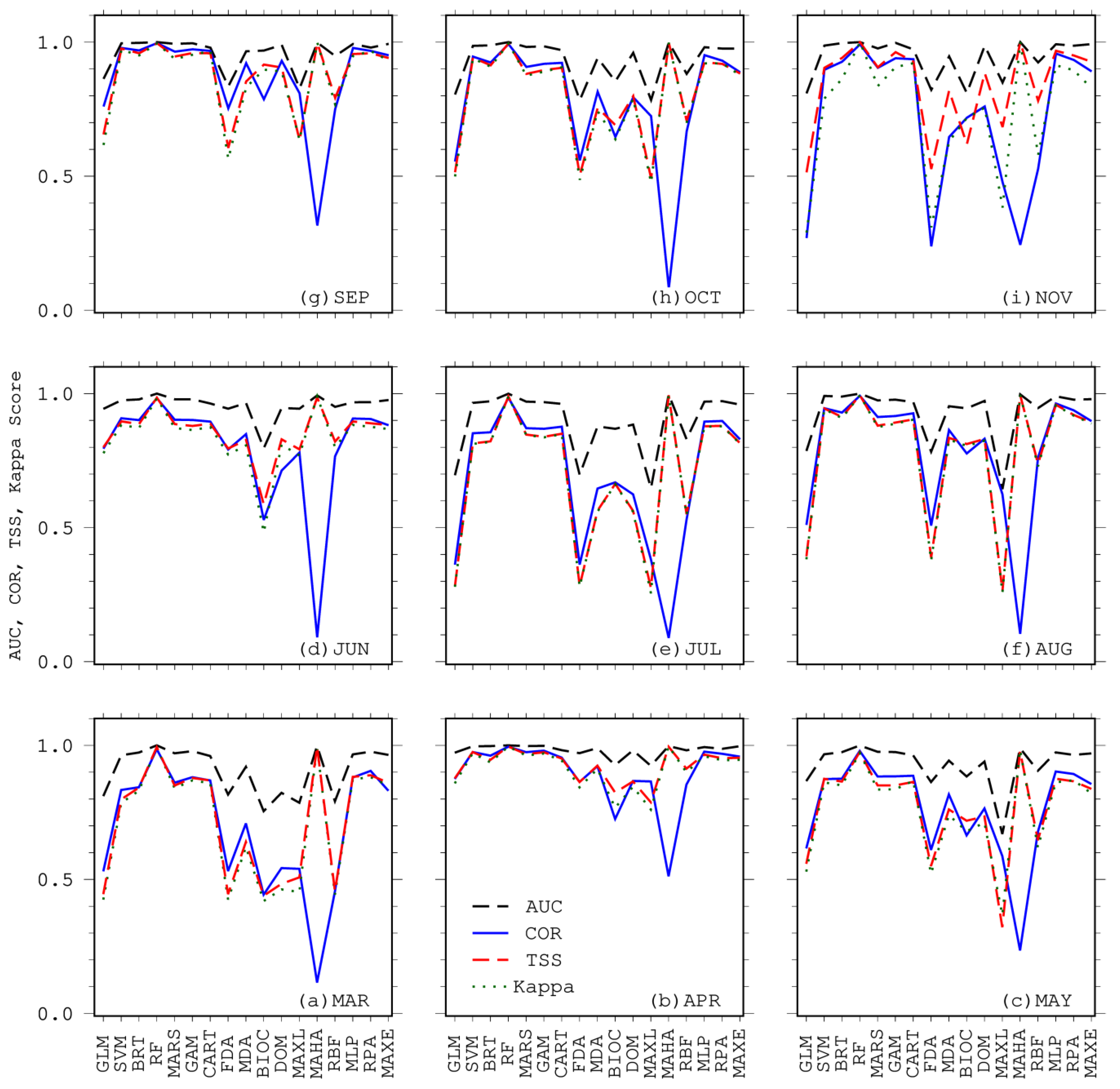
2.5. Evaluation of Model Performance

We evaluated the performance of our models using a multi-metric approach consisting of the area under the curve (AUC) of the receiver operating characteristic (ROC), the point biserial correlation coefficient (COR), the true skill statistic (TSS) and Cohen’s kappa (k) metrics, which is an approach that has been applied in other studies [22,59]. The AUC metric measures the ability of a model to discriminate between sites where a species is present, versus those where it is absent, which provides an indication of the usefulness of the models for prioritizing areas in terms of their relative importance as habitat for the particular species [60]. The AUC ranges from 0 to 1, where a score of 1 indicates perfect discrimination, a score of 0.5 implies predictive discrimination that is no better than a random guess, and values <0.5 indicate performance worse than random [60,61]. The COR is the correlation between the observation in the presence-absence (pseudo-absences) dataset (a dichotomous variable) and the prediction, and is calculated as a Pearson correlation coefficient [61]. It is similar to AUC, but also accounts for how far the prediction varies from the observation, which gives further insight into the distribution of the predictions [61]. The TSS, calculated as sensitivity plus specificity less one, is an improvement of the k which takes into account sensitivity and specificity, and is insensitive to prevalence [62]. Like kappa, it takes into account both omission and commission errors, and success as a result of random guessing, and ranges from −1 to +1, where +1 indicates perfect agreement and values of zero or less indicate a performance no better than random. [62]. The Cohen’s kappa is a widely used statistic which corrects the overall accuracy of model predictions by the accuracy expected to occur by chance [63]. It ranges from −1 to +1, where +1 indicates perfect agreement and values of zero or less indicate a performance no better than random [63]. While the k is recognized for its simplicity, the fact that both commission and omission errors are accounted for in one parameter, and its relative tolerance to zero values in the confusion matrix, it is also criticized for being inherently dependent on prevalence and that this dependency introduces bias and statistical artefacts to estimates of accuracy [62].

2.6. Ensemble Model Development
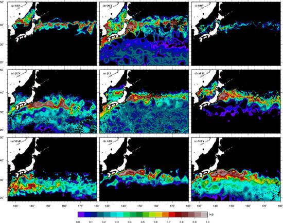
The TSS has been shown to provide a more robust measure of performance than the other three metrics that we calculated, particularly the AUC [25,59]. Given that the method to select algorithms to create an ensemble is still a gray area, we chose to use a metric that has been shown to work better in previous studies [22]. We constructed ensemble maps from all the 17 algorithms for each month, using the TSS as a weighting factor [22]. This approach gave higher statistical weights to algorithms whose TSS values were high, and lower weights to algorithms whose TSS values were low. The analysis workflow is illustrated in Figure 2.

3. Results

Our averaged model performance results for the monthly models for March to November, constructed using 17 algorithms are shown in Figure 3, in which the AUC, COR, TSS and Kappa statistics for many of the algorithms indicate good model performance. The Support Vector Machine (SVM), Boosted Regression Trees (BRT), Random Forests (RF), Multivariate Adaptive Regression Splines (MARS), Generalized Additive Models (GAM), Classification and Regression Trees (CART), Multi-layer Perceptron (MLP), Recursive Partitioning and Regression Trees (RPART), and Maximum Entropy (MAXENT) algorithms showed high performance consistently in all 9 months. However, the Flexible Discriminant Analysis (FDA), Mixture Discriminant Analysis (MDA), Bioclim (BIOC), Domain (DOM), Maxlike (MAXL), Mahalanobis Distance (MAHA) and Radial Basis Function (RBF) algorithms exhibited low model performance in some of the months, especially when the COR and Kappa metrics are considered (e.g., Figure 3d–f and 3h–i). The AUC statistic also shows high model performance for all algorithms from March to November. The mean and standard deviations of the four performance metrics for all algorithms are shown in Table S1, and the TSS values are in bold print. The mean ROC plots for the 17 algorithms in each of the 9 monthly models are shown in Figure S1, with confidence limits within 2 standard deviations of the mean. The ROC plots are probability plots of sensitivity (true positive rate) against 1-specificity (false positive rate) where an algorithm which presents a curve closer to the top-left corner indicates better performance compared to one where the curve is closer to the 45-degree line of the ROC space. For instance, the July ROC plots generated with the generalized linear model (GLM), FDA and MAXL (Figure S1:(5,68,104)) algorithms indicate ROC plots whose part of the plot lean towards the 45-degree line, hence lower performance. These results are quite different from the MAXENT ROC plots (Figure S1:(145–153)) for all the months, which illustrate higher performance. The variable response curves for SSC, SSHA and SST are shown in Figures S2, S3 and S4 respectively, where the values which influenced model performances are indicated by the peaks of each curve in a specific algorithm. However, there are algorithms which show relatively monotonic shapes for certain variables, e.g., the BRT and MAXL for the SSC, SSHA and SST variables. The shape, peak, and range of values around the peak present important information which influences the HSI map. Figure S5 illustrates the contribution of each variable in the respective model. These results illustrate the relative importance of each of the 3 variables used to construct the model, hence variables with high values on a plot indicate a relatively higher contribution by that variable to the model fit and HSI map, and vice-versa. Notable, for instance, is the importance of SSHA in the GLM, SVM, MLP and RPART algorithms between April and June, while SST shows a strong variable contribution in MAHA, MAXENT, MAXL, and BIOC between September and November. The ensemble HSI maps for March to November period are shown in Figure 4, which illustrates the aggregated map. The high value pixels (HSI>0.7) show a consistent pattern where the latitudinal displacement increases northward from March toward October and November.

4. Discussion

We modelled skipjack tuna habitats in the western North Pacific from March to November, using fishery data and satellite remotely sensed variables in 17 algorithms implemented in the sdm package [15]. Our approach employed ensemble modelling techniques drawn from correlative and machine-learning algorithms to generate an ensemble habitat prediction. This process enabled us to explore the inherent characteristics of each algorithm as well as the ensemble modeling approach for applications such as potential fishing zone forecasting and fishery management options. Given the collection of algorithms we applied, our work explores a much wider scope of habitat algorithms for skipjack tuna in this area than previously. Ensemble modelling has evolved from the need to aggregate outputs from different models, optimize the success rates while minimizing the variations and inherent modelling limitations of constituent models. Since models are representations of reality, and no single model can be perfect in estimating real world conditions, using a number of models is deemed an appropriate way of optimizing the true “signal” about the relationships a model is aiming to capture, and minimizing some “noise” created by errors and uncertainties in the data and the model structure [64]. Generally, consensus on the ideal method to aggregate outputs of single algorithms into an ensemble is still lacking. Some authors find simple averages adequate [64] while others use a threshold to select better performing algorithms first, followed by weighting of these map outputs into an ensemble [22,64,65]. Indeed, the intended use of an ensemble prediction may largely determine the aggregating method. Nevertheless, the practical applications (e.g., fishery and marine conservation) of ensemble model outputs are clear, and include reducing the likelihood of making decisions based on maps that are far from the ‘truth’, the costs of relying on a single algorithm prediction compared to an ensemble, and the benefits of using ensembles to explore the impacts of future phenomena such as fishery forecasts and impacts of climate change [66].
Our results showed that the performance of the 17 single algorithm models varied, with SVM, BRT, RF, MARS, GAM, CART, MLP, RPART, and MAXENT, showing consistently high performance in all the months (Figure 3). However, we also noted lower performance for FDA, MDA, BIOC, DOM, MAXL, MAHA and RBF algorithms in a number of months, particularly in May, July and August, October and November (Figure 3). Algorithm performance has been the subject of some studies, where some machine learning algorithms such as MAXENT and RF have been shown to outperform others [61,67]. In this work, four performance metrics were employed to measure algorithm performance, with the understanding that each metric measures different aspects of performance [67]. The COR metric for the MAHA algorithm was low in all months. However, previous work has shown that the TSS is a more reliable metric than the AUC, COR, and Kappa, because it is independent of prevalence and reflects true ecological phenomena rather than statistical artefacts [59,62], hence we relied on the TSS to generate ensemble predictions. Algorithm performance can be influenced by a number of factors, namely the inherent mathematical configuration, the environmental distribution of the data in the region of interest, in the training sample, and in regions that might be used for projection, as well as the input parameter settings [67]. For instance, it has been observed that MAXENT’s better performance in comparison to the other algorithms might be partly due to how the environmental variables and their interactions are modelled, where more mathematical complexity of the model is progressively improved when more data are available [68,69]. In other studies, it has been pointed out that generative methods such as MAXENT and RF render better results with small sample sizes, maybe due to faster convergence to their higher asymptotic error than discriminative methods [68]. By contrast, discriminative methods such as GLM and GAM improve their accuracy as the number of records increases and may even surpass results offered by generative methods at large sample sizes [68,70]. In this study, we provided all algorithms with the same input datasets and configurations as implemented in the sdm package and thus assessed the differences in output, which we largely attribute to the individual algorithm behavior. It is also worth noting that our results depict outputs of the currently implemented versions of the 17 algorithms as implemented in R, and it is likely that future updates of the algorithms may lead to variations in observed performance.
The response curves and variable importance plots (Figures S2, S3, S4 and S5) showed consistencies by some algorithms on the importance of either SST, SSC or SSHA over time. For instance, the GLM, SVM, MLP and RPART models showed that SSHA had a higher importance between March and June, while the RBF, MAHA, MAXL, DOM, BIOC and FDA placed higher variable importance on SST in May and June. By contrast, between September and November, a number of algorithms placed higher variable importance on SST and SSC. Visualizing the fitted functions of the various variables was important in exploring the modelled relationships, and also understanding the differences among the methods and how different fitted functions influenced mapped predictions [67]. From an ecological perspective, between March and June, skipjack tuna are abundant in the Kuroshio area, which is dominated by warm waters, as they advance north during the northward migration, hence the models may not have been sensitive to the SST signal as an important variable during this period, an observation made by earlier work [5]. However, as the fish migrated into the Kuroshio Oyashio Transition Zone (June–August), and later towards the Oyashio area (September–November) where the waters are cooler, the importance of SST was more apparent [8]. Skipjack tuna are warm water species, and the mechanisms with which they forage within warm waters along productive thermal and ocean color fronts are well explained in previous work [29,30,36,71]. Furthermore, it is worth noting that some algorithms did not do well at detecting responses on some variables, hence displayed monotonic response functions. For instance, the BRT and CART (March to June) algorithms showed a flat response for SSC in all months, yet other algorithms were able to pick that signal. A similar response was noted with the BRT algorithm for April, June, October and November, as well as the CART and MAXL algorithms between April and June. In another study which compared the performance of 6 algorithms (5 of which we also used), it was noted that individual models provided slightly different results with the same dataset [25]. This underscores the importance of multi-algorithm approaches, compared to relying entirely on single algorithm models [9,25].
The ensemble predictions (Figure 4) were created from a suite of 17 species distribution algorithms which were weighted with the TSS values (Table S1). We used the TSS weighting for creating ensemble predictions since there isn’t a clearly defined selection criteria and weighting metric for creating ensembles [22]. The TSS metric has been shown to be more reliable than the AUC, and to provide a more reasonable output in other studies [22,25]. In addition to these considerations, we also concur with [67] that the application for which an ensemble model is sought constitutes a fundamental question that shapes the choice and weighting of the single algorithms that create the ensemble prediction. The ensemble prediction maps aggregate the outputs of the individual algorithms, and are comparable in pattern to maps derived from previous work in the same area [5]. Furthermore, the observed northward displacement of high suitability indices from March to October is also consistent with recent descriptions of skipjack tuna migrations in the same area [36]. However, comparisons of ensemble outputs in a multi-year study could add more information on interannual variability of habitats. The foreseeable applications of our findings in the western North Pacific include potential fishing zone modelling and forecasting, and prediction of range shifts driven by climate change. Potential fishing zone forecasting comprises a much shorter time scale compared to climate change driven range shifts, but for both, it is important to understand how the algorithms perform when projected into new environmental spaces not sampled by the training data [67].
Our work was subject to a number of data and modelling limitations which we point out here for future consideration. First, we used a single-year fishery dataset as a response variable due to logistics related to data availability for this study. An inter-annual dataset using a multi-algorithm approach would have been more useful in elucidating the strengths and limitations of each algorithm, as well as the inter-annual variability in habitat characteristics as depicted by each algorithm. This would also have provided an opportunity for validations using an independent dataset as recommended by [9]. In addition, like any other field dataset, fishery-derived data are subject to sampling biases associated with sampling effort distribution, either influenced by fisherfolk choices or weather considerations, or both [26]. Second, our study used a set of 3 satellite-derived predictor variables (SST, SSC, SSHA) which we acknowledge are not the only environmental variables that are important for skipjack tuna habitat characterization. Indeed, other studies have also used variables such as oxygen concentration, currents, sub-surface temperatures and mixed layer depths [22,23,36]. We limited our work to only SSC, SST, SSHA since these are widely applied predictors in tuna habitat studies [7,72], which also enabled us manage the algorithm and predictor variable permutations in our runs. Third, all the response and predictor variable layers were standardized to ~25-km spatial resolution, monthly averaged files to create consistency in spatial-temporal resolutions, while cognizant of the fact that resolution trade-offs are often inevitable in species distribution modelling [26]. Therefore, it is possible to use a higher resolution dataset, especially for smaller areas where there is need to resolve fine-scale oceanographic features. Fourth, there are biases introduced by mismatches in space and time between the sampling protocols for the response and predictor variable datasets [20]. For example, while the fishery data were recorded at point spatial resolution, on a daily basis, for the purposes of this study, they were aggregated to ~25-km resolution to match the resolutions of the environmental predictors. At times, while temporal averaging to monthly timescales is deemed necessary to improve data coverage due to cloud cover (e.g., for SSC), it may hinder a model’s ability to resolve fine-scale daily to weekly signals that influence habitat characterization [5,26].

5. Conclusions

This work is a first attempt at a multi-algorithm species distribution habitat modelling for skipjack tuna in the western North Pacific, using presence-only response data and satellite-derived predictor variables. We draw the following conclusions within the confines of the datasets we used, the algorithms applied, and the input parameter settings of the algorithms applied in the study area. First, the multi-algorithm approach elucidated the strengths and weaknesses of the various algorithms to model and predict skipjack tuna habitats. According to the performance statistics, the SVM, BRT, RF, MARS, GAM, CART, MLP, RPART, and MAXENT achieved consistently better performance than other algorithms. Some of the lowest-performing algorithms were the FDA, MDA, BIOC, DOM, MAXL, MAHA and RBF, although this also varied in different months. Second, we found inter-algorithm variations in predictor variable responses, which we attributed to the inherent mathematical configuration of each algorithm. Consequently, it is important that the performance results and predictive ability of each algorithm are interpreted concurrently with the theoretical assumptions that were made in formulation of the algorithm. Third, we hesitate to ‘declare a winning’ algorithm but, on the contrary, emphasize that it is important for a user to determine the applications for which they require ensemble models for, and the questions they would want answered by the model results, hence to design an appropriate ensemble model. Subsequently, a user should evaluate the characteristics and parameter features of each algorithm in order to select an algorithm that is best suited to answer the desired questions.

Supplementary Materials

The following are available online at https://www.mdpi.com/2072-4292/12/16/2591/s1, Figure S1: Receiver operating characteristic (ROC) curves for 17 presence-only models, March to November. The continuous black line indicates the mean ROC for 10 runs while the dotted gray lines show 2 standard deviations of the mean. Figure S2: Mean response curves for SSC from 17 presence-only algorithms for 10 runs, March to November. Figure S3: Mean response curves for SSHA from 17 presence-only algorithms for 10 runs, March to November. Figure S4: Mean response curves for SST from 17 presence-only algorithms for 10 runs, March to November. Figure S5: Variable importance of SST, SSC, and SSHA over 9 months, using 17 presence-only algorithms. Table S1: Mean (color coded to emphasize high (green shade) and low (pink shade) values) and standard deviations of performance metrics for all algorithms. TSS values are in bold.

Author Contributions

R.M. and S.-I.S. conceptualized the study and worked on the methodology; R.M. analyzed the data, worked on the figures and wrote the first draft manuscript; S.-I.S. acquired the data, reviewed and edited the first draft manuscript. All authors have read and agreed to the published version of the manuscript.

Funding

This work was supported by the Research on Climate Change Adaptation (RECCA) Project of the Grant-in-Aid from the Japan’s Ministry of Education, Culture, Sports, Science and Technology (MEXT) and the Arctic Research Center, Hokkaido University.

Acknowledgments

The authors are grateful to the Research Program on Climate Change Adaptation (RECCA) Project and the Arctic Research Center, Hokkaido University for supporting this work. We acknowledge the use of Sea Surface Temperature data from the NCDC, the ocean color data distributed by NASA via the ocean color portal and the SSHA data from the BloomWatch 180 portal. Further, the authors appreciate Akira Nihira for providing the skipjack tuna catch dataset.

Conflicts of Interest

The authors declare no conflict of interest.

References

  1. Hutchinson, G.E. Concluding Remarks. Cold Spring Harb. Symp. Quant. Biol. 1957, 22, 415–427. [Google Scholar] [CrossRef]
  2. Vandermeer, J.H. Niche Theory. Annu. Rev. Ecol. Syst. 1972, 3, 107–132. [Google Scholar] [CrossRef]
  3. Hirzel, A.H.; Le Lay, G. Habitat suitability modelling and niche theory. J. Appl. Ecol. 2008, 45, 1372–1381. [Google Scholar] [CrossRef]
  4. Kobayashi, D.R.; Farman, R.; Polovina, J.J.; Parker, D.M.; Rice, M.; Balazs, G.H. ‘Going with the Flow’ or Not: Evidence of Positive Rheotaxis in Oceanic Juvenile Loggerhead Turtles (Caretta caretta) in the South Pacific Ocean Using Satellite Tags and Ocean Circulation Data. PLoS ONE 2014, 9, e103701. [Google Scholar] [CrossRef] [PubMed] [Green Version]
  5. Mugo, R.; Saitoh, S.-I.; Nihira, A.; Kuroyama, T. Habitat characteristics of skipjack tuna (Katsuwonus pelamis) in the western North Pacific: A remote sensing perspective. Fish. Oceanogr. 2010, 19, 382–396. [Google Scholar] [CrossRef]
  6. Zainuddin, M.; Kiyofuji, H.; Saitoh, K.; Saitoh, S.-I. Using multi-sensor satellite remote sensing and catch data to detect ocean hot spots for albacore (Thunnus alalunga) in the northwestern North Pacific. Deep Sea Res. Part II Top. Stud. Oceanogr. 2006, 53, 419–431. [Google Scholar] [CrossRef]
  7. Zainuddin, M.; Saitoh, K.; Saitoh, S.-I. Albacore (Thunnus alalunga) fishing ground in relation to oceanographic conditions in the western North Pacific Ocean using remotely sensed satellite data. Fish. Oceanogr. 2008, 17, 61–73. [Google Scholar] [CrossRef] [Green Version]
  8. Mugo, R.M.; Saitoh, S.-I.; Takahashi, F.; Nihira, A.; Kuroyama, T. Evaluating the role of fronts in habitat overlaps between cold and warm water species in the western North Pacific: A proof of concept. Deep Sea Res. Part II Top. Stud. Oceanogr. 2014, 107, 29–39. [Google Scholar] [CrossRef]
  9. Robinson, N.M.; Nelson, W.A.; Costello, M.J.; Sutherland, J.E.; Lundquist, C.J. A Systematic Review of Marine-Based Species Distribution Models (SDMs) with Recommendations for Best Practice. Front. Mar. Sci. 2017, 4, 421. [Google Scholar] [CrossRef] [Green Version]
  10. Thuiller, W.; Lafourcade, B.; Engler, R.; Araújo, M.B. BIOMOD—A platform for ensemble forecasting of species distributions. Ecography 2009, 32, 369–373. [Google Scholar] [CrossRef]
  11. Muñoz, M.E.D.S.; De Giovanni, R.; De Siqueira, M.F.; Sutton, T.; Brewer, P.; Pereira, R.S.; Canhos, D.A.L.; Canhos, V.P. openModeller: A generic approach to species’ potential distribution modelling. Geoinformatica 2009, 15, 111–135. [Google Scholar] [CrossRef]
  12. Guo, Q.; Liu, Y. ModEco: An integrated software package for ecological niche modeling. Ecography 2010, 33, 637–642. [Google Scholar] [CrossRef]
  13. Hijmans, R.J.; Elith, J. Species Distribution Modeling. 2016. Available online: https://rspatial.org/raster/sdm/index.html (accessed on 21 May 2020).
  14. Iturbide, M.; Bedia, J.; Herrera, S.; Del Hierro, O.; Pinto, M.; Gutiérrez, J.M. A framework for species distribution modelling with improved pseudo-absence generation. Ecol. Model. 2015, 312, 166–174. [Google Scholar] [CrossRef] [Green Version]
  15. Naimi, B.; Araújo, M.B. sdm: A reproducible and extensible R platform for species distribution modelling. Ecography 2016, 39, 368–375. [Google Scholar] [CrossRef] [Green Version]
  16. Kaschner, K.; Rius-Barile, J.; Kesner-Reyes, K.; Garilao, C.; Kullander, S.O.; Rees, T.; Froese, R. AquaMaps: Predicted Range Maps for Aquatic Species; World Wide Web Electronic Publication. 2019. Available online: https://www.aquamaps.org/ (accessed on 21 May 2020).
  17. Kachelriess, D.; Wegmann, M.; Gollock, M.; Pettorelli, N. The application of remote sensing for marine protected area management. Ecol. Indic. 2014, 36, 169–177. [Google Scholar] [CrossRef]
  18. Jones, M.C.; Cheung, W.W.L. Multi-model ensemble projections of climate change effects on global marine biodiversity. ICES J. Mar. Sci. 2014, 72, 741–752. [Google Scholar] [CrossRef] [Green Version]
  19. Byrne, M.; Gall, M.; Wolfe, K.; Agüera, A. From pole to pole: The potential for the Arctic seastar Asterias amurensis to invade a warming Southern Ocean. Glob. Chang. Biol. 2016, 22, 3874–3887. [Google Scholar] [CrossRef]
  20. Melo-Merino, S.M.; Reyes-Bonilla, H.; Lira-Noriega, A. Ecological niche models and species distribution models in marine environments: A literature review and spatial analysis of evidence. Ecol. Model. 2020, 415, 108837. [Google Scholar] [CrossRef]
  21. Zainuddin, M.; Farhum, A.; Safruddin, S.; Selamat, M.B.; Sudirman, S.; Nurdin, N.; Syamsuddin, M.; Ridwan, M.; Saitoh, S.-I. Detection of pelagic habitat hotspots for skipjack tuna in the Gulf of Bone-Flores Sea, southwestern Coral Triangle tuna, Indonesia. PLoS ONE 2017, 12, e0185601. [Google Scholar] [CrossRef] [Green Version]
  22. Alabia, I.D.; Saitoh, S.-I.; Igarashi, H.; Ishikawa, Y.; Usui, N.; Kamachi, M.; Awaji, T.; Seito, M. Ensemble squid habitat model using three-dimensional ocean data. ICES J. Mar. Sci. 2016, 73, 1863–1874. [Google Scholar] [CrossRef] [Green Version]
  23. Erauskin-Extramiana, M.; Arrizabalaga, H.; Hobday, A.J.; Cabré, A.; Ibaibarriaga, L.; Arregui, I.; Murua, H.; Chust, G. Large-scale distribution of tuna species in a warming ocean. Glob. Chang. Biol. 2019, 25, 2043–2060. [Google Scholar] [CrossRef] [PubMed] [Green Version]
  24. Báez, J.; Barbosa, A.M.; Pascual, P.; Ramos, M.L.; Abascal, F. Ensemble modeling of the potential distribution of the whale shark in the Atlantic Ocean. Ecol. Evol. 2019, 10, 175–184. [Google Scholar] [CrossRef] [PubMed]
  25. Shabani, F.; Kumar, L.; Ahmadi, M. A comparison of absolute performance of different correlative and mechanistic species distribution models in an independent area. Ecol. Evol. 2016, 6, 5973–5986. [Google Scholar] [CrossRef] [PubMed] [Green Version]
  26. He, K.S.; Bradley, B.A.; Cord, A.F.; Rocchini, D.; Tuanmu, M.-N.; Schmidtlein, S.; Turner, W.; Wegmann, M.; Pettorelli, N. Will remote sensing shape the next generation of species distribution models? Remote Sens. Ecol. Conserv. 2015, 1, 4–18. [Google Scholar] [CrossRef] [Green Version]
  27. Turner, W. Sensing biodiversity. Science 2014, 346, 301–302. [Google Scholar] [CrossRef]
  28. Wild, A.; Hampton, J. A review of the biology and fisheries for skipjack tuna, Katsuwonus pelamis, in the Pacific Ocean. FAO Fish. Tech. Pap. 1994, 336, 1–151. [Google Scholar]
  29. Nihira, A. Studies on the behavioral ecology and physiology of migratory fish schools of skipjack tuna (Katsuwonus pelamis) in the oceanic frontal area [Japan]. Bull. Tohoku Natl. Fish. Res. Inst. 1996, 58, 137–233. [Google Scholar]
  30. Saitoh, S.; Kosaka, S.; Iisaka, J. Satellite infrared observations of Kuroshio warm-core rings and their application to study of Pacific saury migration. Deep Sea Res. Part A Oceanogr. Res. Pap. 1986, 33, 1601–1615. [Google Scholar] [CrossRef]
  31. Sugimoto, T.; Tameishi, H. Warm-core rings, streamers and their role on the fishing ground formation around Japan. Deep Sea Res. Part A Oceanogr. Res. Pap. 1992, 39, S183–S201. [Google Scholar] [CrossRef]
  32. Sund, P.N.; Blackburn, M.; Williams, F. Tunas and their environment in the Pacific Ocean: A review. Oceanogr. Mar. Biol. Ann. Rev. 1981, 19, 443–512. [Google Scholar]
  33. Madureira, L.S.P.; Coletto, J.L.; Pinho, M.P.; Weigert, S.C.; Varela, C.M.; Campello, M.E.S.; Llopart, A. Skipjack (Katsuwonus pelamis) fishery improvement project: From satellite and 3D oceanographic models to acoustics, towards predator-prey landscapes. In Proceedings of the 2017 IEEE/OES Acoustics in Underwater Geosciences Symposium (RIO Acoustics), Rio de Janeiro, Brazil, 25–27 July 2017; pp. 1–7. [Google Scholar] [CrossRef]
  34. Nakamura, E.L. Food and Feeding Habits of Skipjack Tuna (Katsuwonus pelamis) from the Marquesas and Tuamotu Islands. Trans. Am. Fish. Soc. 1965, 94, 236–242. [Google Scholar] [CrossRef]
  35. Iizuka, K.; Asano, M.; Naganuma, A. Feeding habits of skipjack tuna (Katsuwonus pelamis Linnaeus) caught by pole and line and the state of young skipjack tuna distribution in the tropical seas of the Western Pacific Ocean. Bull. Tohoku Reg. Fish. Res. Lab. 1989, 51, 107–116. [Google Scholar]
  36. Kiyofuji, H.; Aoki, Y.; Kinoshita, J.; Okamoto, S.; Masujima, M.; Matsumoto, T.; Fujioka, K.; Ogata, R.; Nakao, T.; Sugimoto, N.; et al. Northward migration dynamics of skipjack tuna (Katsuwonus pelamis) associated with the lower thermal limit in the western Pacific Ocean. Prog. Oceanogr. 2019, 175, 55–67. [Google Scholar] [CrossRef]
  37. Ogura, M. Swimming Behavior of Skipjack, Katsuwonus pelamis, Observed by the Data Storage Tag at the Northwestern Pacific, Off Northern Japan, in Summer of 2001 and 2002; SCTB16 Working Paper; National Research Institute of Far Seas Fisheries: Shizuoka, Japan, 2003; Volume 16, pp. 1–10. Available online: http://wwwx.spc.int/coastfish/Sections/reef/Library/Meetings/SCTB/16/SKJ_7.pdf (accessed on 24 April 2020).
  38. Schaefer, K.M.; Fuller, D.W. Vertical movement patterns of skipjack tuna (Katsuwonus pelamis) in the eastern equatorial Pacific Ocean, as revealed with archival tags. Fish. Bull. 2007, 105, 379–389. [Google Scholar]
  39. Saitoh, S.; Chassot, E.; Dwivedi, R.; Fonteneau, A.; Kiyofuji, H.; Kumari, B. Remote Sensing Applications to Fish Harvesting. In Remote Sensing in Fisheries and Aquaculture; IOCCG: Dartmouth, NS, Canada, 2009; Volume 8. [Google Scholar]
  40. Fujino, K. Range of the skipjack tuna sub-population in the western Pacific Ocean. In Proceedings of the Second Symposium on the Results of the Cooperative Study of the Kuroshio and Adjacent Region, Tokyo, Japan, 28 September–1 October 1972; pp. 373–384. [Google Scholar]
  41. Matsumoto, W.M. Distribution, Relative Abundance and Movement of Skipjack Tuna, Katsuwonus pelamis, in the Pacific Ocean Based on Japanese Tuna Longline Catches 1964–67; NOAA Technical Report, NMFS SSRF; National Marine Fisheries Service: Seattle, Washington, USA, 1975; Volume 695, pp. 1–30.
  42. Akiyama, H.; Hidaka, K.; Hirai, M.; Ishida, Y.; Moku, M.; Sugimoto, S. Oyashio and Kuroshio. In Marine Ecosystems of the North Pacific; Perry, R.I., Mckinnell, S.M., Eds.; PICES: Sidney, BC, Canada, 2004; Volume 1, pp. 113–127. [Google Scholar]
  43. Yasuda, I. Hydrographic Structure and Variability in the Kuroshio-Oyashio Transition Area. J. Oceanogr. 2003, 59, 389–402. [Google Scholar] [CrossRef]
  44. Sakurai, Y. An overview of the Oyashio ecosystem. Deep Sea Res. Part II Top. Stud. Oceanogr. 2007, 54, 2526–2542. [Google Scholar] [CrossRef] [Green Version]
  45. Kawai, H. Hydrography of the Kuroshio Extension. In Kuroshio, Its Physical Aspects; University of Tokyo Press: Tokyo, Japan, 1972; pp. 235–352. [Google Scholar]
  46. Talley, L.D.; Nagata, Y.; Fujimura, M.; Iwao, T.; Kono, T.; Inagake, D.; Hirai, M.; Okuda, K. North Pacific Intermediate Water in the Kuroshio/Oyashio Mixed Water Region. J. Phys. Oceanogr. 1995, 25, 475–501. [Google Scholar] [CrossRef] [Green Version]
  47. Yasuda, I.; Okuda, K.; Hirai, M. Evolution of a Kuroshio warm-core ring—Variability of the hydrographic structure. Deep Sea Res. Part A Oceanogr. Res. Pap. 1992, 39, S131–S161. [Google Scholar] [CrossRef]
  48. Seki, M.P.; Flint, E.N.; Howell, E.; Ichii, T.; Polovina, J.J.; Yatsu, A. Transition Zone. In Marine Ecosystems of the North Pacific; PICES: Sidney, BC, Canada, 2004; Volume 1, pp. 201–209. [Google Scholar]
  49. Tameishi, H. Understanding Japanese sardine migrations using acoustic and other aids. ICES J. Mar. Sci. 1996, 53, 167–171. [Google Scholar] [CrossRef]
  50. Hirzel, A.H.; Hausser, J.; Chessel, D.; Perrin, N. Ecological Niche Factor Analysis: How to compute habitat suitability maps without absence data? Ecology 2002, 83, 2027–2036. [Google Scholar] [CrossRef]
  51. Wilson, C.; Morales, J.; Nayak, S.; Asanuma, I.; Feldman, G. Ocean-color radiometry and fisheries. In Why Ocean Colour? The Societal Benefits of Ocean-Colour Technology; Reports of the International Ocean-Colour Coordinating Group; IOCCG: Dartmouth, NS, Canada, 2008; pp. 47–57. [Google Scholar]
  52. Mueller, J.L. SeaWiFS algorithm for the diffuse attenuation coefficient, K(490), using water-leaving radiances at 490 and 555 nm. In SeaWiFS Postlaunch Technical Report Series: Volume 11; Technical Report; NASA Goddard Space Flight Center: Greenbelt, MD, USA, 2000; Volume 11, pp. 24–27. [Google Scholar]
  53. Takahashi, W.; Kawamura, H. Detection method of the Kuroshio front using the satellite-derived chlorophyll-a images. Remote Sens. Environ. 2005, 97, 83–91. [Google Scholar] [CrossRef]
  54. Ayers, J.M.; Lozier, M.S. Physical controls on the seasonal migration of the North Pacific transition zone chlorophyll front. J. Geophys. Res. 2010, 115, 05001. [Google Scholar] [CrossRef] [Green Version]
  55. Baith, K.; Lindsay, R.; Fu, G.; McClain, C.R. Data analysis system developed for ocean color satellite sensors. Eos Trans. AGU 2001, 82, 202. [Google Scholar] [CrossRef]
  56. Wessel, P.; Luís, J.F.; Uieda, L.; Scharroo, R.; Wobbe, F.; Smith, W.; Tian, D. The Generic Mapping Tools Version 6. Geochem. Geophys. Geosyst. 2019, 20, 5556–5564. [Google Scholar] [CrossRef] [Green Version]
  57. Chen, W.; Pourghasemi, H.R.; Zhang, S.; Wang, J.A. Comparative Study of Functional Data Analysis and Generalized Linear Model Data-Mining Techniques for Landslide Spatial Modeling. In Spatial Modeling in GIS and R for Earth and Environmental Sciences; Elsevier: Amsterdam, The Netherlands, 2019; pp. 467–484. [Google Scholar]
  58. De La Hoz, C.F.; Ramos, E.; Puente, A.; Juanes, J.A. Climate change induced range shifts in seaweeds distributions in Europe. Mar. Environ. Res. 2019, 148, 1–11. [Google Scholar] [CrossRef]
  59. Shabani, F.; Kumar, L.; Ahmadi, M. Assessing Accuracy Methods of Species Distribution Models: AUC, Specificity, Sensitivity and the True Skill Statistic. Acta Sci. Hum. Soc. Sci. 2018, 18, 7–18. [Google Scholar]
  60. Hanley, J.A.; McNeil, B.J. The meaning and use of the area under a Receiver Operating Characteristic (ROC) curve. Radiology 1982, 143, 29–36. [Google Scholar] [CrossRef] [Green Version]
  61. Elith, J.; Graham, C.; Anderson, R.P.; Dudík, M.; Ferrier, S.; Guisan, A.; Hijmans, R.; Huettmann, F.; Leathwick, J.R.; Lehmann, A.; et al. Novel methods improve prediction of species’ distributions from occurrence data. Ecography 2006, 29, 129–151. [Google Scholar] [CrossRef] [Green Version]
  62. Allouche, O.; Tsoar, A.; Kadmon, R. Kadmon Assessing the accuracy of species distribution models: Prevalence, kappa and the true skill statistic (TSS): Assessing the accuracy of distribution models. J. Appl. Ecol. 2006, 43, 1223–1232. [Google Scholar] [CrossRef]
  63. Cohen, J. A Coefficient of Agreement for Nominal Scales. Educ. Psychol. Meas. 1960, 20, 37–46. [Google Scholar] [CrossRef]
  64. Hao, T.; Elith, J.; Guillera-Arroita, G.; Lahoz-Monfort, J.J. A review of evidence about use and performance of species distribution modelling ensembles like BIOMOD. Divers. Distrib. 2019, 25, 839–852. [Google Scholar] [CrossRef]
  65. Zhang, Z.; Mammola, S.; Zhang, H. Does weighting presence records improve the performance of species distribution models? A test using fish larval stages in the Yangtze Estuary. Sci. Total Environ. 2020, 741, 140393. [Google Scholar] [CrossRef] [PubMed]
  66. Araujo, M.; New, M. Ensemble forecasting of species distributions. Trends Ecol. Evol. 2007, 22, 42–47. [Google Scholar] [CrossRef]
  67. Elith, J.; Graham, C. Do they? How do they? Why do they differ? On finding reasons for differing performances of species distribution models. Ecography 2009, 32, 66–77. [Google Scholar] [CrossRef]
  68. Aguirre-Gutiérrez, J.; Carvalheiro, L.G.; Polce, C.; Van Loon, E.E.; Raes, N.; Reemer, M.; Biesmeijer, J.C. Fit-for-Purpose: Species Distribution Model Performance Depends on Evaluation Criteria—Dutch Hoverflies as a Case Study. PLoS ONE 2013, 8, e63708. [Google Scholar] [CrossRef] [Green Version]
  69. Phillips, S.J.; Anderson, R.P.; Schapire, R.E. Maximum entropy modeling of species geographic distributions. Ecol. Model. 2006, 190, 231–259. [Google Scholar] [CrossRef] [Green Version]
  70. Phillips, S.J.; Dudík, M.; Elith, J.; Graham, C.; Lehmann, A.; Leathwick, J.; Ferrier, S. Sample selection bias and presence-only distribution models: Implications for background and pseudo-absence data. Ecol. Appl. 2009, 19, 181–197. [Google Scholar] [CrossRef] [Green Version]
  71. Druon, J.-N.; Chassot, E.; Murua, H.; Lopez, J. Skipjack Tuna Availability for Purse Seine Fisheries Is Driven by Suitable Feeding Habitat Dynamics in the Atlantic and Indian Oceans. Front. Mar. Sci. 2017, 4, 315. [Google Scholar] [CrossRef]
  72. Howell, E.A.; Hawn, D.R.; Polovina, J.J. Spatiotemporal variability in bigeye tuna (Thunnus obesus) dive behavior in the central North Pacific Ocean. Prog. Oceanogr. 2010, 86, 81–93. [Google Scholar] [CrossRef]
Figure 1. The study area, showing the western North Pacific (18–50° N and 120–180° E). The major currents and migration routes of skipjack tuna (redrawn after [29]).
Remotesensing 12 02591 g001
Figure 2. An illustration of the step by step analysis workflow implemented for our study.
Remotesensing 12 02591 g002
Figure 3. Averaged performance statistics (area under the curve (AUC), correlation coefficient (COR), true skill statistic (TSS), and Cohen’s kappa (Kappa)) for 10 runs from 17 presence-only algorithms, March to November.
Remotesensing 12 02591 g003
Figure 4. Ensemble habitat suitability maps created from 17 presence-only models for March to November, 2004.
Remotesensing 12 02591 g004
Table 1. Environmental data layers used, their resolutions and sources.
DataResolutionSourceAgency
SST-v2, AVHRR-AMSR-E0.25https://eclipse.ncdc.noaa.gov/pub/OI-daily-v2/IEEENOAA
SSC0.05https://oceancolor.gsfc.nasa.gov/l3/NASA
SSHA-global0.25https://coastwatch.pfeg.noaa.gov/coastwatch/CWBrowserWW180.jspNOAA
Table 2. Models used from the ‘sdm’ package and their dependent packages in R.
ID.ModelDependent PackageSource
01Generalized Linear Model (GLM)statshttps://www.rdocumentation.org/packages/stats
02Support Vector Machine (SVM)kernlabhttps://www.rdocumentation.org/packages/kernlab
03Boosted Regression Trees (BRT)gbmhttps://www.rdocumentation.org/packages/gbm
04Random Forests (RF)randomForesthttps://www.rdocumentation.org/packages/randomForest
05Multivariate Adaptive Regression Splines (MARS)earthhttps://www.rdocumentation.org/packages/earth
06Generalized Additive Models (GAM)mgcv; gamhttps://www.rdocumentation.org/packages/mgcv
07Classification and Regression trees (CART)treehttps://www.rdocumentation.org/packages/tree
08Flexible Discriminant Analysis (FDA)mdahttps://www.rdocumentation.org/packages/mda
09Mixture Discriminant Analysis (MDA)mdahttps://www.rdocumentation.org/packages/mda
10Bioclim (BIOC)dismohttps://www.rdocumentation.org/packages/dismo
11Domain (DOM)adehabitatHShttps://www.rdocumentation.org/packages/adehabitatHS
12Maxlike (MAXL)maxlikehttps://www.rdocumentation.org/packages/maxlike
13Mahalanobis Distance (MAHA)nonehttps://www.rdocumentation.org/packages/dismo
14Radial Basis Function (RBF)RSNNShttps://www.rdocumentation.org/packages/RSNNS
15Multi-Layer Perceptron (MLP)RSNNShttps://www.rdocumentation.org/packages/RSNNS
16Recursive Partitioning and Regression Trees (RPART)rparthttps://www.rdocumentation.org/packages/rpart
17Maximum Entropy (MAXENT)maxent.jarPhillips et al. 2006

