Extended Geometry and Probability Model for GNSS+ Constellation Performance Evaluation

Abstract

We proposed an extended geometry and probability model (EGAPM) to analyze the performance of various kinds of (Global Navigation Satellite System) GNSS+ constellation design scenarios in terms of satellite visibility and dilution of precision (DOP) et al. on global and regional scales. Different from conventional methods, requiring real or simulated satellite ephemerides, this new model only uses some basic parameters of one satellite constellation. Verified by the reference values derived from precise satellite ephemerides, the accuracy of visible satellite visibility estimation using EGAPM gets an accuracy better than 0.11 on average. Applying the EGAPM to evaluate the geometry distribution quality of the hybrid GNSS+ constellation, where highly eccentric orbits (HEO), quasi-zenith orbit (QZO), inclined geosynchronous orbit (IGSO), geostationary earth orbit (GEO), medium earth orbit (MEO), and also low earth orbit (LEO) satellites included, we analyze the overall performance quantities of different constellation configurations. Results show that QZO satellites perform slightly better in the Northern Hemisphere than IGSO satellites. HEO satellites can significantly improve constellation geometry distribution quality in the high latitude regions. With 5 HEO satellites included in the third-generation BeiDou navigation satellite system (BDS-3), the average VDOP (vertical DOP) of the 30° N–90° N region can be decreased by 16.65%, meanwhile satellite visibility can be increased by 38.76%. What is more, the inclusion of the polar LEO constellation can significantly improve GNSS service performance. When including with 288 LEO satellites, the overall DOPs (GDOP (geometric DOP), HDOP (horizontal DOP), PDOP (position DOP), TDOP (time DOP), and VDOP) are decreased by about 40%, and the satellite visibility can be increased by 183.99% relative to the Global Positioning System (GPS) constellation.

1. Introduction

Global Navigation Satellite System (GNSS) performance can be evaluated from several aspects, such as satellite signal quality [1,2], the precision of broadcast ephemerides [3,4,5], the multipath effect [6,7], convergence speed and precision of positioning [8,9]. Among all of these aspects, the satellite constellation, which defines the observation geometry distribution of navigation systems [10,11], is of fundamental importance, especially under the progress of constellation design. Satellite visibility and dilution of precision (DOP), which reflect the geometry distribution quality of constellations, is regarded as the metric that defines the mapping factor between the ranging error and positioning error [12,13].

With the development of the GNSS, the traditional Walker-delta constellation has been transformed into the hybrid constellation. In order to enhance the service in the area of the Asia-Pacific region (60° S–60° N, 50° E–170° E), the third-generation BeiDou navigation satellite system (BDS-3) constellation comprises a Walker constellation, inclined geosynchronous orbit (IGSO) constellation, and also the geostationary earth orbit (GEO) constellation, which dramatically improves the visible satellite number and DOP in the Asia-Pacific region [14]. Many researchers have analyzed the contribution of IGSO and GEO constellations for the BDS-3 [2,15].

However, the DOP of current GNSS constellations in high latitude areas is much larger than regions of middle and low latitude [15,16], which causes unfavorable positioning, navigation, and timing (PNT) performance in these areas. Meanwhile, the current coverage of the satellite-based augment system (SBAS) [17], relies on GEO satellites to broadcast the correction message, also lacks the continuous coverage of the polar regions. Besides, because the Arctic shipping routes are excepted to be the shortest and of considerable economic value from the Atlantic Ocean to Pacific Ocean [18], it is desirable to improve the satellite visibility and geometry distribution quality in high latitude areas, especially in the Arctic region. Therefore, given the facts mentioned above, highly eccentric orbits (HEO) satellites could be used [19]. Among these, the Russian Molniya satellites are the most common, which can be used to provide communication services for polar regions.

Conventional methods of satellite visibility and DOPs (GDOP (geometric DOP), HDOP (horizontal DOP), PDOP (position DOP), TDOP (time DOP), and VDOP (vertical DOP) ) assessment are based on real ephemerides [20] or simulated almanacs [21,22] after complex calculation. Wang et al. [16] proposed the geometry and probability model (GAPM) for the Global Positioning Satellite System (GPS) constellation. The GAPM method applies the concept of statistics to satellite visibility analysis and defines the satellite spatial distribution probability density function based on the satellite angular velocity. This method only requires some constellation parameters and dramatically reduces the calculation burden. This method was later used by Chen J. [23] to calculate the GNSS DOP of low earth orbit (LEO) satellites. However, GAPM is only suitable for the medium earth orbit (MEO) or LEO constellations, and to evaluate the contributions of IGSO and GEO satellites of BDS-3, Wang et al. [15] developed the modified GAPM (MGAPM) method. Through the constraint of the domain of a function to the ground track of IGSO or GEO satellites, MGAPM realizes the extension of GAPM. By revisiting their method and considering the GNSS+ constellation with possible non-circular HEO and quasi-zenith orbit (QZO), we present an extended and modified geometry and probability model (EGAPM) with the capability of analyzing the contribution of large eccentricity satellite orbit constellations to navigation performance. EGAPM is validated through the satellite visibility and DOP results compared with that of precise ephemerides of GPS and BDS-3+QZO. Meanwhile, LEO satellites enhancing GNSS would be one of the promising development trends in the future [24,25,26]; hence, we also evaluate the contribution of the polar LEO constellation to navigation. Besides, we assess the performance of the GNSS+ constellation with 30 BDS-3, 288 LEO, and 5 HEO satellites using the EGAPM and demonstrate its superiority to BDS-3 and GPS nominal constellations.

2. Methods

In the previous GAPM method [15,16], the observing sphere was divided into latitudes and longitudes grids by 1° × 1°, and the probability of a satellite appearing in one grid can be determined by its velocity. This probability is regarded as the satellite observing probability, which is the basis of the estimation of satellite visibility and DOP. For one specific station on the earth ellipsoid, the number of visible satellites is the sum of probability of the constellation in the observation area of the station. Furthermore, the satellite probability is regarded as weighting factors in the calculation of DOPs. Based on the DOPs, the performance and characterization of satellite visibility and geometry distribution for one GNSS constellation can be further evaluated. It is noted that the opportunities of a satellite’s appearance in certain areas are zero where the latitude is higher than the satellite’s orbit incline angle. Because the previous GAPM method is only applicable for the approximately circular orbit, we modify and extend the GAPM method in this paper to make it applicable for BDS-3 IGSO, QZO, and HEO satellites.

2.1. MEO and LEO Satellite Observing Probability

For GNSS MEO or LEO satellites in approximately circular orbits, previous GAPM is effective. The velocity of east-west direction $V_{\lambda }$ and north-south direction $V_{\phi }$ for the position ($\phi$,$\lambda$) can be written as [16]:

$$\{\begin{array}{l}{V}_{\lambda }=\sqrt{\frac{GM}{R}}\cdot \frac{\cos i_{orb}}{\cos \phi }\\ V_{\phi }=\sqrt{\frac{GM}{R}}\cdot \sqrt{1-{\left(\frac{\cos i_{orb}}{\cos \phi }\right)}^2}\end{array},$$

(1)

where GM is the product of the gravitational constant and the earth’s mass; R is the norm of a satellite position vector; i_orb is the satellite’s orbit incline angle to the equator; $\phi$ is geocentric latitude; $\lambda$ is longitude.

As Equation (1) shows, the velocity of satellites appearing in one grid element is a function related to the latitude. So, for satellites appearing in the grid elements with the same geocentric latitude, the $V_{\phi }$ term would be the same. Based on the hypothesis that GNSS satellites are distributed symmetrically in the east-west direction, the in and out satellites of the grid are balanced in this direction [15]. Therefore, the observing probability of a satellite depends on $V_{\phi }$ only. The satellite observing probability can be modified as [15]:

$$P^{M/L}=\{\begin{array}{c}\frac{k}{V_{\phi }}=\sqrt{\frac{R}{GM}}\frac{k\cos \phi }{\sqrt{{\cos }^2\phi -{\cos }^2{i}_{orb}}}\\ 0,\hspace{1em}\hspace{1em}|\phi |\ge i_{orb}\end{array},|\phi |<i_{orb},$$

(2)

where k is the probability constant for a specific GNSS MEO or LEO satellite constellation. The superscript M/L stands for GNSS MEO or LEO satellites.

As mentioned above, the spherical orbit surface can be divided into 1° × 1° grids centered in $({\phi }_i,{\lambda }_j)$:

$$\{\begin{array}{l}{\phi }_i=i-0.5\hspace{1em}i=-89,-88,\dots ,90\\ {\lambda }_j=j-0.5\hspace{1em}j=-179,-178,\dots ,180\end{array}.$$

(3)

In addition, the probability constant k can be calculated as [16]:

$$k=\frac{n}{{\displaystyle \sum _{i=-89}^{90}{\displaystyle \sum _{j=-179}^{180}\frac{1}{V_{\phi }}}}},$$

(4)

where n is the total number of GNSS MEO or LEO satellites.

2.2. GEO and IGSO Satellite Observing Probability

GEO satellites are relatively static to earth in earth-centered earth fixed (ECEF) system. Therefore, in theory, a GEO satellite will stay at the specific point all the time. For instance, the 3 BDS-3 GEO satellites are respectively located at 80° E, 110.5° E, and 140° E [27]. So, in theory, the probability of a GEO satellite appearing at the designed position, such as 80 ° E, is 1, while at other arbitrary positions is 0. Then GEO satellite observing probability can be written as [15]:

$$P_{\left(X,Y,Z\right)}^{GEO}=\{\begin{array}{l}1,\left(X,Y,Z\right)\in P\\ 0,other positions\end{array}.$$

(5)

For an IGSO satellite, their satellite ground track is a closed curve. For example, the 3 BDS-3 IGSO satellites, their ground tracks are coincident, while the longitude of the intersection point is at 118° E, with a phase difference of 120° [28]. We can calculate a satellite position (X, Y, Z) in the ECEF system when the true anomaly f turns a specific angle and the set of these points in one earth self-rotation period is called B in this study. For an IGSO satellite, when f turns over from 0° to 360°, all coordinates in the ECEF system and corresponding velocity in one earth self-rotation period can be obtained. Considering both the accuracy and computation efficiency, this specific angle can be set at 0.25° [15]. Then, refer to the idea of previous GAPM, the probability of IGSO satellites appearing at one point of B can be determined by the corresponding velocity. So, the modified probability definition, $P_{\left(X,Y,Z\right)}^{IGSO}$, of IGSO satellites to be observed at one point of B can be written as:

$$P_{\left(X,Y,Z\right)}^{IGSO}=\{\begin{array}{l}\frac{k^{IGSO}}{V_{{}_{\left(X,Y,Z\right)}}^{IGSO}},\left(X,Y,Z\right)\in \mathrm{B}\\ 0,other positions\end{array},$$

(6)

where $V_{{}_{\left(X,Y,Z\right)}}^{IGSO}$ is the velocity at one point of B in the ECEF system; k^IGSO is the probability constant for IGSO satellites which can be calculated by the following equation:

$$k^{IGSO}=\frac{n^{IGSO}}{{\displaystyle \sum _{\left(X,Y,Z\right)\in \mathrm{B}}\frac{1}{V_{\left(X,Y,Z\right)}^{IGSO}}}},$$

(7)

where n^IGSO is the total number of IGSO satellites with the same ground track. $V_{{}_{\left(X,Y,Z\right)}}^{IGSO}$ at one point of B can be calculated as follows. Firstly, a satellite position (X, Y, Z) in ECEF can be computed with the true anomaly f as the independent variable. Then, the velocity of X, Y, and Z components: V_X, V_Y, and V_Z can be written as:

$$\{\begin{array}{l}{V}_X=\frac{X_{t+\Delta t}-X_t}{\Delta t}\\ V_Y=\frac{Y_{t+\Delta t}-Y_t}{\Delta t}\\ V_Z=\frac{Z_{t+\Delta t}-Z_t}{\Delta t}\end{array},$$

(8)

where t is one specific epoch; X, Y, and Z are the ECEF coordinates of a satellite at the epoch t or t + Δt; Δt means the time elapsed from one point to another very adjacent point. Then, $V_{\left(X,Y,Z\right)}$ at one point is:

$$V_{{}_{\left(X,Y,Z\right)}}^{IGSO}=\sqrt{V_X^2+V_Y^2+V_Z^2}.$$

(9)

We investigate the observing probability of the three BDS-3 IGSO satellites using the modified observing probability definition of IGSO satellites. From Figure 1, it can be seen that the observing probability is larger at the northern and southern ends of the figure-8-shape track which is closer to the actual situation than the corresponding results presented in [15].

2.3. HEO and QZO Satellite Observing Probability

As mentioned above, LEO, MEO, GEO, and IGSO satellites are all in approximately circle orbits with small eccentricity, and the magnitude of satellites’ position vector and flight velocity vector are almost constant, which is the prerequisites for the earlier GAPM [15,16]. However, some special kinds of orbits have larger eccentricity, such as the QZO satellites of the Quasi-Zenith Satellite System (QZSS) [29]. The eccentricity of QZO satellites of about 0.075 is much larger than that of GPS satellites, which is normally less than 0.01. To investigate the performance of satellite orbits with large eccentricity, the traditional GAPM mentioned above should be generalized. For this purpose, the key issue is to calculate their space coordinates and corresponding velocity in the ECEF system. Therefore, some points need to be considered: (1) the magnitude of satellite position vector will change all the time; (2) the time that satellite fly from one point to another adjacent point is different because the satellite velocity and the magnitude of position vector are changing all the time; (3) the magnitude of satellite velocity in the ECEF system is changing also.

For point (1), the magnitude of satellite position vector R can be calculated by the following equation [19]:

$$R=\frac{a\left(1-e^2\right)}{1+e\cos f},$$

(10)

where e is the orbit eccentricity; a is semi-major axis. From Equation (10), we know that the R is the function of the true anomaly f.

For point (2), according to Kepler’s second law, the radius vector sweeps over equal areas in equal time intervals [19], i.e., the area rate $\dot{\mathrm{A}}$, is a constant:

$$\dot{\mathrm{A}}=\frac{\sqrt{aGM\left(1-e^2\right)}}{2}.$$

(11)

Therefore, the elapsed time for the satellite from one point to adjacent point can be calculated by the equation, $\mathrm{A}/\dot{\mathrm{A}}$, where A is the area that radius vector swept during the period. If the true anomaly changes by a very small amount and the area that the radius swept could be regarded as a circular sector, then the area of this tiny circular sector, dA, can be calculated by the following equation:

$$dA=\frac{1}{2}{R}^{2}df=\frac{1}{2}{\left(\frac{a\left(1-e^2\right)}{1+e\cos f}\right)}^{2}df,$$

(12)

where df is the tiny change of true anomaly. The whole area could then be derived by the area integral within the interval [f, f + 0.25°]:

$$A=\frac{1}{2}{\displaystyle {\int }_f^{f+{0.25}^{°}}{\left(\frac{a\left(1-e^2\right)}{1+e\cos f}\right)}^{2}df}.$$

(13)

However, the analytical expression of this integration is quite complex, and the result of numerical integration can be used. The interval [f, f + 0.25°] is divided into 10,000 pieces, and the above equation can be reformulated as:

$$A\approx \frac{1}{2}{\displaystyle \sum _{i=1}^{10000}{\left(\frac{a\left(1-e^2\right)}{1+e\cos \left(f+0.000025i\right)}\right)}^2\left(0.000025i\right)}.$$

(14)

Thus, the elapsed time, $\Delta t$, can be written as:

$$\Delta t\approx \frac{\mathrm{A}}{\dot{\mathrm{A}}}.$$

(15)

When $\Delta t$ is determined, satellite velocity in the ECEF system could be derived. Satellite coordinates in the orbital plane coordinate system can be written as:

$$\{\begin{array}{l}{\eta }_f=R\cos f\\ {\xi }_f=R\sin f\end{array},f=0,0.25,\dots ,360,\dots .,$$

(16)

where $\eta$ is the axis points to the ascending node and $\xi$ is the axis points to the direction on the argument of the latitude of 90°.

Satellite coordinates can be transformed from the orbital plane coordinate system into the ECEF system:

$$\left(\begin{array}{l}{X}_i\\ Y_i\\ Z_i\end{array}\right)=R_3\left(-{\mathsf{\Omega }}_i\right)R_1\left(-i_{orb}\right)\left(\begin{array}{l}{\eta }_i\\ {\xi }_i\\ 0\end{array}\right),$$

(17)

where $R_3(-{\mathsf{\Omega }}_i)$ and $R_1(-i_{orb})$ are rotation matrices as follows:

$$R_3\left(-{\mathsf{\Omega }}_i\right)=\left(\begin{array}{ccc}\cos {\mathsf{\Omega }}_i& -\sin {\mathsf{\Omega }}_i& 0\\ \sin {\mathsf{\Omega }}_i& \cos {\mathsf{\Omega }}_i& 0\\ 0& 0& 1\end{array}\right),$$

(18)

$$R_1\left(-i_{orb}\right)=\left(\begin{array}{ccc}1& 0& 0\\ 0& \cos i_{orb}& -\sin i_{orb}\\ 0& \sin i_{orb}& \cos i_{orb}\end{array}\right),$$

(19)

where ${\mathsf{\Omega }}_i$ is the right ascension of ascending node which can be written as:

$${\mathsf{\Omega }}_i=\left({\mathsf{\Omega }}_0-\Delta t\cdot {\omega }_{earth}\right)\frac{\pi }{{180}^{°}},$$

(20)

where ${\mathsf{\Omega }}_0$ is the right ascending node at the initial epoch; ${\omega }_{earth}$ is the angular velocity of the earth rotation. $\Delta t$ can be obtained by Equation (15). Thus, all ECEF cartesian coordinates in one earth rotation period can be calculated and the set of these coordinates is defined as $\mathsf{\Gamma }$.

As for point (3), the magnitude of satellite velocity in the ECEF system can be calculated using the Equations (8) and (9).

Finally, the observing probability of a satellite at one point of $\mathsf{\Gamma }$ can be written as:

$$P_{\left(X,Y,Z\right)}^{HEO/QZO}=\{\begin{array}{l}\frac{k^{HEO/QZO}}{V_{{}_{\left(X,Y,Z\right)}}^{HEO/QZO}},\left(X,Y,Z\right)\in \mathsf{\Gamma }\\ 0,other positions\end{array},$$

(21)

where the superscript HEO/QZO stands for HEO or QZO satellites; $k^{HEO/QZO}$ is the corresponding probability constant for HEO or QZO satellites of large eccentricity orbits with the same ground track, which can be written as:

$$k^{HEO/QZO}=\frac{n^{HEO/QZO}}{{\displaystyle \sum _{\left(X,Y,Z\right)\in \mathsf{\Gamma }}\frac{1}{V_{{}_{\left(X,Y,Z\right)}}^{HEO/QZO}}}},$$

(22)

where $n^{HEO/QZO}$ is the total number of HEO or QZO satellites with the same ground track; $V_{{}_{(X,Y,Z)}}^{HEO/QZO}$ is the velocity of HEO or QZO at one point of $\mathsf{\Gamma }$ in the ECEF system.

Based on the mentioned above, observing the probability distribution of 3 QZO satellites can be seen from Figure 2. The eccentricity of QZO is set as 0.075, but the inclination and the center of the longitude of the ground track are the same as IGSO of BDS-3. The distribution shows that the probability is larger at the northern end of the track, which is very different from IGSO satellites, as a consequence of the velocity near apogee being lower.

2.4. Calculation of DOPs and Satellite Visibility

A satellite is visible when it is above a specific cutoff elevation angle (CEA). In this paper, to ensure higher accuracy, we apply the 5° CEA for the following DOP and satellite visibility calculations [15]. We calculated the probability for each satellite that the satellite elevation angle is higher than CEA for each grid element. Then the visible satellite number N can be written as:

$$\begin{array}{ll}N=& {\displaystyle \sum _{i=-89}^{90}{\displaystyle \sum _{j=-179}^{180}{P}_{ij}^{MEO}}+}{\displaystyle \sum _{i=-89}^{90}{\displaystyle \sum _{j=-179}^{180}{P}_{ij}^{LEO}}+}{\displaystyle \sum _{i=-89}^{90}{\displaystyle \sum _{j=-179}^{180}{P}_{ij}^{HEO}}}+\\ & {\displaystyle \sum _{i=-89}^{90}{\displaystyle \sum _{j=-179}^{180}{P}_{ij}^{IGSO}}+{\displaystyle \sum _{i=-89}^{90}{\displaystyle \sum _{j=-179}^{180}{P}_{ij}^{GEO}}}}+{\displaystyle \sum _{i=-89}^{90}{\displaystyle \sum _{j=-179}^{180}{P}_{ij}^{QZO}}}\end{array}.$$

(23)

The observation equation of a satellite can be written as [27]:

$$v=\left(e_x{e}_y{e}_{z}1\right)\left(\begin{array}{l}\delta X\\ \delta Y\\ \delta Z\\ c\delta t\end{array}\right)-l,$$

(24)

where e_x, e_y, and e_z are the unit vectors of station-to-satellite vector; v is the residual; $c\delta t$ the receiver clock correction; l is the vector of observations; $\delta X$, $\delta Y$, and $\delta Z$ are the corrections to a station’s approximate coordinates. In EGAPM, observation equations can be established for each grid or point higher than specific CEA and corresponding probability is regarded as its weight. Then, using the above information, for an arbitrary station on the earth ellipsoid, the coefficient matrix of the normal equations can be written as [16]:

$$Nbb=\left(\begin{array}{cccc}\hfill {\displaystyle \sum _{i=-89}^{90}{\displaystyle \sum _{j=-179}^{180}{P}_{ij}{e}_x^2}{|}_D }& \hfill {\displaystyle \sum _{i=-89}^{90}{\displaystyle \sum _{j=-179}^{180}{P}_{ij}{e}_x{e}_y}{|}_D }& \hfill {\displaystyle \sum _{i=-89}^{90}{\displaystyle \sum _{j=-179}^{180}{P}_{ij}{e}_x{e}_z}{|}_D }& \hfill {\displaystyle \sum _{i=-89}^{90}{\displaystyle \sum _{j=-179}^{180}{P}_{ij}{e}_{{}_x}}{|}_D }\\ \hfill & \hfill {\displaystyle \sum _{i=-89}^{90}{\displaystyle \sum _{j=-179}^{180}{P}_{ij}{e}_y^2}{|}_D}& \hfill {\displaystyle \sum _{i=-89}^{90}{\displaystyle \sum _{j=-179}^{180}{P}_{ij}{e}_y{e}_{{}_z}}{|}_D }& \hfill {\displaystyle \sum _{i=-89}^{90}{\displaystyle \sum _{j=-179}^{180}{P}_{ij}{e}_y}{|}_D }\\ \hfill & \hfill & \hfill {\displaystyle \sum _{i=-89}^{90}{\displaystyle \sum _{j=-179}^{180}{P}_{ij}{e}_x^2}{|}_D}& \hfill {\displaystyle \sum _{i=-89}^{90}{\displaystyle \sum _{j=-179}^{180}{P}_{ij}{e}_z}{|}_D }\\ \mathrm{symmetry}\hfill & \hfill & \hfill & \hfill {\displaystyle \sum _{i=-89}^{90}{\displaystyle \sum _{j=-179}^{180}{P}_{ij}}{|}_D }\end{array}\right),$$

(25)

where D is the visible area above CEA.

The inverse of the normal equation in Equation (25) gives the variance/covariance matrix Q:

$$Q=Nb{b}^{{}^{-1}}.$$

(26)

Then, the geometric dilution of precision, GDOP, by definition, is the square root of the trace of the variance/covariance matrix Q.

Cartesian coordinates can be translated into the station’s topocentric up (U), north (N), and east (E) coordinate system using the following equations:

$$\left(\begin{array}{c}\delta X\\ \delta Y\\ \delta Z\\ c\delta t\end{array}\right)=\left(\begin{array}{cc}\frac{\partial \left(\begin{array}{ccc}X& Y& Z\end{array}\right)}{\partial \left(\begin{array}{ccc}U& E& N\end{array}\right)}& 0\\ 0& 1\end{array}\right)\left(\begin{array}{c}\delta U\\ \delta E\\ \delta N\\ c\delta t\end{array}\right)=S\left(\begin{array}{c}\delta U\\ \delta E\\ \delta N\\ c\delta t\end{array}\right),$$

(27)

$$\frac{\partial \left(\begin{array}{ccc}X& Y& Z\end{array}\right)}{\partial \left(\begin{array}{ccc}U& E& N\end{array}\right)}=R_2\left(\text{-}B\right)R_3\left(L\right),$$

(28)

where $R_3\left(-L\right)$ and $R_2\left(B\right)$ are rotation matrices which can be written as follow:

$$R_3\left(L\right)=\left(\begin{array}{ccc}\cos \left(L\right)& \sin \left(L\right)& 0\\ -\sin \left(L\right)& \cos \left(L\right)& 0\\ 0& 0& 1\end{array}\right),$$

(29)

$$R_2\left(-B\right)=\left(\begin{array}{ccc}\cos \left(-B\right)& 0& -\sin \left(-B\right)\\ 0& 1& 0\\ \sin \left(-B\right)& 0& \cos \left(-B\right)\end{array}\right).$$

(30)

Then, the normal equation can be written as:

$$N_{{}_{BLh}}=S^{{}^T}NS.$$

(31)

In addition, the covariance matrix Q_UEN can be derived using the variance propagation rule as:

$$Q_{{}_{UEN}}={\left(S^{{}^T}NS\right)}^{\text{-}1}.$$

(32)

So, by definition, the DOPs can be written as:

$$\{\begin{array}{l}PDOP=\sqrt{Q_{UEN}\left(1,1\right)+Q_{UEN}\left(2,2\right)+Q_{UEN}\left(3,3\right)} position DOP\hfill \\ HDOP=\sqrt{Q_{UEN}\left(2,2\right)+Q_{UEN}\left(3,3\right)} horizontal DOP\hfill \\ VDOP=\sqrt{Q_{UEN}\left(1,1\right)} vertical DOP\hfill \\ \begin{array}{l}TDOP=\sqrt{Q_{UEN}\left(4,4\right)} time DOP\\ NDOP=\sqrt{Q_{{}_{{}_{UEN}}}\left(3,3\right)} north DOP\\ EDOP=\sqrt{Q_{UEN}\left(2,2\right)} east DOP\end{array}\hfill \end{array}.$$

(33)

Obtained from the above expression, the correlation, ${\rho }_{Uclk}$, of station geodetic height between receiver clock difference follows the expression of:

$${\rho }_{Uclk}=\frac{Q_{BUEN}\left(1,4\right)}{\sqrt{Q_{UEN}\left(1,1\right)}\sqrt{Q_{UEN}\left(4,4\right)}}.$$

(34)

In addition, the ratio, NE, of the positioning precision in the longitude component to the latitude component can be written as:

$$NE=\frac{\sqrt{Q_{UEN}\left(3,3\right)}}{\sqrt{Q_{UEN}\left(2,2\right)}}.$$

(35)

In summary, we can establish an observation equation based on all grids or points above CEA, and the probability of satellites in this grid is regarded as the weight of this observation equation. Then, the normal equation of the GNSS+ constellation can be given by:

$$N_{bb}^{GNSS+}=N_{bb}^{MEO}+N_{bb}^{LEO}+N_{bb}^{GEO}+N_{bb}^{IGSO}+N_{bb}^{HEO}+N_{bb}^{QZO},$$

(36)

where $N_{bb}^{MEO}$, $N_{bb}^{LEO}$, $N_{bb}^{GEO}$, $N_{bb}^{IGSO}$, $N_{bb}^{QZO}$, and $N_{bb}^{HEO}$ can be given by Equation (25).

3. Method Validation

We used 24 h averages on global scales of the values derived from real GPS precise ephemerides provided by GeoForschungsZentrum Potsdam (GFZ) and the precise ephemerides of the BDS-3+QZO simulation constellation, to validate the usefulness EGAPM and assess the method of satellite visibility and DOPs estimation. Constellation parameters of BDS-3+QZO and GPS are shown in

Table 1. Constellation parameters of third-generation BeiDou navigation satellite system (BDS-3)+ Quasi-Zenith orbit (QZO) and Global Positioning System (GPS) [28,29,30].

Parameter	BDS-3+QZO			GPS
Orbit Type	MEO	QZO	GEO	MEO
Nominal Number	24	3	3	32
Inclination	55°	55°	0°	55°
Altitude (KM)	21,528	38,950.6 (Apogee)	35,786	20,200
Period(s)	46,404	86,170.5	86,170.5	43,080

.

Estimations of the number of visible satellites and corresponding reference values at 5° CEA are shown in Figure 3. Using EGAPM, the root mean squares (RMS) between the estimated and reference number of visible satellites are 0.10 for 32 GPS satellites and 0.05 for 30 BDS-3+QZO satellites. Generally, the discrepancies between estimated and reference values at high latitudes are larger than other locations.

The underestimating rates for the GPS and BDS-3+QZO constellation are calculated (

Table 2. Average, minimal, and maximal underestimating rates of the estimated GPS and BDS-3+QZO DOPs ((GDOP (geometric DOP), HDOP (horizontal DOP), PDOP (position DOP), TDOP (time DOP), and VDOP (vertical DOP) )) relative to the reference values ((reference-estimation)/reference × 100%) over latitudes.

Constellation	Underestimating Rates of DOPs (%)
	Average (Min–Max)
	GDOP	PDOP	HDOP	VDOP
GPS	10.41 (5.06–13.10)	9.85 (4.58–12.40)	7.98 (3.96–10.63)	10.33 (4.64–13.03)
BDS-3+QZO	10.94 (6.93–16.12)	10.39 (6.46–15.09)	7.95 (4.44–10.55)	11.07 (6.79–16.91)

), to assess the DOPs underestimation with a 5° CEA. The average underestimating rates are 7.95–11.07%.

4. Experimental Results and Analyses

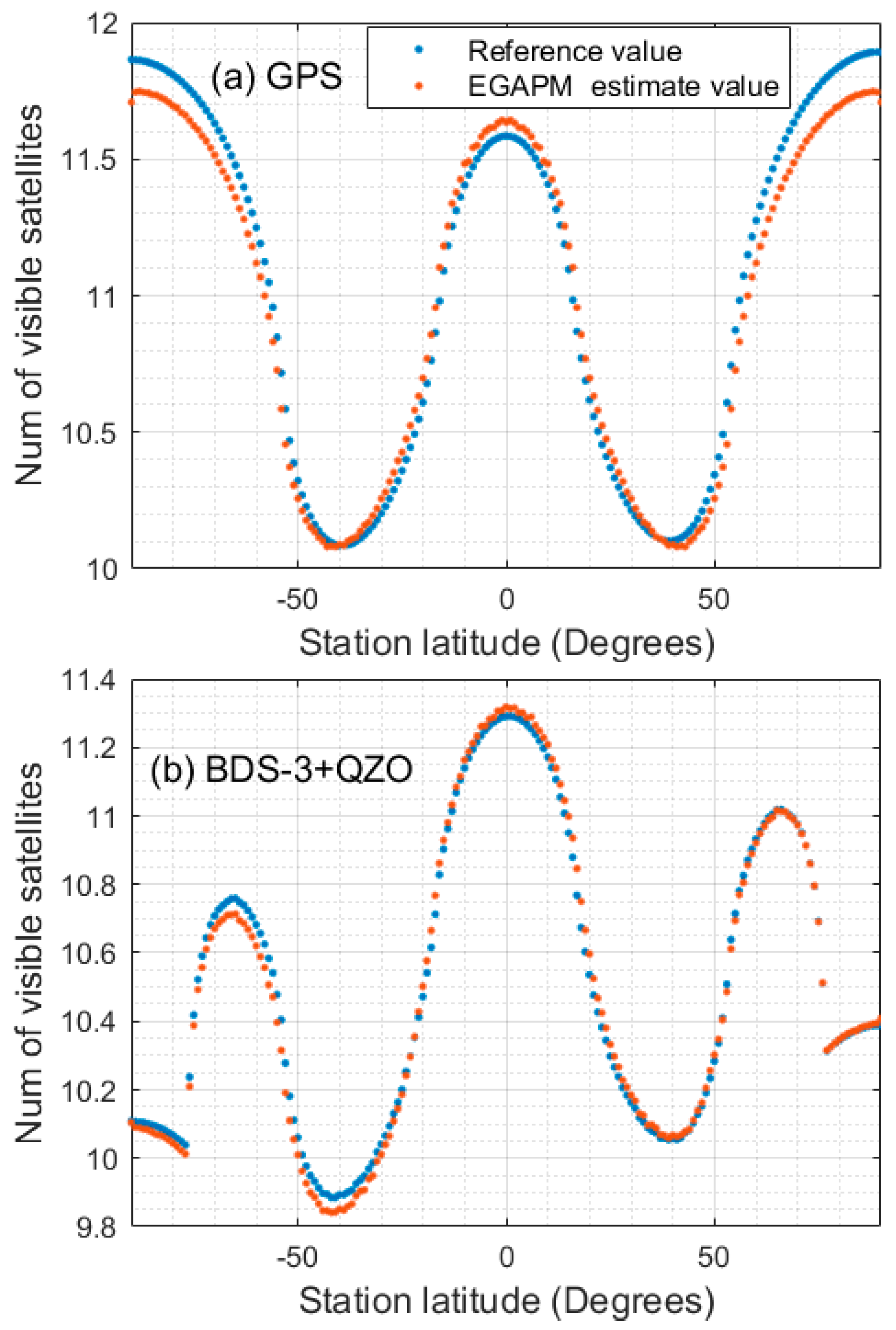
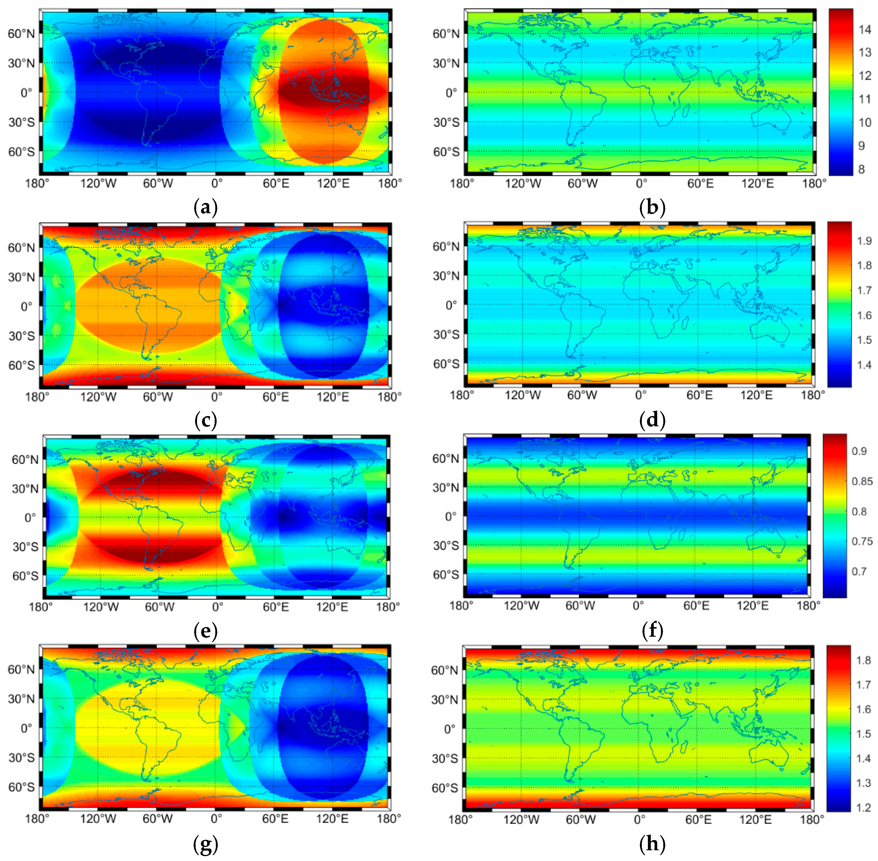
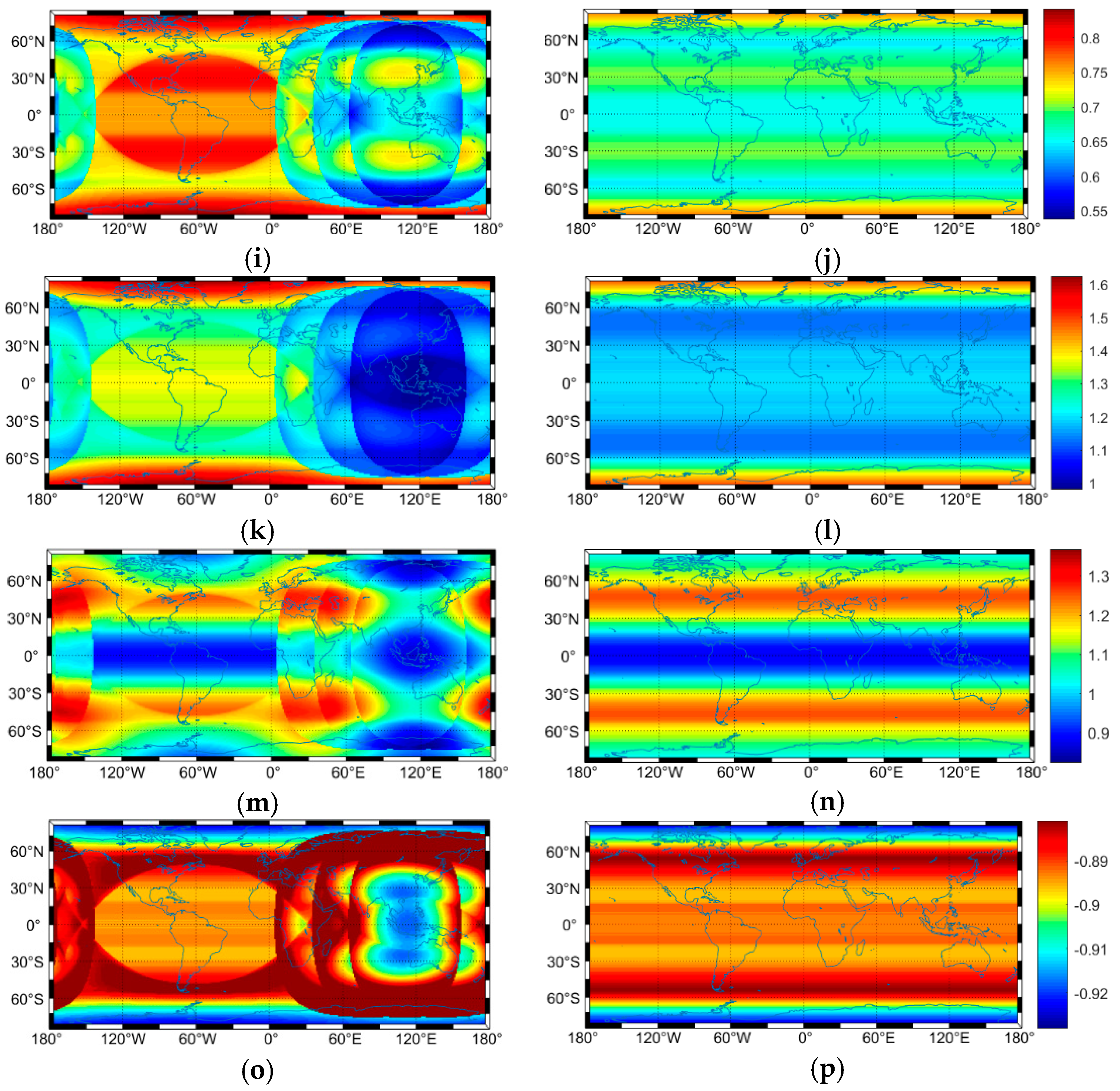
In this section, the satellite visibility and geometry distribution quality of GNSS and GNSS+ constellations are investigated. Firstly, the performance of BDS-3 and GPS is compared. Then, 3 IGSO satellites of BDS-3 are replaced by 3 QZO satellites and positioning precision of IGSO and QZO satellites are compared. After that, 5 HEO satellites are combined with BDS-3 to establish the BDS-3+HEO constellation and the contribution of HEO is investigated. Finally, the performance of the GNSS+ constellation of GNSS+HEO+LEO is assessed.

4.1. BDS-3 VS GPS

Using the EGAPM the performance of the BDS-3 and GPS constellations is analyzed from the aspects of satellite visibility, DOPs, correlations level between station height and receiver clock difference, and the ratio of positioning precision of longitude and latitude components. The results are shown in Figure 4 and

Table 3. The average, minimal, and maximal visible satellites and DOPs of BDS-3 and GPS.

Constellation	Average (Min–Max)
	VisiNum	HDOP	PDOP	TDOP	VDOP
BDS-3 in augmentation area	13.20 (11.27–14.86)	0.73 (0.66–0.80)	1.46 (1.31–1.61)	0.67 (0.56–0.74)	1.08 (0.98–1.21)
BDS-3 on global scale	10.48 (7.69–14.86)	0.78 (0.66–0.93)	1.68 (1.31–1.98)	0.73 (0.54–0.84)	1.29 (0.98–1.63)
GPS on global scale	10.99 (10.8–11.75)	0.75 (0.68–0.81)	1.61 (1.51–1.86)	0.69 (0.64–0.78)	1.24 (1.12–1.54)

.

From Figure 4a,b, we can find that the satellite visibility of GPS is more globally balanced than BDS-3, and for BDS-3, more satellites can be observed in the Asia-Pacific region while fewer satellites in the Western Hemisphere. From Figure 4c to Figure 4l, the DOPs of BDS-3 are larger than GPS in the Western Hemisphere. Note that VDOP is larger in high latitude regions, especially in the polar regions for both BDS-3 and GPS because, with an increase in station latitude, the elevation of satellites observed becomes lower. In this case, introducing HEO satellites into the GNSS constellation may make more satellites be observed, which might improve the geometry distribution in the vertical direction. As shown in Figure 4m,n, for the GPS constellation in most regions, the positioning precision in the longitude component is worse than for the latitude component. However, in contrast, for the BDS-3 constellation in some low latitude regions and some polar regions, the precision of the longitude component is better. The reason may be that GPS satellites are all MEO satellites, mainly flying along east-west direction so positioning precision is better in this direction. However, in the case of BDS-3, 3 IGSO satellites mainly fly along the longitude direction. Besides, the GEO satellites mainly contribute to DOP value in the longitude direction mainly [2]. For the correlation level between station height and receiver clock difference, as shown in Figure 4o,p, BDS-3 in augmentation area (60° S–60° N and 50° E–170° E) is slightly higher than GPS in the same area. This may be because IGSO and GEO fly slowly and will persist over a user receiver for a longer time. Table 3 shows the average, minimal, and maximal visible satellite number and DOPs on global and regional scales. In the regional augmentation area, for BDS-3, 13.2 satellites can be seen on average, 2.7 and 2.2 more than the BDS-3 and GPS global average, respectively. Similarly, BDS-3 DOPs in the regional augmentation area is more favorable than BDS-3 and GPS on global scales. Because of fewer operational satellites of BDS-3 than GPS, on a global scale, visible satellites number and DOPs are slightly worse than GPS.

4.2. BDS-3+QZO Constellation

The QZSS with a service area covering the Asia-Pacific region is an augmentation system for GPS and Galileo [31]. The QZO satellites of QZSS are similar to the IGSO satellites of BDS-3. They all follow a figure-8-shape track on the spherical orbit surface in the ECEF system, but QZO satellite’s ground track is not symmetric for the northern and southern hemisphere. This is because the eccentricity of QZO is 0.075 and therefore satellites with a higher elevation angle can be more easily observed in urban areas of Japan, which can improve the geometry distribution in the complex urban environment [32]. The specific parameters of QZO are listed in

Table 4. Quasi-Zenith orbit (QZO) parameters [29].

Orbit Parameter	Nominal Value
Semi-major axis	42,165 km
Eccentricity	0.075
Inclination	41°
Argument of perigee	270°
Center of longitude	139° East

.

We replace 3 IGSO satellites of BDS-3 by 3 QZO satellites to investigate the differences between IGSO and QZO in terms of satellite visibility and GDOP. The inclination is set as 55° and the center of longitude is modified as 118° E which is the same as of BDS-3 IGSO satellites. The ground track of QZO satellites is shown in Figure 2. The values of the BDS-3+QZO constellation parameters are shown in Table 1.

As revealed by Figure 5, after replacing 3 IGSO satellites, the performance in high latitude regions of the Northern Hemisphere is slightly improved but in some regions is slightly worse compared to BDS-3. This is because QZO is in an elliptical orbit and its apogee is in the Northern Hemisphere leading to QZO satellites spend about 2.3 h longer in the North Hemisphere.

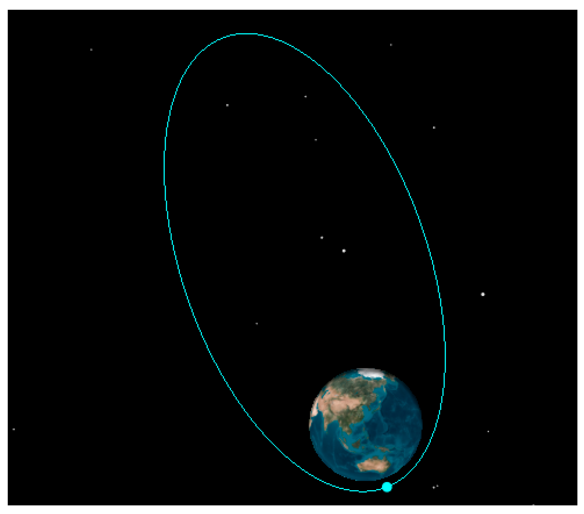
4.3. BDS-3+HEO Constellation

Although the hybrid constellation is applied in BDS and QZSS to improve the visibility in some specific areas, the visibility in polar regions is still unfavorable. This is because that, for the current GNSS constellations, when the station is at higher latitudes, the elevation of satellites that can be observed is lower. If satellites that can cover high latitude regions are included in the GNSS+ constellation, the geometric distribution for such regions will be improved. The HEO satellites, for example, the Russian Molniya satellites, are the kind of satellites that can fulfill this function [19]. These satellites have synchronous 12 h orbits of 500–40,000 km altitude that are inclined at an angle of 63.4° to the equator which can not only ensure an exceptional coverage of the Northern Hemisphere but also minimizes the impact of orbital perturbations caused by the earth’s oblateness. The HEO satellite’s parameters applied in this study are listed in

Table 5. Highly eccentric orbits (HEO) parameters.

Orbit Parameter	Nominal Value
Semi-major axis	42,165 km
Eccentricity	0.740969
Inclination	63.4°
Argument of perigee	270°
Center of longitude	118° E

and their ground track is continuously repeated as shown in Figure 6. The HEO in the 3D graphic view is displayed in Figure 7.

Five HEO satellites and BDS-3 satellites are combined to establish the BDS-3+HEO constellation. The primary constellation parameters are listed in

Table 6. Parameters of the BDS-3+HEO constellation.

Parameter	BDS-3+HEO
Orbit Type	MEO	IGSO	GEO	HEO
Nominal Number	24	3	3	5
Inclination	55°	55°	0°	63.4°
Altitude (km)	21,528	35,786	35,786	500–40,000
Period(s)	46,404	86,170.5	86,170.5	43,061

.

We evaluate the performance of the BDS-3+HEO constellation on a global scale, as illustrated in Figure 8.

The detailed improvement rates of introducing HEO satellites relative to BDS-3 at 30° N–90° N region are summarized in

Table 7. Improvement rates (%) of introducing HEO satellites relative to BDS-3 at 30° N–90° N region.

Average (Min–Max)
VisiNum	GDOP	PDOP	HDOP	VDOP	TDOP
38.76 (17.31–50.88)	15.70 (2.30–23.25)	16.65 (2.65–24.96)	10.35 (4.04–18.68)	16.65 (2.65–24.96)	11.52 (0–22.73)

. As can be seen from Figure 8 and Table 7, the DOPs and satellite visibility are modified favorably after using 5 HEO satellites. In the 30° N–90° N region, the satellite visibility is improved on average by 38.76%. In addition, all kinds of DOPs are improved. By introducing five HEO satellites to BDS-3, on average, values of the GDOP, PDOP, HDOP, VDOP, and TDOP are reduced by 15.70%, 16.65%, 10.35%, 16.65%, and 11.52% respectively. However, the correlation level between station height and receiver clock difference is still higher. As shown in Figure 8h, the correlation level in low latitude and the polar region is slightly higher. What is more, as revealed in Figure 8g and Figure 9, after applying HEO satellites, in some regions such as north polar and low latitude regions, positioning precision in longitude is better than in the latitude component. This may be since IGSO and HEO satellites mainly fly along the north-south direction, which would contribute to the DOP value in the longitude component mainly.

4.4. BDS-3+LEO+HEO Constellation

The augmentation of GNSS with LEO satellites is one of the most interesting trends in the future. We consider the addition of 288 LEO satellites in polar orbits which is mentioned in Li et al. [25] to form the BDS-3+LEO+HEO constellation. The primary constellation parameters are listed in

Table 8. Parameters of the BDS-3+ low earth orbit (LEO)+HEO constellation.

Parameter	BDS-3+LEO+HEO
Orbit Type	MEO	IGSO	GEO	LEO	HEO
Nominal Number	24	3	3	288	5
Inclination	55°	55°	0°	90°	63.4°
Altitude (km)	21,528	35,786	35,786	1000	500–40,000
Period(s)	46,404	86,170.5	86,170.5	6307	43,061

. These LEO orbits are distributed in 12 planes and orbit altitudes of 1000 km as shown in Figure 10 in the 3D graphic view. Using the EGAPM, the performance of the BDS-3+LEO+HEO constellation is analyzed. The results are plotted in Figure 11.

As can be seen in Figure 11, after introducing the LEO satellites, the DOPs have decreased significantly, which means that the geometric distribution has been improved. Since all LEO satellites are in polar orbits, a lot more satellites can be observed in high latitude regions than in the middle and low latitude areas (Figure 11a). Although hundreds of LEO satellites in polar orbits are introduced, the correlation between station height and receiver clock difference is still higher (Figure 11h). As for the positioning precision ratio between the longitude and latitude, illustrated in Figure 11g, Figure 9, and Figure 8g. We can find that LEO satellites mainly contribute to longitude component performance.

Table 9. Global average visible satellites and dilution of precision (DOP) values improving rates of BDS-3+HEO+LEO relative to BDS-3 and GPS.

Constellation	VisiNum	GDOP	HDOP	PDOP	TDOP	VDOP
BDS-3	197.81%	42.86%	43.59%	47.62%	49.32%	41.09%
GPS	183.99%	40.00%	41.33%	45.34%	46.38%	38.71%

reveals the average, minimal, and maximal improving rates of visible satellites and DOPs on a global scale. More satellites, with improving rate of 198% and 184%, respectively, for BDS-3 and GPS, can be observed. Besides, DOP values are about 40% lower than BDS-3 and GPS, which may improve the standard point positioning (SPP) accuracy and accelerate the precise point positioning (PPP) convergence speed.

5. Discussion

This article aims to provide a convenient way of assessing the global distribution of DOP and satellite visibility for the arbitrary navigation satellite constellation design. To do so, we replace the conventional point-by-point simulation of the constellation by statistical considerations of the probability of finding in certain viewing directions. We extend an earlier work of Wang et al. [15] and Wang et al. [16] to include non-circular orbits in analysis and present results for various sets of mixed-orbit constellations. Unfortunately, a disadvantage is also existing that EGAPM is not suitable to assess the ambiguity dilution of precision (ADOP), which can predict when ambiguity resolution can be expected to be successful [31,33,34,35]. Applying EGAPM, if a large number of grids or points can be viewed regarded as satellites and their ambiguities are estimated, the computation burden will be too heavy. What is worse, the calculation results of ADOP are not coincident with corresponding results calculated by GFZ precise ephemerides. However, in our next research, we will commit to finding a more ingenious way to solve this problem.

6. Conclusions

Hybrid constellations will be one of the development trends in the future; hence, it is necessary to develop a simple strategy to evaluate the performance of GNSS+ constellations before these satellites are launched. We extend the previous GAPM, which is only suitable for circular orbits. Furthermore, most calculations of satellite visibility and DOPs are based on real or complex simulated ephemerides. However, our strategy estimates satellite visibility and DOPs based on a few orbital parameters of one satellite constellation.

The features of the BDS-3 and GPS constellation were investigated. Satellite visibility of GPS is more balanced on a global scale than BDS-3. In contrast, for BDS-3, more satellites can be observed in the Asia-Pacific region and fewer satellites in the Western Hemisphere. VDOP is larger, especially in the polar regions for both BDS-3 and GPS. Furthermore, it is interesting to find that for the BDS-3 constellation, the precision in the longitude component is better in some low latitude and some polar regions, which are in contrast to GPS in these areas. Besides, the correlation level between station height and receiver clock difference is higher for both BDS-3 and GPS.

For QZO satellites, their orbit’s eccentricity is 0.075, and apogee is located above the Northern Hemisphere. Thus, these satellites stay a longer time above the Northern Hemisphere. Experiments show that when the BDS IGSO satellite is replaced by the QZO satellite, satellite visibility and GDOP are slightly better in the Northern Hemisphere but worse in the Southern Hemisphere relative to the BDS-3 constellation.

HEO satellites are introduced to improve satellite visibility in high latitude regions. The performance of the BDS-3+HEO constellation is assessed, and results show that the geometric distribution in the middle and high latitude regions is significantly improved. It is worth noting that VDOP is decreased by 16.65%, and satellite visibility improved by 38.76% on average in the 30° N–90° N region.

The performance of LEO satellites is also investigated, and the BDS-3+HEO+LEO constellation is analyzed. By introducing hundreds of LEO satellites, DOPs decreased greatly, 40% lower or so relative to the BDS-3 and GPS constellation on a global scale. In the meantime, it is interesting to find that the ratio of positioning precision between the longitude and the latitude component is strongly related to the direction of satellite travel. As LEO satellites are all at polar orbits, mainly flying along north-south direction and experiment results reveal that positioning accuracy is better in the longitude component in most regions.

The results and conclusion of this paper present a preliminary exploration for the design of the GNSS+ constellation and thus may benefit future GNSS development.

References

1. Xiao, W.; Liu, W.; Sun, G. Modernization milestone: BeiDou M2-S initial signal analysis. GPS Solut. 2016, 20, 125–133. [Google Scholar] [CrossRef]
2. Zhang, Y.; Kubo, N.; Chen, J.; Wang, J.; Wang, H. Initial positioning assessment of BDS new satellites and new signals. Remote Sens. 2019, 11, 1320. [Google Scholar] [CrossRef] [Green Version]
3. Montenbruck, O.; Steigenberger, P.; Hauschild, A. Multi-GNSS signal-in-space range error assessment—Methodology and results. Adv. Sp. Res. 2018, 61, 3020–3038. [Google Scholar] [CrossRef]
4. Wang, A.; Chen, J.; Zhang, Y.; Wang, J.; Wang, B. Performance evaluation of the CNAV broadcast ephemeris. J. Navig. 2019, 72, 1331–1344. [Google Scholar] [CrossRef]
5. Lv, Y.; Geng, T.; Zhao, Q.; Xie, X.; Zhou, R. Initial Assessment of BDS-3 preliminary system signal-in-space range error. GPS Solut. 2020, 24, 16. [Google Scholar] [CrossRef]
6. Wang, G.; de Jong, K.; Zhao, Q.; Hu, Z.; Guo, J. Multipath analysis of code measurements for BeiDou geostationary satellites. GPS Solut. 2015, 19, 129–139. [Google Scholar] [CrossRef]
7. Wang, M.; Wang, J.; Dong, D.; Li, H.; Han, L.; Chen, W. Comparison of three methods for estimating GPS multipath repeat time. Remote Sens. 2018, 10, 6. [Google Scholar] [CrossRef] [Green Version]
8. Hadas, T.; Kazmierski, K.; Sośnica, K. Performance of Galileo-only dual-frequency absolute positioning using the fully serviceable Galileo constellation. GPS Solut. 2019, 23, 108. [Google Scholar] [CrossRef] [Green Version]
9. Zhang, Z.; Li, B.; Nie, L.; Wei, C.; Jia, S.; Jiang, S. Initial assessment of BeiDou-3 Global navigation satellite system: Signal quality, RTK and PPP. GPS Solut. 2019, 23, 111. [Google Scholar] [CrossRef]
10. Mozo-García, Á.; Herráiz-Monseco, E.; Martín-Peiró, A.B.; Romay-Merino, M.M. Galileo constellation design. GPS Solut. 2001, 4, 9–15. [Google Scholar] [CrossRef]
11. Santerre, R. Impact of GPS satellite sky distribution. Manuscr. Geod. 1991, 16, 28–53. [Google Scholar]
12. Kihara, M.; Okada, T. A satellite selection method and accuracy for the global positioning system. Navigation 1984, 31, 8–20. [Google Scholar] [CrossRef]
13. Zhou, F.; Dong, D.; Ge, M.; Li, P.; Wickert, J.; Schuh, H. Simultaneous estimation of GLONASS pseudorange inter-frequency biases in precise point positioning using undifferenced and uncombined observations. GPS Solut. 2018, 22, 19. [Google Scholar] [CrossRef]
14. Yang, Y.; Li, J.; Wang, A.; Xu, J.; He, H.; Guo, H.; Shen, J.; Dai, X. Preliminary assessment of the navigation and positioning performance of BeiDou regional navigation satellite system. Sci. China Earth Sci. 2014, 57, 144–152. [Google Scholar] [CrossRef]
15. Wang, M.; Wang, J.; Dong, D.; Meng, L.; Chen, J.; Wang, A.; Cui, H. Performance of BDS-3: Satellite visibility and dilution of precision. GPS Solut. 2019, 23, 56. [Google Scholar] [CrossRef]
16. Wang, J.; Iz, B.; Lu, C. Dependency of GPS positioning precision on station location. GPS Solut. 2002, 6, 91–95. [Google Scholar] [CrossRef]
17. Chen, J.; Wang, A.; Zhang, Y.; Zhou, J.; Yu, C. BDS satellite-based augmentation service correction parameters and performance assessment. Remote Sens. 2020, 12, 766. [Google Scholar] [CrossRef] [Green Version]
18. Khon, V.C.; Mokhov, I.I.; Latif, M.; Semenov, V.A.; Park, W. Perspectives of northern sea route and northwest passage in the twenty-first century. Clim. Chang. 2010, 100, 757–768. [Google Scholar] [CrossRef]
19. Montenbruck, O.; Gill, E. Satellite Orbits; Springer: Berlin/Heidelberg, Germany, 2000; pp. 15–32. ISBN 78-3-540-67280-7. [Google Scholar] [CrossRef]
20. Yahya, M.H.; Kamarudin, M.N. Analysis of GPS visibility and satellite-receiver geometry over different latitudinal regions. In Proceedings of the International Symposium on Geoinformation (ISG 2008), Kuala Lumpur, Malaysia, 13–15 October 2008. [Google Scholar]
21. Chiang, K.-W.; Huang, Y.-S.; Tsai, M.-L.; Chen, K.-H. The perspective from Asia concerning the impact of Compass/Beidou-2 on future GNSS. Surv. Rev. 2010, 42, 3–19. [Google Scholar] [CrossRef]
22. Meng, X.; Roberts, G.W.; Dodson, A.H.; Cosser, E.; Barnes, J.; Rizos, C. Impact of GPS satellite and pseudolite geometry on structural deformation monitoring: Analytical and empirical studies. J. Geod. 2004, 77, 809–822. [Google Scholar] [CrossRef]
23. Chen, J. On Precise Orbit Determination of Low Earth Orbiters. Ph.D. Thesis, Tongji University, Shanghai, China, 2007. [Google Scholar]
24. Li, B.; Ge, H.; Ge, M.; Nie, L.; Shen, Y.; Schuh, H. LEO enhanced global navigation satellite system (LeGNSS) for real-time precise positioning services. Adv. Space Res. 2019, 63, 73–93. [Google Scholar] [CrossRef]
25. Li, X.; Ma, F.; Li, X.; Lv, H.; Bian, L.; Jiang, Z.; Zhang, X. LEO Constellation-augmented multi-GNSS for rapid PPP convergence. J. Geod. 2019, 93, 749–764. [Google Scholar] [CrossRef]
26. Li, X.; Lv, H.; Ma, F.; Li, X.; Liu, J.; Jiang, Z. GNSS RTK positioning augmented with large LEO constellation. Remote Sens. 2019, 11, 228. [Google Scholar] [CrossRef] [Green Version]
27. CSNO. BeiDou Navigation Satellite System Signal in Space Inter-Face Control Document—Open Service Signal B1I (Version 3.0); China Satellite Navigation Office: Beijing, China, 2019. [Google Scholar]
28. CSNO. Report on the Development of BeiDou Navigation Satellite System (Version 2.1); China Satellite Navigation Office: Beijing, China, 2012. [Google Scholar]
29. QZSS. Quasi-Zenith Satellite System Performance Standard (PS-QZSS-001). Cabinet Office, National Space Policy Secretariat. 2018. Available online: https://qzss.go.jp/en/technical/download/pdf/ps-is-qzss-001.pdf?t=1577867270694 (accessed on 5 November 2018).
30. Hofmann-Wellenhof, B.; Lichtenegger, H.; Wasle, E. GNSS—Global Naviagtion Satellite System; Springer: Vienna, Austria, 2008; pp. 322–341. ISBN 978-3-211-73012-62007. [Google Scholar]
31. Zaminpardaz, S.; Wang, K.; Teunissen, P.J.G. Australia-first high-precision positioning results with new Japanese QZSS regional satellite system. GPS Solut. 2018, 22, 101. [Google Scholar] [CrossRef] [Green Version]
32. Zhang, Y.; Kubo, N.; Chen, J.; Chu, F.; Wang, H.; Wang, J. Contribution of QZSS with four satellites to multi-GNSS long baseline RTK. J. Spat. Sci. 2020, 65, 41–60. [Google Scholar] [CrossRef]
33. Wang, K.; Teunissen, P.J.G.; El-Mowafy, A. The ADOP and PDOP: Two complementary diagnostics for GNSS positioning. J. Surv. Eng. 2020, 146, 04020008. [Google Scholar] [CrossRef] [Green Version]
34. Teunissen, P.J.G. A canonical theory for short GPS baselines. Part IV: Precision versus reliability. J. Geod. 1997, 71, 513–525. [Google Scholar] [CrossRef] [Green Version]
35. Odijk, D.; Teunissen, P.J.G. ADOP in Closed form for a hierarchy of multi-frequency single-baseline GNSS models. J. Geod. 2008, 82, 473–492. [Google Scholar] [CrossRef] [Green Version]
Figure 1. Distribution of observing probability for three third-generation BeiDou navigation satellite system (BDS-3) inclined geosynchronous orbit (IGSO) satellites.
Remotesensing 12 02560 g001
Figure 2. Distribution of observing probability for three Quasi-Zenith orbit (QZO) satellites.
Remotesensing 12 02560 g002
Figure 3. Estimation and reference value of the number of visible satellites for 32 Global Positioning System (GPS) satellites and the BDS-3+QZO constellation at all latitudes (−90° S–90° N) for the cutoff elevation angle (CEA) of 5°. (a) Estimation and reference value of the number of visible satellites for 32 GPS satellites; (b) Estimation and reference value of the numbers of visible satellites for BDS-3+QZO.
Remotesensing 12 02560 g003
Figure 4. Estimated DOPs (GDOP (geometric DOP), HDOP (horizontal DOP), PDOP (position DOP), TDOP (time DOP), and VDOP (vertical DOP) ), positioning precision in longitude versus latitude, and correlation between station height and receiver clock difference of the BDS-3 and GPS constellation with 5° CEA. (a) Number of visible satellites BDS-3; (b) Number of visible satellites GPS; (c) GDOP of BDS-3; (d) GDOP of GPS; (e) HDOP of BDS-3; (f) HDOP of GPS; (g) PDOP of BDS-3; (h) PDOP of GPS; (i) TDOP of BDS-3; (j) TDOP of GPS; (k) VDOP of BDS-3; (l) VDOP of GPS; (m) The ratio of positioning precision between the longitude component and the latitude component of BDS-3; (n) The ratio of positioning precision between the longitude component and the latitude component of GPS; (o) Correlation level between station height and receiver clock difference of BDS-3; (p) Correlation level between station height and receiver clock difference of GPS.
Remotesensing 12 02560 g004aRemotesensing 12 02560 g004b
Figure 5. The performance improving rates (%) of BDS-3+QZO relative to the BDS-3 constellation in area of 90° S–90° N and 50° E–170° E. (a) Satellites visibility improving rates of BDS-3+QZO relative to BDS-3; (b) GDOP improving rates of BDS-3+QZO relative to BDS-3
Remotesensing 12 02560 g005
Figure 6. Ground track of highly eccentric orbits (HEO) satellites.
Remotesensing 12 02560 g006
Figure 7. HEO in the three-dimensional (3D) graphic view.
Remotesensing 12 02560 g007
Figure 8. Estimated DOPs, positioning precision in longitude versus latitude, and the correlation between station height and receiver clock difference of the BDS-3+HEO constellation. (a) Number of visible satellites; (b) GDOP; (c) HDOP; (d) PDOP; (e) TDOP; (f) VDOP; (g) The ratio of positioning precision between the longitude component and the latitude component; (h) Correlation level between station height and receiver clock difference.
Remotesensing 12 02560 g008
Figure 9. The ratio of positioning precision between the longitude component and the component latitude for BDS-3.
Remotesensing 12 02560 g009
Figure 10. Low earth orbit (LEO) satellites in the 3D graphic view.
Remotesensing 12 02560 g010
Figure 11. Estimated DOPs, positioning precision in longitude versus in latitude, and the correlation between station height and receiver clock difference of the BDS-3+LEO+HEO constellation with 5° CEA. (a) Number of visible satellites; (b) GDOP; (c) HDOP; (d) PDOP; (e) TDOP; (f) VDOP; (g) The ratio of positioning precision between the longitude component and the latitude component; (h) The correlation level between station height and receiver clock difference.
Remotesensing 12 02560 g011