Article

Fusion of Multiple Gridded Biomass Datasets for Generating a Global Forest Aboveground Biomass Map

1
Beijing Engineering Research Center of Industrial Spectrum Imaging, School of Automation and Electrical Engineering, University of Science and Technology Beijing, Beijing 100083, China
2
Department of Geographical Sciences, University of Maryland, College Park, MD 20740, USA
*
Author to whom correspondence should be addressed.
Remote Sens. 2020, 12(16), 2559; https://doi.org/10.3390/rs12162559
Submission received: 9 June 2020 / Revised: 19 July 2020 / Accepted: 28 July 2020 / Published: 9 August 2020

Abstract

:
Many advanced satellite estimation methods have been developed, but global forest aboveground biomass (AGB) products remain largely uncertain. In this study, we explored data fusion techniques to generate a global forest AGB map for the 2000s at 0.01-degree resolution with improved accuracy by integrating ten existing local or global maps. The error removal and simple averaging algorithm, which is efficient and makes no assumption about the data and associated errors, was proposed to integrate these ten forest AGB maps. We first compiled the global reference AGB from in situ measurements and high-resolution AGB data that were originally derived from field data and airborne lidar data and determined the errors of each forest AGB map at the pixels with corresponding reference AGB values. Based on the errors determined from reference AGB data, the pixel-by-pixel errors associated with each of the ten AGB datasets were estimated from multiple predictors (e.g., leaf area index, forest canopy height, forest cover, land surface elevation, slope, temperature, and precipitation) using the random forest algorithm. The estimated pixel-by-pixel errors were then removed from the corresponding forest AGB datasets, and finally, global forest AGB maps were generated by combining the calibrated existing forest AGB datasets using the simple averaging algorithm. Cross-validation using reference AGB data showed that the accuracy of the fused global forest AGB map had an R-squared of 0.61 and a root mean square error (RMSE) of 53.68 Mg/ha, which is better than the reported accuracies (R-squared of 0.56 and RMSE larger than 80 Mg/ha) in the literature. Intercomparison with previous studies also suggested that the fused AGB estimates were much closer to the reference AGB values. This study attempted to integrate existing forest AGB datasets for generating a global forest AGB map with better accuracy and moved one step forward for our understanding of the global terrestrial carbon cycle by providing improved benchmarks of global forest carbon stocks.

1. Introduction

Forest aboveground biomass (AGB) is considered an essential climate variable and plays an important role in the climate system and the global carbon cycle [1]. Accurate estimation of forest AGB and its dynamics have been gaining widespread attention from the research community. Many scholars have attempted to map the spatial distribution of forest AGB across large regions from satellite observations using various algorithms, and a great number of AGB maps have thus been generated from local to global scales, with a spatial resolution mainly ranging from 250 m to 1 km [2,3,4]. For some specific regions, high-resolution AGB maps (e.g., 30 m) are also available [5,6].
On the global scale, Ruesch and Gibbs [7] provided the first spatially explicit estimate of vegetation biomass and carbon stocks at a 1-km resolution for the year 2000. They compiled a total of 124 carbon zones or regions with unique carbon stock values using the IPCC (International Panel on Climate Change) Tier-1 method and then mapped these unique carbon zones with spatial datasets, including land cover maps, ecoregions zones, and forest age, to generate the gridded carbon stock dataset. However, field data were not used in the generation or validation of the biomass dataset, and little is known about the uncertainties of the global carbon stock dataset. Following this study, Hengeveld et al. [8] provided global forest biomass at 1° spatial resolution with five-year intervals from 1950 to 2010 with forest area and growing stock data. Kindermann et al. [9] produced a global forest biomass dataset at 0.5° spatial resolution for the year 2005 based on the forest resources assessment (FRA) biomass and the assumed linear relationships between net primary production and biomass and between human activity and biomass. Liu et al. [10] derived global forest biomass carbon estimates at 0.25° spatial resolution from 1993 to 2012 from the empirical relationship between the Saatchi et al. [11] AGB map and the vegetation optical depth data that were estimated from passive microwave data. However, due to the lack of field data in these studies and the coarse spatial resolution of generated biomass maps, it is difficult to evaluate the accuracies of these global biomass datasets. Recently, some studies have adopted more advanced approaches for generating global forest AGB maps by integrating field data with multiple satellite datasets and ancillary data using machine learning algorithms. For example, Hu et al. [12] mapped the global forest AGB at 1 km resolution for the year 2004 through the integration of field inventory data, the Geoscience Laser Altimeter System (GLAS) data, optical imagery, climate surfaces, and topographic data using random forests (RF) model. Validation results with field data showed that the AGB map achieved accuracy with R2 of 0.56 and RMSE of 87.53 Mg/ha. Yang et al. [13] presented a global forest AGB map at a 1 km resolution for 2005 by combining field data with multiple satellite products, including leaf area index (LAI), gross primary production, canopy height map, vegetation continuous fields using the gradient boosting regression tree algorithm. Validation results from 20% independent samples, which were compiled from field data and regional biomass maps, showed the accuracy of generated forest AGB map had an R2 of 0.90 and RMSE of 35.87 Mg/ha. Despite these efforts to map forest AGB, substantial inconsistencies and uncertainties remain in existing forest AGB maps [14]. Different studies have produced quite diverse biomass maps in terms of both the magnitude and spatial distributions due to the uncertainties in the allometric equations used to calculate field biomass and the usage of different satellite data and mapping algorithms to estimate regional biomass [15,16]. To improve the situation, some recent studies have proposed reducing relevant uncertainties by comprehensively compiling field reference datasets [17], developing more advanced machine learning algorithms [18], and using novel remote sensing techniques (e.g., the European Space Agency P-band radar data and the Global Ecosystem Dynamics Investigation Lidar data) [19,20]. An alternative and promising method for improving the accuracy of AGB mapping is postprocessing the existing AGB maps using data integration or fusion techniques. Currently, a large number of forest AGB maps have been generated from multisource data using diverse algorithms [14], which offers the possibility of improving the accuracy of AGB mapping by combining this complementary information and advantages of each individual AGB map using data integration algorithms.
Data integration or data fusion is not novel in remote sensing fields. Previous studies have integrated multiple high-level satellite data products to estimate parameters with higher accuracy in geoscience [21,22]. For example, Chatterjee et al. [23] applied a simple geostatistical data fusion approach to merge multiple aerosol optical thickness (AOT) datasets and obtained an optimal fused AOT dataset. To solve the computational bottleneck that occurs when geostatistical data fusion methods are used for massive remote sensing datasets, Nguyen et al. [24] employed the spatial statistical data fusion approach in which the spatial covariance term was expressed by spatial basis functions and Gaussian random variables to integrate multiple AOT datasets. Wang and Liang [25] used the empirical orthogonal function (EOF)-based data integration method to estimate the leaf area index (LAI) from multiple high-level satellite data products and achieved significantly improved results compared with each of the original products. Compared with geostatistical approaches, the EOF-based algorithm is easy to implement and does not require a precalculated covariance model and estimation error matrix. In addition, studies on integrating satellite-derived products have included the multiresolution tree (MRT) method to fuse multiple land surface broadband albedo products, land surface emissivity, and the fraction of absorbed photosynthetically active radiation by green vegetation [26,27,28], the Bayesian maximum entropy method to fuse multiple-satellite AOD products and sea surface temperature products [29,30], and the geographically weighted regression model to integrate different global land cover maps and forest cover products [31,32].
However, in the field of forest AGB mapping, integrating available forest AGB maps to generate more accurate results has been largely ignored. Currently, few studies have attempted to combine existing forest AGB maps for a more accurate estimation of forest AGB. Ge et al. [33] first combined three source biomass maps covering East Africa with reference datasets using the weighted averaging approach and obtained more accurate biomass maps than each of the individual source biomass maps. Following this study, Avitabile et al. [34] fused pantropical forest biomass maps produced by Saatchi et al. [11] and Baccini et al. [4] using bias removal and the weighted linear averaging method and improved the estimation of forest AGB across pantropical regions. Here, we aimed to make the best use of existing AGB maps from local to global scales to generate a global forest biomass map with greater accuracy than existing AGB maps.
As noted, many algorithms have been proposed to integrate satellite data products. However, most of them are based on the assumption that satellite products have white noise that follows a normal distribution [21], which is rarely satisfied by regional and global forest AGB data. Additionally, the complex structures of these fusion algorithms affect the computational efficiency for calculating the weightings of individual datasets, which limits their application on a large scale [35]. Instead of only considering the effectiveness of the fused results, linear combination methods can achieve good results in effectiveness and efficiency and thus have received much attention in information retrieval, especially in the big data environment [36]. The linear combination method can be very flexible since different weights can be easily assigned to different data products. According to the weights used in the combination, diverse linear combination methods have been developed, but which weighting schema is good remains an open question [37]. In this study, to reduce the complexity of the fusion algorithm that was used to generate a more accurate global forest AGB map, we proposed a linear combination algorithm that first removes the corresponding errors from gridded forest AGB datasets and then simply averages the calibrated forest AGB data for the fusion of multiple forest AGB datasets. The objectives of this study were thus to (1) improve the accuracy of biomass estimates by integrating multiple forest AGB maps with the proposed error removal and simple averaging algorithm and (2) generate an accurate forest AGB map at a global scale.

2. Materials and Methods

2.1. Regional and Global Source AGB Maps

We collected existing regional and global forest AGB maps that were derived from satellite observations. If more than one version of a gridded AGB map was available, the improved version with higher accuracy was used for the fusion algorithm in this study. Ten forest AGB maps were finally selected and served as input layers for global forest AGB mapping (hereafter referred to as source AGB maps). The 10 source AGB maps should represent state-of-the-art AGB estimates covering different regions. To facilitate description, they were named producers plus biomass (e.g., Avitabile biomass) if they did not have a specified name. The spatial and temporal coverage, spatial resolutions, and mapping algorithms of 10 source AGB maps are listed in Table 1, and more details about these datasets can be found in the corresponding references.
GLC2000, Global Land Cover 2000; MODIS, Moderate Resolution Imaging Spectroradiometer; EOSD, Earth Observation for Sustainable Development of Forests; ASAR, Advanced Synthetic Aperture Radar; NLCD, National Land Cover Dataset; PALS, Portable Airborne Laser System; GEZ, Global Ecological Zones; NDVI, Normalized Difference Vegetation Index; SRTM, Shuttle Radar Topographic Mission; DEM, Digital Elevation Model; InSAR, Interferometric Synthetic Aperture Radar.
The pantropical Avitabile biomass map was derived from existing AGB datasets published by Saatchi et al. [11] and Baccini et al. [4] and had higher accuracy [34]. Due to the incorporation of Avitabile biomass map, Saatchi biomass and Baccini biomass were not considered as source AGB maps in this study. The Avitabile biomass map was provided in a geographic projection (WGS-84) at 0.00833 degrees (approximately 1 km) resolution and resampled to 0.01°.
Thurner et al. [3] provided forest carbon density at 0.01° resolution in Northern Hemisphere boreal and temperate regions (30°–80°N) based on a growing stock volume product retrieved from synthetic aperture radar, wood density, and biomass compartment data. They used a carbon fraction of 0.488 for broadleaf tree species and 0.508 for needleleaf tree species to calculate carbon density. We adopted a common factor of 2.0 to convert the carbon density (Mg C/ha) to AGB (Mg/ha) since forest types might be a mixture of several forest types at the pixel level, and it is difficult to separate them. Similar to Thurner et al. [3], the maps generated by Wilson et al. [39] provided aboveground carbon density (Mg·C/ha), and a carbon concentration of 0.5 gC·g−1 was used to convert carbon density to AGB (Mg/ha).
Neigh biomass and Margolis biomass were generated using similar methods that tied ground plot AGB to airborne profiling lidar metrics as well as GLAS data and had a spatial resolution of 500 m [38,43]. The preprocessing of both datasets included reprojection to the WGS84 coordinate system and aggregation to the 0.01° resolution by computing the mean value of the pixels whose center was located within each 0.01° cell.
Additionally, Blackard biomass, Wilson biomass, NBCD2000, and Su biomass were not expressed in the geographical coordinate system and were first reprojected from their original projection type to the geographical coordinate system with WGS84 datum using the nearest-neighbor resampling method. Source AGB maps with spatial resolutions finer than 0.01°, such as Blackard biomass and NBCD2000, were aggregated to the 0.01° resolution.

2.2. Reference AGB Datasets

The reference AGB data were used to calibrate source AGB maps and validate the accuracy of the generated global forest AGB map using the data fusion technique. Reference AGB was obtained by compiling field measurements and high-resolution biomass datasets that were originally derived from field data and lidar data [44]. Field biomass measurements were compiled from plot-level AGB that were acquired on or after the year 2000 from the published literature and online databases. These plots were mainly located in the mature or primary forest with minimal human disturbances. For each plot, the coordinate information, plot name, plot code, plot size, forest status (e.g., old-growth or regrowth), sampling years, as well as the corresponding forest AGB were recorded. Plot-level AGB was estimated using allometric equations developed for a specific region or a specific type of forest. Only trees above a defined diameter at breast height (1.3 m above the ground) larger than or equal to 10 cm were considered to computing plot-level AGB [45,46,47,48]. For field plots that provided carbon density rather than AGB, a carbon concentration of 0.5 gC·g−1 was used to calculate AGB in the unit of Mg/ha. To ensure the representativeness of in-situ plot measurements to the forest conditions of corresponding locations and reduce the potential error in data geolocation, the collected plots less than 0.05 ha in size were filtered out [49,50]. A total of 5885 field plots from 25 sources were selected and aggregated into 2199 reference AGB cells with 0.01° resolution (Table 2).
High-resolution biomass datasets were used to generate reference AGB data because of their relatively high accuracies. Generally, field plots had a size of approximately 0.25~1.0 ha, corresponding to a pixel size of approximately 50~100 m; therefore, we only considered gridded biomass maps with spatial resolutions finer than 100 m to ensure that field datasets and high-resolution biomass datasets could match well at the spatial scale. Six datasets were selected to derive reference AGB data, including the Cook biomass map at four forested sites in the US: Garcia River Tract in California, Anne Arundel and Howard Counties in Maryland, Parker Tract in North Carolina, and Hubbard Brook Experimental Forest in New Hampshire, for the nominal year of 2011 at 20–50-m resolution [70]; the Babcock biomass map at 13-m spatial resolution in the Penobscot Experimental Forest (PEF) in Bradley, Maine, for the year 2012 [71]; the Dubayah biomass map at a 30-m spatial resolution for Maryland for the nominal year 2011 [72]; the Dubayah map for Sonoma County, California, for the nominal year 2013 [73]; the Labberière River biomass data at two sites in French Guiana and four areas in Gabon [58]; the Fatoyinbo biomass map at a 1-m spatial resolution for a mangrove forest in the Zamamamamé Delta Mombita Mozaque forest [74]. Consistent with the preprocessing of source AGB maps, the preprocessing of high-resolution biomass maps included reprojection to the geographical coordinate system and aggregation to the 0.01° scale. For the biomass maps that provided carbon density values instead of AGB, the common factor 2.0 was used to convert carbon density to AGB.
We combined the aggregated field reference data and high-resolution reference biomass datasets and generated a global reference AGB dataset. Since the mismatches in spatial scales between field plots and pixels of satellite products may lead to uncertainties of forest AGB mapping, particularly when forest AGB showed strong local spatial variation [75], we assessed the spatial variation in reference AGB datasets using the coefficient of variation (CV) of tree cover data from Hansen et al. [76] within each 0.01° pixel and removed the reference AGB data with a CV of tree cover larger than 1.0, leaving 13,597 pixels (Figure 1).

2.3. Data Fusion Framework

Based on the generated reference AGB data in Section 2.2, source AGB maps were integrated using the linear combination method. The integration of multiple-satellite data products was essentially a weighted combination of multiple datasets. Estimating forest AGB from multiple source AGB maps can be expressed as:
Y ( k ) = i = 1 N w i ( k ) X i ( k )
i = 1 N w i = 1
where k represents the forest pixel, Y(k) is the estimated biomass of pixel k, N is the number of source AGB maps with biomass values for pixel k, Xi is the AGB value of the i-th source map, and wi(k) is the weight that was set for the i-th source AGB map at pixel k. For any pixel, the sum of all the weights of the source AGB maps is equal to 1.
Since the calculation of weights greatly affects the estimated AGB, we explored several algorithms, including the adaptive-weighted average algorithm that computes the weights of each source AGB map by its prediction performance [77] and the skill and independence weighted average algorithm, which can account for both the performances of source AGB maps and independences among these AGB maps [78], and found that these weighted average algorithms could not provide accurate estimates of forest AGB. Therefore, we proposed the error removal and simple averaging method for the fusion of ten source AGB maps.
Using the error removal and simple averaging algorithm, estimated pixel-level AGB was derived as follows:
Y i ( k ) = 1 N i = 1 N ( X i ( k ) E i ( k ) )
where k represents the forest pixel, Y(k) is the estimated biomass of pixel k, N is the number of source AGB maps with biomass values at pixel k, X is the observed biomass of the i-th source AGB map, and Ei(s) is the error of the i-th source biomass map at pixel k.
According to Equation (3), estimating AGB from multiple source maps consisted of the following steps: (1) determine the pixel-level errors of each source AGB map, (2) calibrate the source AGB by removing the corresponding pixel-level errors, and (3) average the calibrated source AGB maps with equal weights. The core of the proposed error removal and the simple average algorithm was to obtain pixel-level errors associated with each source AGB map. Once we modeled the errors of each source AGB map, estimated AGB through the fusion of source AGB maps could be obtained using Equation (3).

2.4. Estimating Pixel-Level Errors of Source AGB Maps

The accuracies or performances of a source AGB map were not uniformly distributed across its whole coverage, and in addition, source AGB maps were not accompanied by a pixel-level error or uncertainty map. It was thus necessary to estimate the pixel-level errors of AGB data. For each source AGB map, pixel-level errors of AGB values corresponding to reference AGB data points were obtained from the differences between extracted AGB from the source AGB map and coincident reference AGB data and used as the training samples for estimating pixel-level errors of AGB. Pixel-level errors of source AGB maps were obtained by extrapolating the dispersed observational errors into the same spatial extent as the source AGB maps. In this study, we implemented extrapolation with the random forest regression tree algorithm. Predictor variables were the leaf area index (LAI), forest canopy height, forest cover, elevation and slope, and temperature and precipitation, which were correlated with forest AGB [34].
The Global Land Surface Satellites (GLASS) LAI product, with a temporal resolution of eight days and a spatial resolution of 1 km from 2000 to 2010, was used [79,80]. To reduce the noise in the LAI time series and minimize the impacts of LAI seasonality on biomass estimates, we aggregated the 8-day LAI to the monthly scale and extracted the maximum monthly LAI within one year as the maximum annual LAI. The LAI used in the error modeling was the average of the maximum annual LAI values from 2001–2010. The global forest canopy height map was provided by Simard et al. [81], with a 1-km spatial resolution. The global forest cover map at 30-m spatial resolution generated by Hansen et al. [76] was aggregated to 0.01 degrees and used as one of the covariates of errors. It also served as the base map of the global tree cover. Forests and shrubs with a tree cover of no less than 10% were considered forest pixels, and other pixels were masked [82]. Additionally, the land surface elevation and slope information derived from the Global Multiresolution Terrain Elevation Data (GMTED) 2010 dataset at 7.5 arc-second resolution [83], as well as the average monthly temperature and precipitation data at 30-s resolution download from WorldClim (http://worldclim.org/version2) [84], were included in the modeling of errors associated with each source AGB map. For consistency with AGB datasets, predictor variables, including LAI, forest canopy height, forest cover, elevation and slope, and climate data, were all reprojected to the WGS 84 geographical system and resampled to 0.01 degrees.

2.5. Validation and Intercomparison

Ten-fold cross-validation was performed to evaluate the accuracy of estimated forest AGB from multiple source AGB maps using the error removal and simple averaging algorithm. Evaluation metrics were the correlation of determination (R2), bias, and RMSE.
Intercomparison was also performed to indirectly assess the accuracy of our estimated results relative to global forest AGB maps from published studies, with AGB maps provided by Kindermann et al. [9], Liu et al. [10], Hu et al. [12], and Yang et al. [13]. Liu et al. [10] provided forest carbon estimates from 1993 to 2012 at a 0.25° resolution. We converted the carbon to biomass using the common factor and took the average AGB from 2001 to 2010 as the Liu biomass map used in the comparison. The Liu biomass map and the Kindermann et al. [9] AGB data for 2005 at a half-degree resolution had a spatial resolution coarser than 0.01° and were resampled to 0.01° for consistency with other global forest AGB maps.
We extracted the estimated AGB from four previous studies and fused the AGB of this study for the reference AGB pixels and assessed how closely the five global forest AGB data matched the reference AGB data. Their similarities with reference AGB data were quantified in terms of the correlation coefficients, standard deviation, and centered root-mean-square difference (RMSD) and graphically described by the Taylor diagram [85].
Additionally, we obtained the different AGB maps by subtracting each of the four global forest AGB maps from the fused AGB. Statistical analysis of AGB differences for different continents and frequency distributions of each global AGB map for different forest types were conducted. The forest types were separated according to the MODIS land cover type product (MCD12Q1, version 6) for 2005 and the International Geosphere-Biosphere Program legend [86]. Consistent with other global forest AGB data, the 500-m resolution data were first reprojected to the geographical coordinate system using the nearest-neighbor resampling method and then aggregated to the 0.01-degree resolution by selecting the most dominant land cover type within the extent of each 0.01-degree pixel. We extracted the AGB values with a corresponding tree cover of no less than 10% and forest types, including deciduous broadleaf forests (DBF), deciduous needleleaf forests (DNF), evergreen needleleaf forests (ENF), evergreen broadleaf forests (EBF), mixed forests (MF), open shrublands (OSH), closed shrublands (CSH), woody savannas (WSA), and savannas (SAV), and performed statistical analysis of the number of pixels within 20 Mg/ha bins. Since different definitions of forests were used in the generation of these forest AGB maps, all the statistical analyses were carried out on the pixels that were considered forests by the AGB datasets used in a comparison.

3. Results

3.1. Modeled Errors Associated with Source AGB Maps

Pixel-level errors associated with each source AGB map were modeled using the RF algorithms, and the results showed that the modeled errors were close to the observation errors, which were calculated from the difference between the reference AGB data and the corresponding gridded AGB extracted from the source map (Figure 2). The correlation coefficients between modeled error and observation error at reference AGB data points ranged from 0.76 for Su biomass to 0.90 for Hu biomass and Wilson biomass, while RMSEs of predicted errors in source AGB maps ranged from 26.48 Mg/ha to 79.59 Mg/ha. Three source AGB maps had RMSEs of less than 30 Mg/ha, four source datasets had RMSEs of 30~40 Mg/ha, and for the three remaining source AGB maps, including the Su biomass, Barredo biomass, and Avitabile biomass, the differences between observation errors and modeled errors at the reference AGB data points were relatively large. Nevertheless, the pixel-level errors in the majority pixels of each source AGB map were modeled accurately, very close to the observation errors, which also suggested the efficiency of our approach in estimating errors of source AGB maps (Figure 2).

3.2. Spatial Patterns of the Fused Global Forest AGB Map for the 2000s

Based on the pixel-by-pixel errors of each source AGB map, source AGB maps were calibrated and then averaged to generate the global forest AGB map for the 2000s (Figure 3). The results showed that tropical forests stocked the most carbon in the aboveground per hectare [9,12,87]. When aggregated to the country level, New Zealand, French Guiana, Equatorial Guinea, Gabon, Suriname, Guyana, Brunei Darussalam, and Congo were found to have the highest forest AGB, with corresponding forest area-weighted averages of AGBs higher than 300 Mg/ha. At the continental scale, the AGB of Oceania and South America was higher than those of other continents. Europe and Asia had the lowest forest AGB but exhibited different spatial patterns. In Europe, nearly all countries had low biomass densities, whereas, in Asia, there were large discrepancies in forest biomass among different countries.

3.3. Validation Results

Cross-validation results showed that the generated forest AGB map achieved a good overall accuracy, which had an R-squared of 0.61, RMSE of 53.68 Mg/ha, RMSE% of 30.28%, and bias of 3.15 Mg/ha globally (Figure 4). To the best of our knowledge, this accuracy is the best among studies on estimating forest AGB on a large scale. Another study that used satellite data and the RF algorithm to predict the forest AGB had an R-squared of 0.56 and RMSE of 87.53 Mg/ha on a global scale [12].

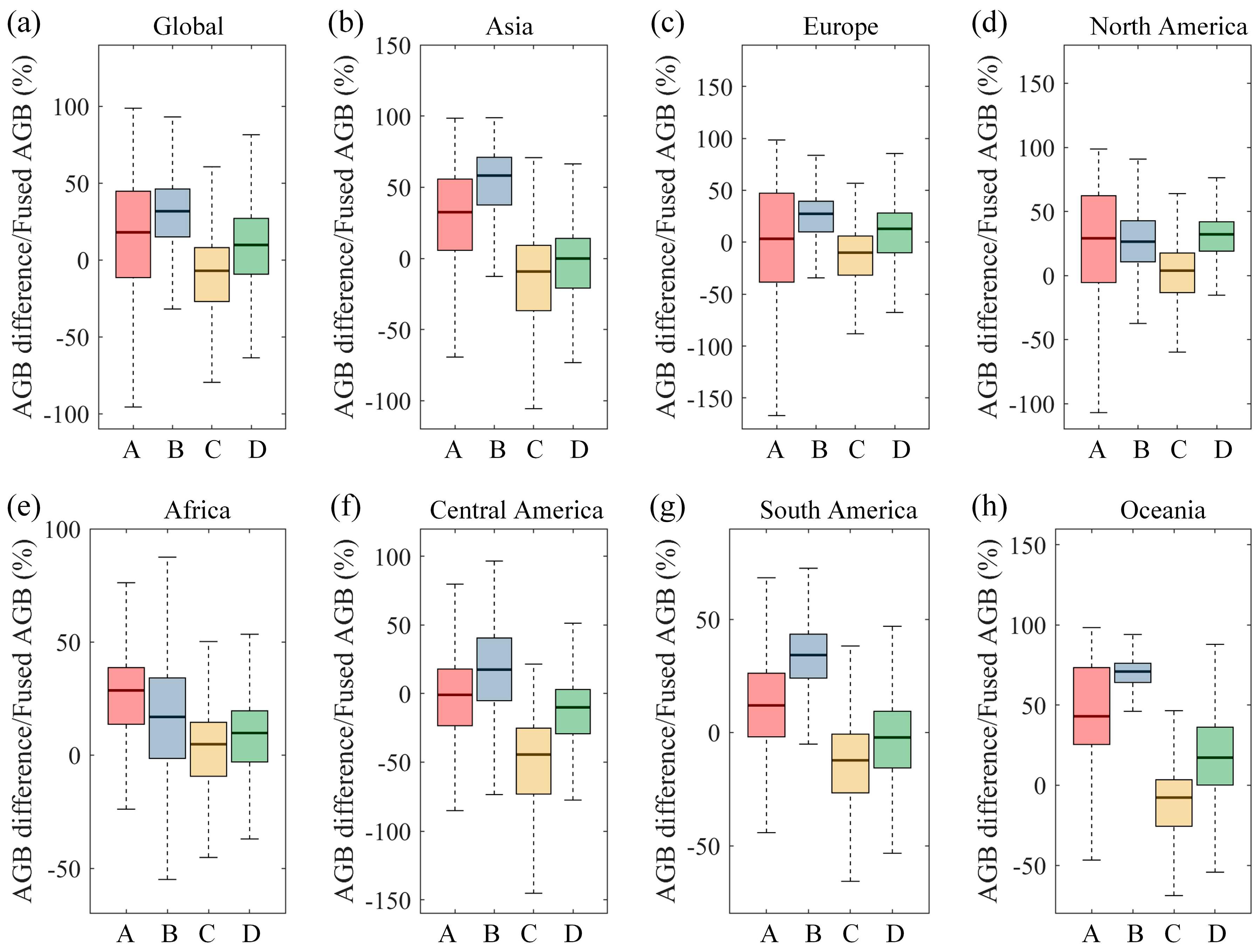
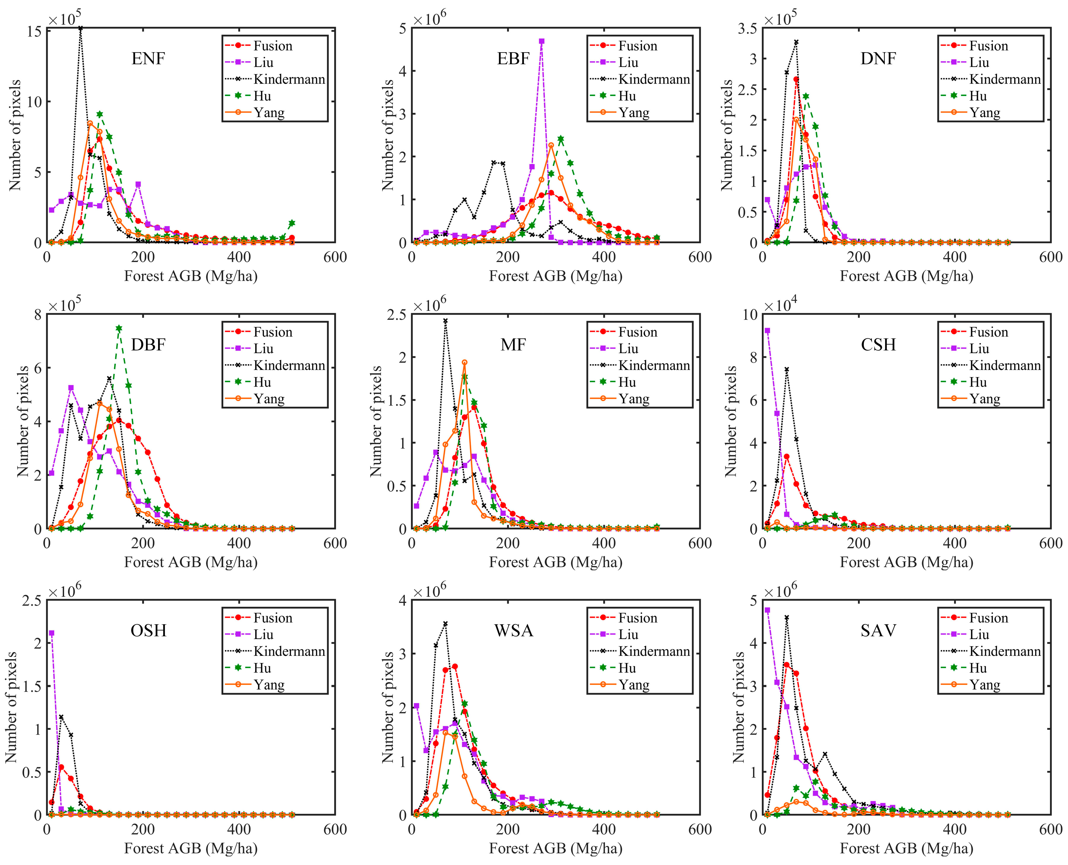
3.4. Intercomparison Results

Compared with global AGB maps from other studies, the forest AGB map generated by the fusion of source AGB maps (fused AGB) was closer to the reference AGB (Figure 5). Estimated AGB from Yang et al. [13] and Hu et al. [12] for the reference AGB pixels was similar in terms of correlation, standard deviation, and RMSD. AGB estimated by Liu et al. [10], Yang et al. [13], and Hu et al. [12] had similar standard deviations, but their correlations with reference AGB were slightly different. AGB estimated by Kindermann et al. [9] was quite different from other studies; it had the least standard deviation and correlation and the largest RMSD.
The spatial distribution of AGB differences between fused AGB and global AGB maps from other studies also showed substantial discrepancies in AGB estimation among different studies on a global scale (Figure 6). The fused AGB tended to be higher than the Liu AGB and Kindermann AGB for most forests in the world (Figure 6 and Figure 7) but slightly lower than the Hu AGB map at a global scale, which was probably caused by the extremely low fused AGB in Europe and Central and South America (Figure 7).
At the continental scale, the differences in five global forest AGB maps were not substantial in Europe and North America as in Oceania, Africa, Asia, and South America, consistent with published studies that emphasized the uncertainties of estimated AGB in tropical regions [4,88]. Since boreal forests have lower AGB than tropical forests, it is not appropriate to directly compare the uncertainties in estimated AGB for different regions. The intercomparison results of relative AGB differences showed that larger discrepancies in estimated AGB among different datasets existed for forests in Europe and North America, while the relative AGB differences in South America and Africa mostly ranged within ±50% (Figure 8). This indicated the strong necessity to improve the accuracy of AGB estimates in boreal forests, which is largely ignored in previous studies.
Comparing the frequency distributions of five global forest AGB datasets, we found that the frequency of fused AGB for all forest types except CSH had one peak, and the number of pixels with corresponding AGB values within the peak bins was small, suggesting that fused AGB had dispersed distributions compared with other datasets within each forest type (Figure 9). The Kindermann AGB data had quite different distributions from the other datasets, particularly in ENF, EBF, DNF, DBF, MF, and CSH. All the datasets except Kindermann revealed higher AGB in EBF than those in other forest types. DBF also had high AGB values, while DNF had lower AGB, distributed within a narrower range. Large discrepancies in the frequency distribution of Liu AGB with other datasets were also found in all forest types except WSA and SAV. In CSH, OSH, WSA, and SAV, this study provided lower AGB with more reasonable distributions than other datasets.

4. Discussions

4.1. Uncertainty Analysis of Global Forest AGB Mapping

The generated global forest AGB map was derived by merging ten source AGB maps using the error removal and simple averaging method. Uncertainties of this fused AGB map thus mainly come from the uncertainties of pixel-level errors of source AGB maps. If the errors of source AGB maps can be estimated accurately, the derived forest AGB map will have a high level of confidence. Although this study provided more accurate AGB estimates than published datasets globally, uncertainties are still large in some regions, partly attributed to the remotely sensed datasets used. The primary datasets were from optical sensors, which were responsive to canopy cover, rather than vertical structure. This could affect the accuracy of modeled errors of source AGB maps. Predictors that describe the vertical structure of forests should be included to improve the accuracy of modeled errors and further AGB estimates in future studies.
In this study, the accuracy of the modeled errors had R-squared values ranging from 0.58 to 0.81 and RMSE values ranging from 26.48 Mg/ha to 79.59 Mg/ha. Cross-validation results suggested that estimated global forest AGB achieved accuracy with an R-squared of 0.61 and RMSE of 53.68 Mg/ha, located within the accuracy of modeled errors of source biomass maps, which was probably because the discrepancies between real observation errors and the corresponding predicted errors accounted for the majority of uncertainties in forest AGB estimation. The results of this study indicated that accurate quantification or knowledge of uncertainties was not only important for understanding the uncertainty of the datasets and facilitating their application in related fields but also indispensable for improving the accuracy of estimated forest AGB.
Previous studies have quantified the pixel-level errors or uncertainties of biomass estimates mainly by the error propagation approach, calculating the uncertainties due to model algorithms, datasets used, the choice of allometric equations, and the mismatch of field data and remotely sensed data [89,90,91]. However, it is difficult to measure all the uncertainties in the AGB estimation since the influencing factors are so complex, and nearly all the studies have quantified only parts of the uncertainties in the AGB estimation. This study provided a new perspective to describe uncertainties without distinguishing the sources of uncertainties, which can help in understanding and quantifying uncertainties in forest AGB estimation in future studies.

4.2. Strength and Limitation of the Error Removal and Simple Averaging Method

The true AGB value can be mathematically described as the sum of observed or estimated AGB and the associated errors. If we can infer the errors associated with the estimated forest AGB, the true or actual forest AGB will be known. Therefore, to generate an accurate global forest AGB map, it is essential to quantify the pixel-level errors of source AGB maps accurately. Since it is difficult to quantify the errors or uncertainties in AGB estimates, the RF algorithm was used to model the pixel-level errors of each source AGB map in this study. The results showed that the modeled errors were close to the observational errors of the source biomass maps, which were obtained by comparison with reference AGB data. Different from most studies that use RF algorithms to estimate forest AGB with ancillary datasets, we used similar methods to estimate errors of AGB maps rather than AGB [92,93]. The underlying principle is that errors of estimation are often negatively correlated with the AGB values, partly due to the underestimation of AGB at low values and overestimation at high values caused by datasets and empirical modeling methods used, as demonstrated in previous studies [68]. Through estimating errors of source biomass maps and further calibrating these AGB maps with predicted errors, this study produced forest AGB at a global scale by simple averaging these calibrated AGB maps, which rectified parts of the overestimation and underestimation existing in the original AGB maps or estimated AGB through direct empirical modeling [94,95].
Previous studies used other methods, such as the weighted average method, to combine source biomass maps [34]. We tried this to estimate global forest AGB in this study and achieved accuracy with an R-squared of 0.42, RMSE of 88.51 Mg/ha, RMSE% of 49.88%, lower than the results of this study. The error removal and simple averaging method was thus used to generate the global forest AGB map. Moreover, the proposed error removal and simple averaging algorithm made no assumptions about the source AGB maps and their errors and was quite simple to deal with massive datasets.
However, it is noteworthy that the proposed method is subject to currently existing biomass maps. Despite its good performance in producing forest AGB maps, this methodology will not be as efficient as the generation of a global forest AGB map using data-driven machine learning algorithms when we attempt to generate accurate biomass map time series or monitor forest biomass changes.

4.3. Factors Influencing the Assessment of Fused Global Forest Maps

In this study, the reference AGB data and ancillary datasets used to model errors were mainly for 2000 and after. Source AGB datasets were also from 2000 to 2010, but most of them were for a specific year or a small period rather than for the whole period 2001–2010, which suggested that they may correspond to different forest statuses due to the existence of forest disturbances and growth. Therefore, the temporal mismatch between reference AGB data with the generated global forest AGB map using the error removal and simple averaging approach could have affected the evaluation results. Fortunately, forest disturbances generally occur only in a small part of forests [76,96,97], and the reference AGB data selected had minimal disturbances; therefore, the impacts of the temporal mismatch of datasets on the estimation and evaluation results should be limited.
Additionally, reference AGB was considered accurate without uncertainties, which is slightly far from the fact, despite the efforts of extensively collecting and carefully preprocessing field biomass data and high-resolution AGB maps. This assumption could also lead to uncertainties associated with the validation and intercomparison. In future studies, the uncertainties of reference AGB datasets should be examined, and the associated impacts on the validation and intercomparison results should be considered.
The number of reference data points could also have had a great effect on the evaluation results. For a certain source biomass map, a limited number of reference data points located in the corresponding region indicated the limited training datasets to predict the errors, which would further lead to the dispersion of modeled errors in Figure 2. As suggested by previous studies, the derivation of AGB maps from sparse field measurements was not advocated, and AGB could be best mapped using a combination of remotely sensed datasets calibrated and validated using a substantial number of carefully compiled reference datasets [17]. Therefore, more reference biomass datasets could be incorporated to increase the robustness and accuracy of modeled pixel-level errors of source biomass maps and further reduce the uncertainties of estimated forest AGB in the future.

5. Conclusions

In this study, we integrated ten existing forest AGB maps with substantial uncertainties and generated an improved global forest AGB map for the 2000s at 0.01° spatial resolution using the proposed error removal and simple averaging algorithm. Cross-validation using reference AGB data that were compiled from in situ measurements as well as high-resolution biomass data derived from field data and airborne lidar data showed the high accuracy of the generated forest AGB map with an R-squared of 0.61, RMSE of 53.68 Mg/ha, and bias of 3.15 Mg/ha at a global scale. The intercomparison with several published studies also demonstrated a better accuracy of our generated global forest AGB map. We found large differences in the estimated AGB of boreal forests among different studies, which were largely neglected in published studies. Since it is difficult to quantify the errors involved in the biomass estimation, such as the allometric error, errors caused by the mismatch between field data and satellite data, as well as errors of the dataset used and the mapping algorithms directly, this study directly predicted pixel-level errors of existing forest AGB maps using RF models, which offers an alternative perspective to quantify errors of the estimated biomass at a large scale. Although much work is needed to improve the accuracy of global forest AGB estimates, this study moves one step forward for climate mitigation strategies and advances our understanding of the global terrestrial carbon cycle by providing improved benchmarks of global forest carbon stocks.

Author Contributions

Y.Z. and S.L. conceived the study; Y.Z. performed the data analysis; Y.Z. and S.L. contributed to writing the manuscript. All authors have read and agreed to the published version of the manuscript.

Funding

This work was supported by the National Key Research and Development Program of China (No. 2016YFA0600103), the National Natural Science Foundation of China (Grant No. 41801347), and the Fundamental Research Funds for the Central Universities (No. FRF-TP-19-041A2).

Acknowledgments

We thank the four anonymous reviewers for their constructive comments and suggestions. This global forest AGB map will be freely available at www.glass.umd.edu and www.geodata.cn.

Conflicts of Interest

The authors declare no conflict of interest.

References

  1. Sessa, R. Assessment of the status of the development of the standards for the terrestrial essential climate variables: Biomass. GTO Syst. Rome Italy Version 2009, 10, 1–18. [Google Scholar]
  2. Blackard, J.A.; Finco, M.V.; Helmer, E.H.; Holden, G.R.; Hoppus, M.L.; Jacobs, D.M.; Lister, A.J.; Moisen, G.G.; Nelson, M.D.; Riemann, R.; et al. Mapping U.S. forest biomass using nationwide forest inventory data and moderate resolution information. Remote Sens. Environ. 2008, 112, 1658–1677. [Google Scholar] [CrossRef]
  3. Thurner, M.; Beer, C.; Santoro, M.; Carvalhais, N.; Wutzler, T.; Schepaschenko, D.; Shvidenko, A.; Kompter, E.; Ahrens, B.; Levick, S.R.; et al. Carbon stock and density of northern boreal and temperate forests. Glob. Ecol. Biogeogr. 2014, 23, 297–310. [Google Scholar] [CrossRef]
  4. Baccini, A.; Goetz, S.J.; Walker, W.S.; Laporte, N.T.; Sun, M.; Sulla-Menashe, D.; Hackler, J.; Beck, P.S.A.; Dubayah, R.; Friedl, M.A.; et al. Estimated carbon dioxide emissions from tropical deforestation improved by carbon-density maps. Nat. Clim. Chang. 2012, 2, 182–185. [Google Scholar] [CrossRef]
  5. Kellndorfer, J.; Walker, W.; Kirsch, K.; Fiske, G.; Bishop, J.; LaPoint, L.; Hoppus, M.; Westfall, J. NACP Aboveground Biomass and Carbon Baseline Data, V.2 (NBCD 2000), USA, 2000; ORNL DAAC: Oak Ridge, TN, USA, 2013. [Google Scholar] [CrossRef]
  6. Cartus, O.; Kellndorfer, J.; Walker, W.; Franco, C.; Bishop, J.; Santos, L.; Fuentes, J. A National, Detailed Map of Forest Aboveground Carbon Stocks in Mexico. Remote Sens. 2014, 6, 5559–5588. [Google Scholar] [CrossRef] [Green Version]
  7. Ruesch, A.S.; Gibbs, H.K. New IPCC Tier-1 Global Biomass Carbon Map for the Year 2000; Carbon Dioxide Information Analysis Center Oak Ridge National Laboratory: Oak Ridge, TN, USA, 2008. Available online: http://cdiac.ess-dive.lbl.gov (accessed on 16 July 2020).
  8. Hengeveld, G.M.; Gunia, K.; Didion, M.; Zudin, S.; Clerkx, A.P.P.M.; Schelhaas, M.J. Global 1-Degree Maps of Forest Area, Carbon Stocks, and Biomass, 1950–2010; ORNL DAAC: Oak Ridge, TN, USA, 2015. [Google Scholar] [CrossRef]
  9. Kindermann, G.E.; McCallum, I.; Fritz, S.; Obersteiner, M. A global forest growing stock, biomass and carbon map based on FAO statistics. Silva Fenn. 2008, 42, 387–396. [Google Scholar] [CrossRef] [Green Version]
  10. Liu, Y.Y.; van Dijk, A.I.J.M.; de Jeu, R.A.M.; Canadell, J.G.; McCabe, M.F.; Evans, J.P.; Wang, G. Recent reversal in loss of global terrestrial biomass. Nat. Clim. Chang. 2015, 5, 470–474. [Google Scholar] [CrossRef]
  11. Saatchi, S.S.; Harris, N.L.; Brown, S.; Lefsky, M.; Mitchard, E.T.A.; Salas, W.; Zutta, B.R.; Buermann, W.; Lewis, S.L.; Hagen, S.; et al. Benchmark map of forest carbon stocks in tropical regions across three continents. Proc. Natl. Acad. Sci. USA 2011, 108, 9899–9904. [Google Scholar] [CrossRef] [PubMed] [Green Version]
  12. Hu, T.; Su, Y.; Xue, B.; Liu, J.; Zhao, X.; Fang, J.; Guo, Q. Mapping Global Forest Aboveground Biomass with Spaceborne LiDAR, Optical Imagery, and Forest Inventory Data. Remote Sens. 2016, 8, 565. [Google Scholar] [CrossRef] [Green Version]
  13. Yang, L.; Liang, S.; Zhang, Y. A New Method for Generating a Global Forest Aboveground Biomass Map From Multiple High-Level Satellite Products and Ancillary Information. IEEE J. Sel. Top. Appl. Earth Obs. Remote Sens. 2020, 13, 2587–2597. [Google Scholar] [CrossRef]
  14. Zhang, Y.; Liang, S.; Yang, L. A Review of Regional and Global Gridded Forest Biomass Datasets. Remote Sens. 2019, 11, 2744. [Google Scholar] [CrossRef] [Green Version]
  15. Mitchard, E.; Saatchi, S.; Baccini, A.; Asner, G.; Goetz, S.; Harris, N.; Brown, S. Uncertainty in the spatial distribution of tropical forest biomass: A comparison of pan-tropical maps. Carbon Bal. Manag. 2013, 8, 10. [Google Scholar] [CrossRef] [PubMed]
  16. Mitchard, E.T.A.; Feldpausch, T.R.; Brienen, R.J.W.; Lopez-Gonzalez, G.; Monteagudo, A.; Baker, T.R.; Lewis, S.L.; Lloyd, J.; Quesada, C.A.; Gloor, M.; et al. Markedly divergent estimates of Amazon forest carbon density from ground plots and satellites. Glob. Ecol. Biogeogr. 2014, 23, 935–946. [Google Scholar] [CrossRef] [PubMed]
  17. Chave, J.; Davies, S.J.; Phillips, O.L.; Lewis, S.L.; Sist, P.; Schepaschenko, D.; Armston, J.; Baker, T.R.; Coomes, D.; Disney, M.; et al. Ground Data are Essential for Biomass Remote Sensing Missions. Surv. Geophys. 2019, 40, 863–880. [Google Scholar] [CrossRef]
  18. Reichstein, M.; Camps-Valls, G.; Stevens, B.; Jung, M.; Denzler, J.; Carvalhais, N.; Prabhat. Deep learning and process understanding for data-driven Earth system science. Nature 2019, 566, 195–204. [Google Scholar] [CrossRef]
  19. Carreiras, J.M.B.; Quegan, S.; Le Toan, T.; Ho Tong Minh, D.; Saatchi, S.S.; Carvalhais, N.; Reichstein, M.; Scipal, K. Coverage of high biomass forests by the ESA BIOMASS mission under defense restrictions. Remote Sens. Environ. 2017, 196, 154–162. [Google Scholar] [CrossRef]
  20. Qi, W.L.; Saarela, S.; Armston, J.; Stahl, G.; Dubayah, R. Forest biomass estimation over three distinct forest types using TanDEM-X InSAR data and simulated GEDI lidar data. Remote Sens. Environ. 2019, 232. [Google Scholar] [CrossRef]
  21. Liang, S.; Wang, D.; Tao, X.; Cheng, J.; Yao, Y.; Zhang, X.; He, T. 2.12—Methodologies for Integrating Multiple High-Level Remotely Sensed Land Products. In Comprehensive Remote Sensing; Liang, S., Ed.; Elsevier: Oxford, UK, 2018; pp. 278–317. [Google Scholar] [CrossRef]
  22. Wang, D. Chapter 22-High-level Land Product Integration Methods. In Advanced Remote Sensing; Liang, S., Li, X., Wang, J., Eds.; Academic Press: Boston, MA, USA, 2012; pp. 667–690. [Google Scholar] [CrossRef]
  23. Chatterjee, A.; Michalak, A.M.; Kahn, R.A.; Paradise, S.R.; Braverman, A.J.; Miller, C.E. A geostatistical data fusion technique for merging remote sensing and ground-based observations of aerosol optical thickness. J. Geophys. Res. Atmos. 2010, 115, D20207. [Google Scholar] [CrossRef] [Green Version]
  24. Nguyen, H.; Cressie, N.; Braverman, A. Spatial Statistical Data Fusion for Remote Sensing Applications. J. Am. Stat. Assoc. 2012, 107, 1004–1018. [Google Scholar] [CrossRef]
  25. Wang, D.; Liang, S. Integrating MODIS and CYCLOPES Leaf Area Index Products Using Empirical Orthogonal Functions. IEEE Trans. Geosci. Remote Sens. 2011, 49, 1513–1519. [Google Scholar] [CrossRef]
  26. Shi, L.; Liang, S.; Cheng, J.; Zhang, Q. Integrating ASTER and GLASS broadband emissivity products using a multi-resolution Kalman filter. Int. J. Digit. Earth 2016, 9, 1098–1116. [Google Scholar] [CrossRef]
  27. Tao, X.; Liang, S.; Wang, D.; He, T.; Huang, C. Improving Satellite Estimates of the Fraction of Absorbed Photosynthetically Active Radiation Through Data Integration: Methodology and Validation. IEEE Trans. Geosci. Remote Sens. 2018, 56, 2107–2118. [Google Scholar] [CrossRef]
  28. He, T.; Liang, S.; Wang, D.; Shuai, Y.; Yu, Y. Fusion of Satellite Land Surface Albedo Products Across Scales Using a Multiresolution Tree Method in the North Central United States. IEEE Trans. Geosci. Remote Sens. 2014, 52, 3428–3439. [Google Scholar] [CrossRef]
  29. Tang, Q.; Bo, Y.; Zhu, Y. Spatiotemporal fusion of multiple-satellite aerosol optical depth (AOD) products using Bayesian maximum entropy method. J. Geophys. Res. Atmos. 2016, 121, 4034–4048. [Google Scholar] [CrossRef] [Green Version]
  30. Li, A.; Bo, Y.; Zhu, Y.; Guo, P.; Bi, J.; He, Y. Blending multi-resolution satellite sea surface temperature (SST) products using Bayesian maximum entropy method. Remote Sens. Environ. 2013, 135, 52–63. [Google Scholar] [CrossRef]
  31. Schepaschenko, D.; See, L.; Lesiv, M.; McCallum, I.; Fritz, S.; Salk, C.; Moltchanova, E.; Perger, C.; Shchepashchenko, M.; Shvidenko, A.; et al. Development of a global hybrid forest mask through the synergy of remote sensing, crowdsourcing and FAO statistics. Remote Sens. Environ. 2015, 162, 208–220. [Google Scholar] [CrossRef]
  32. Lesiv, M.; Moltchanova, E.; Schepaschenko, D.; See, L.; Shvidenko, A.; Comber, A.; Fritz, S. Comparison of Data Fusion Methods Using Crowdsourced Data in Creating a Hybrid Forest Cover Map. Remote Sens. 2016, 8, 261. [Google Scholar] [CrossRef] [Green Version]
  33. Ge, Y.; Avitabile, V.; Heuvelink, G.B.M.; Wang, J.; Herold, M. Fusion of pan-tropical biomass maps using weighted averaging and regional calibration data. Int. J. Appl. Earth Obs. Geoinf. 2014, 31, 13–24. [Google Scholar] [CrossRef]
  34. Avitabile, V.; Herold, M.; Heuvelink, G.B.M.; Lewis, S.L.; Phillips, O.L.; Asner, G.P.; Armston, J.; Ashton, P.S.; Banin, L.; Bayol, N.; et al. An integrated pan-tropical biomass map using multiple reference datasets. Global Chang. Biol. 2016, 22, 1406–1420. [Google Scholar] [CrossRef] [Green Version]
  35. Yao, Y.; Liang, S.; Li, X.; Zhang, Y.; Chen, J.; Jia, K.; Zhang, X.; Fisher, J.B.; Wang, X.; Zhang, L.; et al. Estimation of high-resolution terrestrial evapotranspiration from Landsat data using a simple Taylor skill fusion method. J. Hydrol. 2017, 553, 508–526. [Google Scholar] [CrossRef]
  36. Wu, S.; Huang, C.; Li, J. Combining Retrieval Results for Balanced Effectiveness and Efficiency in the Big Data Search Environment. In Proceedings of the 2014 IEEE International Conference on Computer and Information Technology, Xi′an, China, 11–13 September 2014; pp. 555–560. [Google Scholar]
  37. Wu, Y.; Luo, X.; Zheng, F.; Yang, S.; Cai, S.; Ng, S.C. Adaptive Linear and Normalized Combination of Radial Basis Function Networks for Function Approximation and Regression. Math. Probl. Eng. 2014, 2014, 913897. [Google Scholar] [CrossRef]
  38. Neigh, C.S.; Nelson, R.F.; Ranson, K.J.; Margolis, H.; Montesano, P.M.; Sun, G.; Kharuk, V.; Naesset, E.; Wulder, M.A.; Anderson, H. LiDAR-Based Biomass Estimates, Boreal Forest Biome, Eurasia, 2005–2006; ORNL Distributed Active Archive Center: Oak Ridge, TN, USA, 2015. [Google Scholar]
  39. Wilson, B.T.; Woodall, C.; Griffith, D. Imputing forest carbon stock estimates from inventory plots to a nationally continuous coverage. Carbon Bal. Manag. 2013, 8, 1. [Google Scholar] [CrossRef] [PubMed] [Green Version]
  40. Margolis, H.; Sun, G.; Montesano, P.M.; Nelson, R.F. NACP LiDAR-Based Biomass Estimates, Boreal Forest Biome, North America, 2005–2006; ORNL Distributed Active Archive Center: Oak Ridge, TN, USA, 2015. [Google Scholar]
  41. Barredo, J.I.; San-Miguel-Ayanz, J.; Caudullo, G.; Busetto, L. A European Map of Living Forest Biomass and Carbon Stock; EUR–Scientific and Technical Research; Joint Research Centre of the European Commission: Ispra, Italy, 2012; p. 25730. [Google Scholar]
  42. Su, Y.; Guo, Q.; Xue, B.; Hu, T.; Alvarez, O.; Tao, S.; Fang, J. Spatial distribution of forest aboveground biomass in China: Estimation through combination of spaceborne lidar, optical imagery, and forest inventory data. Remote Sens. Environ. 2016, 173, 187–199. [Google Scholar] [CrossRef] [Green Version]
  43. Margolis, H.A.; Nelson, R.F.; Montesano, P.M.; Beaudoin, A.; Sun, G.; Andersen, H.-E.; Wulder, M.A. Combining satellite lidar, airborne lidar, and ground plots to estimate the amount and distribution of aboveground biomass in the boreal forest of North America. Can. J. For. Res. 2015, 45, 838–855. [Google Scholar] [CrossRef] [Green Version]
  44. Duncanson, L.; Armston, J.; Disney, M.; Avitabile, V.; Barbier, N.; Calders, K.; Carter, S.; Chave, J.; Herold, M.; Crowther, T.W.; et al. The Importance of Consistent Global Forest Aboveground Biomass Product Validation. Surv. Geophys. 2019, 40, 979–999. [Google Scholar] [CrossRef] [Green Version]
  45. Malhi, Y.; Wood, D.; Baker, T.R.; Wright, J.; Phillips, O.L.; Cochrane, T.; Meir, P.; Chave, J.; Almeida, S.; Arroyo, L.; et al. The regional variation of aboveground live biomass in old-growth Amazonian forests. Glob. Chang. Biol. 2006, 12, 1107–1138. [Google Scholar] [CrossRef]
  46. Sullivan, M.J.P.; Talbot, J.; Lewis, S.L.; Phillips, O.L.; Qie, L.; Begne, S.K.; Chave, J.; Cuni-Sanchez, A.; Hubau, W.; Lopez-Gonzalez, G.; et al. Diversity and carbon storage across the tropical forest biome. Sci. Rep. 2017, 7, 39102. [Google Scholar] [CrossRef] [Green Version]
  47. Lewis, S.L.; Lopez-Gonzalez, G.; Sonke, B.; Affum-Baffoe, K.; Baker, T.R.; Ojo, L.O.; Phillips, O.L.; Reitsma, J.M.; White, L.; Comiskey, J.A.; et al. Increasing carbon storage in intact African tropical forests. Nature 2009, 457, 1003–1006. [Google Scholar] [CrossRef]
  48. Lewis, S.L.; Sonké, B.; Sunderland, T.; Begne, S.K.; Lopez-Gonzalez, G.; van der Heijden, G.M.F.; Phillips, O.L.; Affum-Baffoe, K.; Baker, T.R.; Banin, L.; et al. Above-ground biomass and structure of 260 African tropical forests. Philos. Trans. R. Soc. Lond. Ser. B Biol. Sci. 2013, 368, 20120295. [Google Scholar] [CrossRef] [Green Version]
  49. Keeling, H.C.; Phillips, O.L. The global relationship between forest productivity and biomass. Glob. Ecol. Biogeogr. 2007, 16, 618–631. [Google Scholar] [CrossRef]
  50. Bouvet, A.; Mermoz, S.; Le Toan, T.; Villard, L.; Mathieu, R.; Naidoo, L.; Asner, G.P. An above-ground biomass map of African savannahs and woodlands at 25m resolution derived from ALOS PALSAR. Remote Sens. Environ. 2018, 206, 156–173. [Google Scholar] [CrossRef]
  51. Álvarez-Dávila, E.; Cayuela, L.; González-Caro, S.; Aldana, A.M.; Stevenson, P.R.; Phillips, O.; Cogollo, Á.; Peñuela, M.C.; von Hildebrand, P.; Jiménez, E.; et al. Forest biomass density across large climate gradients in northern South America is related to water availability but not with temperature. PLoS ONE 2017, 12, e0171072. [Google Scholar] [CrossRef] [PubMed]
  52. Baker, T.R.; Phillips, O.L.; Malhi, Y.; Almeida, S.; Arroyo, L.; Di Fiore, A.; Erwin, T.; Higuchi, N.; Killeen, T.J.; Laurance, S.G.; et al. Increasing biomass in Amazonian forest plots. Philos. Trans. R. Soc. Lond. Ser. B Biol. Sci. 2004, 359, 353–365. [Google Scholar] [CrossRef]
  53. Brienen, R.J.W.; Phillips, O.L.; Feldpausch, T.R.; Gloor, E.; Baker, T.R.; Lloyd, J.; Lopez-Gonzalez, G.; Monteagudo-Mendoza, A.; Malhi, Y.; Lewis, S.L.; et al. Long-term decline of the Amazon carbon sink. Nature 2015, 519, 344–348. [Google Scholar] [CrossRef] [Green Version]
  54. Devagiri, G.; Money, S.; Singh, S.; Dadhawal, V.; Patil, P.; Khaple, A.; Devakumar, A.; Hubballi, S. Assessment of above ground biomass and carbon pool in different vegetation types of south western part of Karnataka, India using spectral modeling. Trop. Ecol. 2013, 54, 149–165. [Google Scholar]
  55. Gonçalves, F.G.; Treuhaft, R.N.; Santos, J.R.; Graca, P.M.L.A. Forest Structure and Biomass Data, La Selva, Costa Rica, 2006; ORNL DAAC: Oak Ridge, TN, USA, 2014. Available online: http://daac.ornl.gov (accessed on 2 January 2020). [CrossRef]
  56. Li, X.; Cheng, G.; Liu, S.; Xiao, Q.; Ma, M.; Jin, R.; Che, T.; Liu, Q.; Wang, W.; Qi, Y.; et al. Heihe Watershed Allied Telemetry Experimental Research (HiWATER): Scientific Objectives and Experimental Design. Bull. Am. Meteorol. Soc. 2013, 94, 1145–1160. [Google Scholar] [CrossRef]
  57. Keith, H.; Mackey, B.G.; Lindenmayer, D.B. Re-evaluation of forest biomass carbon stocks and lessons from the world’s most carbon-dense forests. Proc. Natl. Acad. Sci. USA 2009, 106, 11635–11640. [Google Scholar] [CrossRef] [Green Version]
  58. Labrière, N.; Tao, S.; Chave, J.; Scipal, K.; Toan, T.L.; Abernethy, K.; Alonso, A.; Barbier, N.; Bissiengou, P.; Casal, T.; et al. In SituReference Datasets from the TropiSAR and AfriSAR Campaigns in Support of Upcoming Spaceborne Biomass Missions. IEEE J. Sel. Top. Appl. Earth Obs. Remote Sens. 2018, 11, 3617–3627. [Google Scholar] [CrossRef]
  59. Law, B.E.; Berner, L.T. NACP TERRA-PNW: Forest Plant Traits, NPP, Biomass, and Soil Properties, 1999–2014; ORNL DAAC: Oak Ridge, TN, USA, 2015. [Google Scholar] [CrossRef]
  60. Liu, Y.; Yu, G.; Wang, Q.; Zhang, Y. How temperature, precipitation and stand age control the biomass carbon density of global mature forests. Glob. Ecol. Biogeogr. 2014, 23, 323–333. [Google Scholar] [CrossRef]
  61. Luo, Y.; Zhang, X.; Wang, X.; Lu, F. Biomass and its allocation of Chinese forest ecosystems. Ecology 2014, 95, 2026. [Google Scholar] [CrossRef] [Green Version]
  62. Luyssaert, S.; Inglima, I.; Jung, M.; Richardson, A.D.; Reichstein, M.; Papale, D.; Piao, S.L.; Schulze, E.D.; Wingate, L.; Matteucci, G.; et al. CO2 balance of boreal, temperate, and tropical forests derived from a global database. Glob. Chang. Biol. 2007, 13, 2509–2537. [Google Scholar] [CrossRef] [Green Version]
  63. Ma, Z.; Peng, C.; Zhu, Q.; Chen, H.; Yu, G.; Li, W.; Zhou, X.; Wang, W.; Zhang, W. Regional drought-induced reduction in the biomass carbon sink of Canada’s boreal forests. Proc. Natl. Acad. Sci. USA 2012, 109, 2423–2427. [Google Scholar] [CrossRef] [PubMed] [Green Version]
  64. Lopez-Gonzalez, G.; Lewis, S.L.; Burkitt, M.; Phillips, O.L. ForestPlots.net: A web application and research tool to manage and analyse tropical forest plot data. J. Veg. Sci. 2011, 22, 610–613. [Google Scholar] [CrossRef]
  65. Palace, M.W.; Sullivan, F.B.; Ducey, M.J.; Treuhaft, R.N.; Herrick, C.; Shimbo, J.Z.; Mota-E-Silva, J. Estimating forest structure in a tropical forest using field measurements, a synthetic model and discrete return lidar data. Remote Sens. Environ. 2015, 161, 1–11. [Google Scholar] [CrossRef] [Green Version]
  66. Salimon, C.I.; Putz, F.E.; Menezes-Filho, L.; Anderson, A.; Silveira, M.; Brown, I.F.; Oliveira, L.C. Estimating state-wide biomass carbon stocks for a REDD plan in Acre, Brazil. For. Ecol. Manag. 2011, 262, 555–560. [Google Scholar] [CrossRef]
  67. Xue, B.-L.; Guo, Q.; Hu, T.; Wang, G.; Wang, Y.; Tao, S.; Su, Y.; Liu, J.; Zhao, X. Evaluation of modeled global vegetation carbon dynamics: Analysis based on global carbon flux and above-ground biomass data. Ecol. Model. 2017, 355, 84–96. [Google Scholar] [CrossRef] [Green Version]
  68. Zhang, Y.; Liang, S.; Sun, G. Forest biomass mapping of Northeastern China Using GLAS and MODIS Data. IEEE J. Sel. Top. Appl. Earth Obs. Remote Sens. 2014, 7, 140–152. [Google Scholar] [CrossRef]
  69. Wang, Y. Evaluation of Carbon Sequestration Efficacy and Potential under Grain for Green Programme in Henan Province, China; Northwest A & F University: Shaanxi, China, 2017. [Google Scholar]
  70. Cook, B.D.; Swatantran, A.; Duncanson, L.; Armstrong, A.; Pinto, N.; Nelson, R.F. CMS: LiDAR-Derived Estimates of Aboveground Biomass at Four Forested Sites, USA; ORNL Distributed Active Archive Center: Oak Ridge, TN, USA, 2014. [Google Scholar] [CrossRef]
  71. Babcock, C.; Finley, A.O.; Cook, B.D.; Weiskittel, A.; Woodall, C.W. CMS: Aboveground Biomass from Penobscot Experimental Forest, Maine, 2012. ORNL Distributed Active Archive Center: Oak Ridge, TN, USA, 2016. [Google Scholar] [CrossRef]
  72. Dubayah, R.O.; Swatantran, A.; Huang, W.; Duncanson, L.; Johnson, K.; Tang, H.; Dunne, J.O.; Hurtt, G.C. CMS: LiDAR-Derived Aboveground Biomass, Canopy Height and Cover for Maryland, 2011; ORNL Distributed Active Archive Center: Oak Ridge, TN, USA, 2016. [Google Scholar] [CrossRef]
  73. Dubayah, R.O.; Swatantran, A.; Huang, W.; Duncanson, L.; Tang, H.; Johnson, K.; Dunne, J.O.; Hurtt, G.C. CMS: LiDAR-Derived Biomass, Canopy Height and Cover, Sonoma County, California, 2013; ORNL Distributed Active Archive Center: Oak Ridge, TN, USA, 2017. [Google Scholar] [CrossRef]
  74. Fatoyinbo, T.; Feliciano, E.; Lagomasino, D.; Lee, S.; Trettin, C. CMS: Aboveground Biomass for Mangrove Forest, Zambezi River Delta, Mozambique; ORNL Distributed Active Archive Center: Oak Ridge, TN, USA, 2017. [Google Scholar] [CrossRef]
  75. Réjou-Méchain, M.; Muller-Landau, H.C.; Detto, M.; Thomas, S.C.; Le Toan, T.; Saatchi, S.S.; Barreto-Silva, J.S.; Bourg, N.A.; Bunyavejchewin, S.; Butt, N.; et al. Local spatial structure of forest biomass and its consequences for remote sensing of carbon stocks. Biogeosciences 2014, 11, 6827–6840. [Google Scholar] [CrossRef] [Green Version]
  76. Hansen, M.C.; Potapov, P.V.; Moore, R.; Hancher, M.; Turubanova, S.A.; Tyukavina, A.; Thau, D.; Stehman, S.V.; Goetz, S.J.; Loveland, T.R.; et al. High-Resolution Global Maps of 21st-Century Forest Cover Change. Science 2013, 342, 850–853. [Google Scholar] [CrossRef] [Green Version]
  77. Wang, Y.; Wu, X.; Mo, X. A novel adaptive-weighted-average framework for blood glucose prediction. Diabetes Technol. Ther. 2013, 15, 792–801. [Google Scholar] [CrossRef] [PubMed] [Green Version]
  78. Sanderson, B.M.; Wehner, M.; Knutti, R. Skill and independence weighting for multi-model assessments. Geosci. Model Dev. 2017, 10, 2379–2395. [Google Scholar] [CrossRef] [Green Version]
  79. Liang, S.; Zhao, X.; Liu, S.; Yuan, W.; Cheng, X.; Xiao, Z.; Zhang, X.; Liu, Q.; Cheng, J.; Tang, H.; et al. A long-term Global LAnd Surface Satellite (GLASS) data-set for environmental studies. Int. J. Digit. Earth 2013, 6, 5–33. [Google Scholar] [CrossRef]
  80. Xiao, Z.; Liang, S.; Wang, J.; Chen, P.; Yin, X.; Zhang, L.; Song, J. Use of General Regression Neural Networks for Generating the GLASS Leaf Area Index Product From Time-Series MODIS Surface Reflectance. IEEE Trans. Geosci. Remote Sens. 2014, 52, 209–223. [Google Scholar] [CrossRef]
  81. Simard, M.; Pinto, N.; Fisher, J.B.; Baccini, A. Mapping forest canopy height globally with spaceborne lidar. J. Geophys. Res. Biogeosci. 2011, 116, G04021. [Google Scholar] [CrossRef]
  82. Schmitt, C.B.; Burgess, N.D.; Coad, L.; Belokurov, A.; Besançon, C.; Boisrobert, L.; Campbell, A.; Fish, L.; Gliddon, D.; Humphries, K.; et al. Global analysis of the protection status of the world’s forests. Biol. Conserv. 2009, 142, 2122–2130. [Google Scholar] [CrossRef]
  83. Danielson, J.J.; Gesch, D.B. Global Multi-Resolution Terrain Elevation Data 2010 (GMTED2010); U. S. Geological Survey: Reston, VA, USA, 2011.
  84. Fick, S.E.; Hijmans, R.J. WorldClim 2: New 1-km spatial resolution climate surfaces for global land areas. Int. J. Climatol. 2017, 37, 4302–4315. [Google Scholar] [CrossRef]
  85. Taylor, K.E. Summarizing multiple aspects of model performance in a single diagram. J. Geophys. Res. Atmos. 2001, 106, 7183–7192. [Google Scholar] [CrossRef]
  86. Sulla-Menashe, D.; Gray, J.M.; Abercrombie, S.P.; Friedl, M.A. Hierarchical mapping of annual global land cover 2001 to present: The MODIS Collection 6 Land Cover product. Remote Sens. Environ. 2019, 222, 183–194. [Google Scholar] [CrossRef]
  87. MacDicken, K.G. Global Forest Resources Assessment 2015: What, why and how? For. Ecol. Manag. 2015, 352, 3–8. [Google Scholar] [CrossRef] [Green Version]
  88. Chen, Q.; Vaglio Laurin, G.; Valentini, R. Uncertainty of remotely sensed aboveground biomass over an African tropical forest: Propagating errors from trees to plots to pixels. Remote Sens. Environ. 2015, 160, 134–143. [Google Scholar] [CrossRef]
  89. Xu, Q.; Man, A.; Fredrickson, M.; Hou, Z.; Pitkänen, J.; Wing, B.; Ramirez, C.; Li, B.; Greenberg, J.A. Quantification of uncertainty in aboveground biomass estimates derived from small-footprint airborne LiDAR. Remote Sens. Environ. 2018, 216, 514–528. [Google Scholar] [CrossRef]
  90. Rodríguez-Veiga, P.; Saatchi, S.; Tansey, K.; Balzter, H. Magnitude, spatial distribution and uncertainty of forest biomass stocks in Mexico. Remote Sens. Environ. 2016, 183, 265–281. [Google Scholar] [CrossRef] [Green Version]
  91. Williams, C.A.; Collatz, G.J.; Masek, J.; Goward, S.N. Carbon consequences of forest disturbance and recovery across the conterminous United States. Glob. Biogeochem. Cycles 2012, 26, GB1005. [Google Scholar] [CrossRef]
  92. Chi, H.; Sun, G.; Huang, J.; Li, R.; Ren, X.; Ni, W.; Fu, A. Estimation of Forest Aboveground Biomass in Changbai Mountain Region Using ICESat/GLAS and Landsat/TM Data. Remote Sens. 2017, 9, 707. [Google Scholar] [CrossRef] [Green Version]
  93. Narine, L.L.; Popescu, S.C.; Malambo, L. Synergy of ICESat-2 and Landsat for Mapping Forest Aboveground Biomass with Deep Learning. Remote Sens. 2019, 11, 1503. [Google Scholar] [CrossRef]
  94. Rodriguez-Veiga, P.; Quegan, S.; Carreiras, J.; Persson, H.J.; Fransson, J.E.S.; Hoscilo, A.; Ziolkowski, D.; Sterenczak, K.; Lohberger, S.; Staengel, M.; et al. Forest biomass retrieval approaches from earth observation in different biomes. Int. J. Appl. Earth Obs. Geoinf. 2019, 77, 53–68. [Google Scholar] [CrossRef]
  95. Gallaun, H.; Zanchi, G.; Nabuurs, G.-J.; Hengeveld, G.; Schardt, M.; Verkerk, P.J. EU-wide maps of growing stock and above-ground biomass in forests based on remote sensing and field measurements. For. Ecol. Manag. 2010, 260, 252–261. [Google Scholar] [CrossRef]
  96. Zhang, Y.; Liang, S. Changes in forest biomass and linkage to climate and forest disturbances over Northeastern China. Glob. Chang. Biol. 2014, 20, 2596–2606. [Google Scholar] [CrossRef]
  97. Frolking, S.; Palace, M.W.; Clark, D.B.; Chambers, J.Q.; Shugart, H.H.; Hurtt, G.C. Forest disturbance and recovery: A general review in the context of spaceborne remote sensing of impacts on aboveground biomass and canopy structure. J. Geophys. Res. Biogeosci. 2009, 114, G00E02. [Google Scholar] [CrossRef]
Figure 1. The spatial distribution of global reference aboveground biomass (AGB) data. The background map shows the forest types according to the International Geosphere-Biosphere Programme classification based on MCD12Q1 data for 2005. Pixels with less than 10% tree cover were masked.
Remotesensing 12 02559 g001
Figure 2. Density scatter plot comparing observed errors of source biomass maps and the corresponding modeled errors using the RF approach.
Remotesensing 12 02559 g002
Figure 3. Spatial distributions of global forest AGB. Masked pixels denote areas with less than 10% forest cover.
Remotesensing 12 02559 g003
Figure 4. Density scatter plot comparing estimated biomass and reference biomass. A 1:1 correlation line is added for reference.
Remotesensing 12 02559 g004
Figure 5. Taylor diagram showing pattern statistics of reference AGB data and five global AGB datasets.
Remotesensing 12 02559 g005
Figure 6. AGB difference maps obtained by subtracting the Kindermann AGB map (a), Liu AGB map (b), Hu AGB map (c), and Yang AGB map (d) from the fused AGB map generated in this study.
Remotesensing 12 02559 g006
Figure 7. Boxplots showing the differences between fused AGB and four global forest AGB data at the global scale (a) and for the forests located in Asia (b), Europe (c), North America (d), Africa (e), Central America (f), South America (g), and Oceania (h). A, B, C, and D represent differences in AGB obtained by subtracting Liu AGB, Kindermann AGB, Hu AGB, and Yang AGB from fused AGB generated in this study, respectively.
Remotesensing 12 02559 g007
Figure 8. Boxplots showing the relative differences between fused AGB and five global forest AGB datasets at the global scale (a) and for the forests located in Asia (b), Europe (c), North America (d), Africa (e), Central America (f), South America (g), and Oceania (h). A, B, C, and D represent relative differences in AGB obtained by calculating the ratio of the subtraction of Liu AGB, Kindermann AGB, Hu AGB, and Yang AGB from fused AGB to fused AGB, respectively.
Remotesensing 12 02559 g008
Figure 9. Frequency distribution of AGB with 20 Mg/ha bins in five global maps.
Remotesensing 12 02559 g009
Table 1. A summary of the ten regional and global forest biomass datasets used in this study.
Spatial CoverageSpatial ResolutionBase YearForest MaskMapping Algorithms
(Spatial Predictors)
Reference
Pan-Tropical1 km2000sGLC2000Weighted linear averaging (two existing datasets)Avitabile et al. [34]
Northern Hemisphere0.01°2010GLC2000BIOMASAR algorithm (ASAR, field inventory data)Thurner et al. [3]
Eurasia500 m2005–2006MODIS land cover typeTwo and three-phase modeling (field data, GLAS data, land cover, ecoregion, and topographic data)Neigh et al. [38]
United States250 m2003In houseClassification and regression tree modeling (MODIS, NLCD92, climate data, and topographic variables)Blackard et al. [2]
Conterminous U.S.250 m2000–2009No forest maskPhenological gradient nearest neighbor (MODIS, climate variables, topography, level III ecoregions)Wilson et al. [39]
North America Boreal Forest (Canada And Alaska)500 m2005–2006EOSD2000 for Canada, and NLCD2001 for AlaskaThree-phase modeling (field, PALS, GLAS data, and MODIS data)Margolis et al. [40]
Europe1 km2010CORINE land cover 2006 mapIPCC Tier 1 methodology and adjusted with data from FRA (forest type, GEZ)Barredo et al. [41]
China1 km20041 km land-use map of ChinaRF (forest inventory data, GLAS, MODIS NDVI, SRTM DEM, climate surface, auxiliary data)Su et al. [42]
Global1 km2004MODIS land cover typeRF (ground inventory data, NDVI, GLAS, climatic and topographic data)Hu et al. [12]
United States30 m2000NLCD 2001Regression tree modeling (C-band InSAR, Landsat, NLCD canopy density structure, SRTM)Kellndorfer et al. [5]
Table 2. A summary of field AGB data used in this study.
RegionsNumber of PlotsSource
South America27Álvarez-Dávila et al. [51]
United States33AmeriFlux (http://ameriflux.ornl.gov/)
Pantropical Region1057Avitabile et al. [34]
Amazon36Baker et al. [52]
Amazon1463Brienen et al. [53]
India15Devagiri et al. [54]
United States30Gonçalves et al. [55]
China113Li et al. [56]
Global33Keeling and Phillips [49]
Global9Keith et al. [57]
French Guiana and Gabon1093Labrière et al. [58]
United States235Law and Berner [59]
Africa44Lewis et al. [47]
Global14Liu et al. [60]
China40Luo et al. [61]
Global158Luyssaert et al. [62]
Canada66Ma et al. [63]
Amazon323Mitchard et al. [16]
Tropical Region226Lopez-Gonzalez et al. [64]
United States20Palace et al. [65]
Brazil44Salimon et al. [66]
Tropical Region206Sullivan et al. [46]
Global507Xue et al. [67]
China84Zhang et al. [68]
China9Wang [69]

