Adjusting for Desert-Dust-Related Biases in a Climate Data Record of Sea Surface Temperature

Abstract

Atmospheric desert-dust aerosol, primarily from north Africa, causes negative biases in remotely sensed climate data records of sea surface temperature (SST). Here, large-scale bias adjustments are deduced and applied to the v2 climate data record of SST from the European Space Agency Climate Change Initiative (CCI). Unlike SST from infrared sensors, SST measured in situ is not prone to desert-dust bias. An in-situ-based SST analysis is combined with column dust mass from the Modern-Era Retrospective analysis for Research and Applications, Version 2 to deduce a monthly, large-scale adjustment to CCI analysis SSTs. Having reduced the dust-related biases, a further correction for some periods of anomalous satellite calibration is also derived. The corrections will increase the usability of the v2 CCI SST record for oceanographic and climate applications, such as understanding the role of Arabian Sea SSTs in the Indian monsoon. The corrections will also pave the way for a v3 climate data record with improved error characteristics with respect to atmospheric dust aerosol.

1. Introduction

Sea surface temperature (SST) is an essential variable to observe for many oceanographic and climatological applications [1]. SST products derived by remote sensing from sensors on Earth-orbiting satellites are critical for numerical weather prediction and operational oceanography, as SST is a controlling variable of air–sea interaction and a tracer of seawater currents. SSTs are retrieved from at-satellite radiances by an inverse method, relying on the thermal emission of radiation from the surface and accounting for the modification of this radiation by the atmosphere [2,3]. When observing the ocean surface through an atmospheric state that is not fully accounted for by the inversion algorithm, an error may be introduced into the retrieved SST. One such situation is when atmospheric aerosol is present and the satellite observations do not contain sufficient information content to account for their impact on retrievals using infrared wavelengths [4,5]. The main topic of this paper is post-hoc adjustment of an established multiyear SST climate data record (CDR) for biases caused by desert-dust aerosols.

The CDR in question is the v2 SST analysis [6,7] from the European Space Agency Climate Change Initiative (CCI), which extends back to 1981. An SST “analysis” such as this is a global gap-filled timeseries made by combining and interpolating the observations of many sensors. In the CCI SST analysis, unscreened and unadjusted-for desert dust events cause intermittent negative biases of magnitude 1 K across the north east tropical Atlantic, Red Sea, and Gulf of Arabia in SSTs obtained from Advanced Very High Resolution Radiometers (AVHRRs). AVHRRs are a series of single-view visible and infrared sensors that provide the only observations used within the SST analysis during the 1980s. With only two or three thermal channels available in a single view, there is fundamentally insufficient information content in the AVHRR observations to account fully for the impact of dust aerosol variability on SST retrieval: the information content gets “used up” accounting for the variability of SST and of the vertical atmospheric distributions of temperature and water vapor [8]. Without adding additional independent information about dust aerosol to the retrieval system, AVHRR SSTs are intrinsically prone to errors associated with variability in dust aerosol. From August 1991 to April 2012, dual-view radiometers, the Along-track Scanning Radiometers (ATSRs), also provided SSTs to the analysis. The error sensitivity of ATSR-series sensors to all types of aerosol is smaller [9,10] because of the additional information content available from near-simultaneous near-nadir and slant-path observations of the ocean (the dual-view capability). Nonetheless, the CDR is susceptible to dust-related SST biases throughout the timeseries. Errors in SST retrievals associated with dust events introduce spurious variability in the SST CDR and an exaggerated climatic trend [11], which may confound the observation of genuine effects of dust-aerosol variability on SST [12,13]. While the ultimate solution for this will be an extended retrieval methodology for AVHRR SSTs, the work presented here derives an interim adjustment that is shown to reduce the SST errors on monthly $\ge 5°$ scales (hereafter referred to as “large scales”).

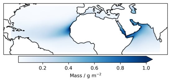
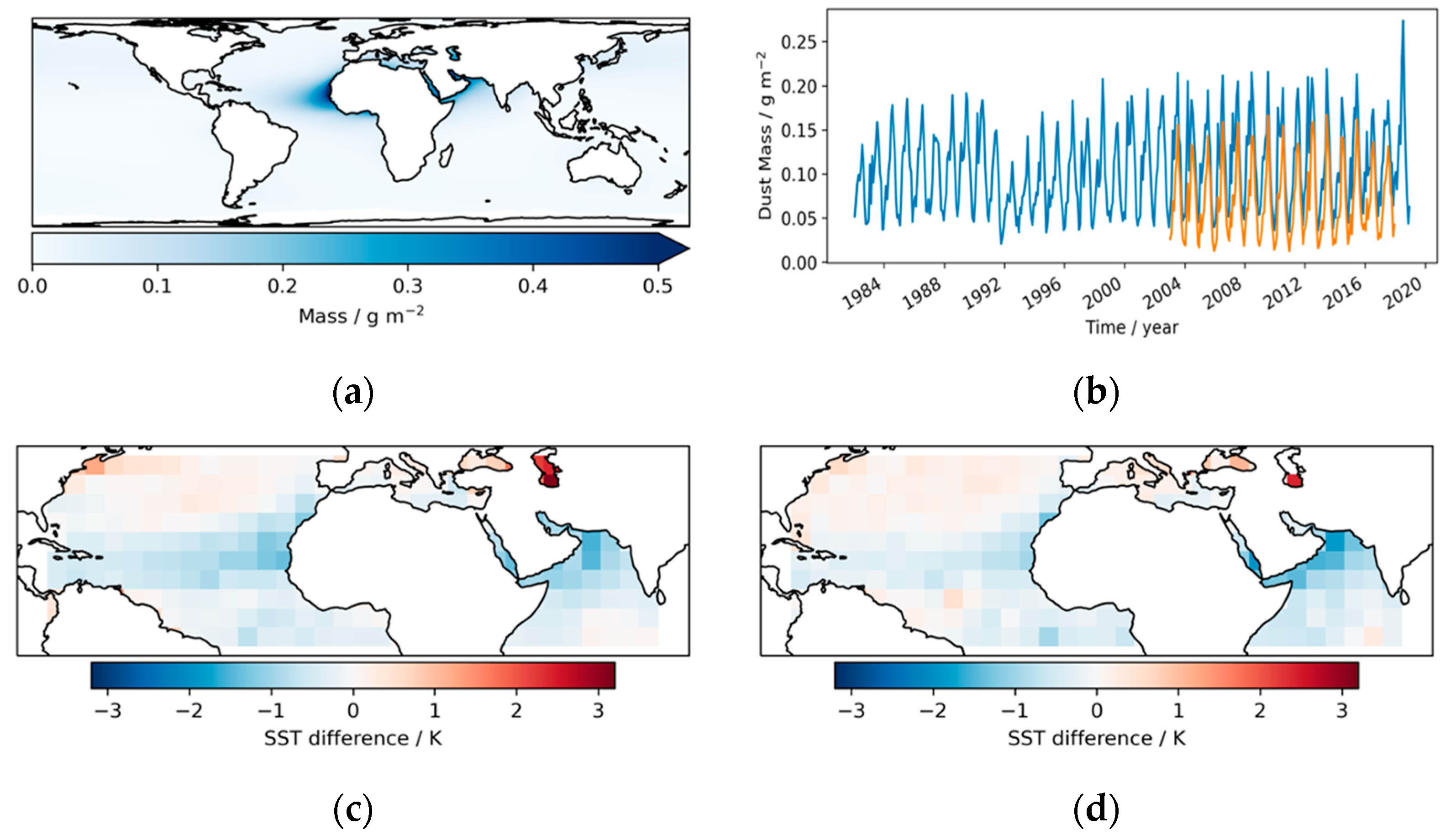
Figure 1 illustrates the context of the paper further, using data whose sources are described in the following section on Data and Methods. Figure 1a shows average column-integrated dust mass over the period 1982 to 2018 inclusive, based on data of the Modern-Era Retrospective analysis for Research and Applications, Version 2 (MERRA-2, Gelaro, et al. [14]). The largest dust loadings over the oceans are associated with transport from the Saharan and Arabian deserts. Significant transport of dust routinely occurs westwards across the Atlantic Ocean at latitudes between 10 and 30°N and reaching the Americas [15,16], and eastwards to the north Arabian Sea. Dust mass is elevated commonly over the Mediterranean Sea, Red Sea, and Persian Gulf, and occasional episodes of dust transport to higher latitudes (e.g., northern Europe) occur. The mass of dust aerosol is highly seasonal, Figure 1b, such that the area-integrated dust mass generally peaks in July. There is also seasonality in dust-plume pathways, however, such that the local seasonal cycle of dust-mass can substantially differ from this integrated picture [17]. In addition to multiannual estimates of dust mass from MERRA-2, the Copernicus Atmospheric Monitoring Service Re-analysis (CAMSRA) [18] dust mass is shown in Figure 1b and presents a consistent picture of the annual cycle and interannual variability, although the mean value is around two-thirds of the MERRA-2 dust loading.

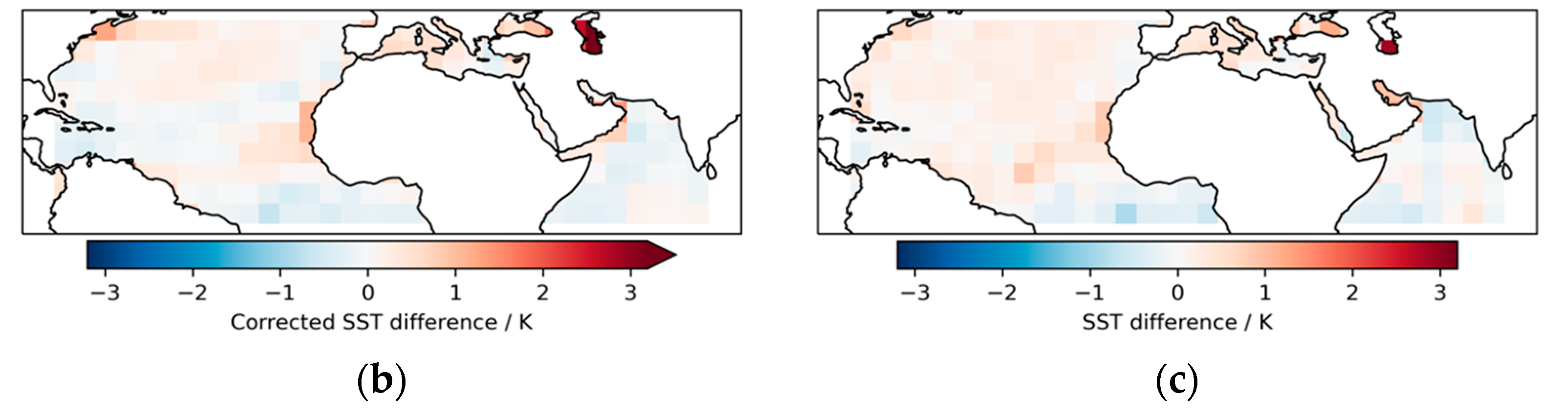
The impact of dust-related errors in infrared SST retrievals on the CCI SST analysis is a cause of significant differences between that analysis and the HadSST4 SST analysis [11,19]. The HadSST4 product, being based purely on in situ observations from instrumented buoys and ships, is not biased by dust aerosol. The largest dust-related differences arise in July and are shown averaged over 8-year periods in the 1980s and 2010s in Figure 1c,d. The in-situ-based analysis is warmer than the satellite-based analysis by up to ~2 K on average in July in areas where dust aerosol is prevalent, with the difference over the Atlantic being more marked in the earlier period than the later period.

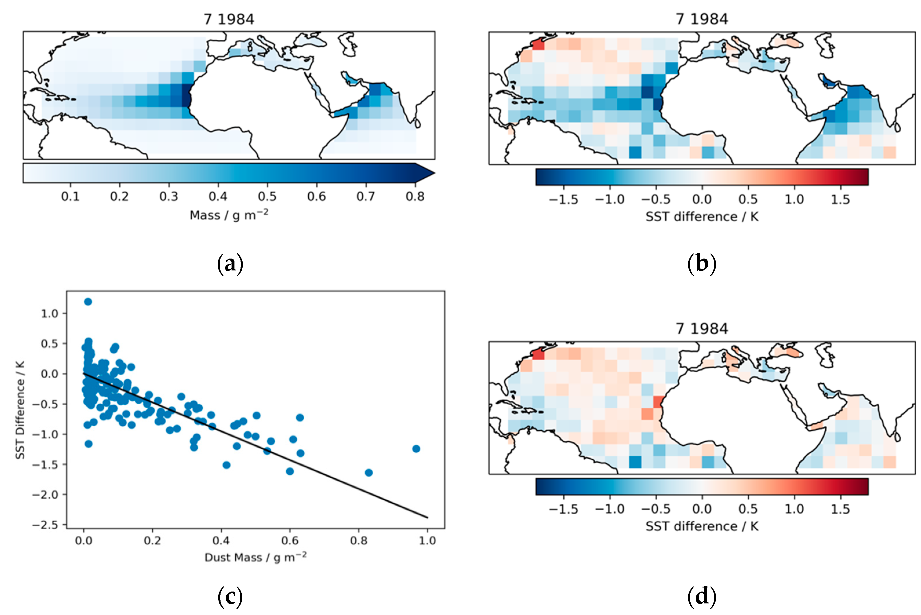
Although the difference is clearly attributable to a dust-related bias in the CCI SST analysis, the true scaling between dust mass and bias is unlikely to be constant, as changes in the vertical distribution of aerosol [20], the aerosol size distribution, and the mix of satellite sensors available to the CCI SST analysis also affect the relationship. However, for the large-scale post-hoc correction derived in this paper, the dust mass in a given month is the key predictor of the required SST adjustment.

This rest of this paper proceeds as follows. The next section describes the datasets used to derive and verify the SST adjustment and the optimization method. Section 3 presents the derivation of the SST adjustment as a function of dust mass. Section 4 addresses a further set of adjustments that become calculable having addressed the dust-related biases. The following section discusses the benefit to applications of the corrected CCI analysis SSTs, the obvious limitations of the approach, and the further work required to remove the need for post-hoc correction for dust biases in a future version of the CCI SST analysis.

2. Data and Methods

The CCI analysis [7] is to be improved with reference to HadSST4 [19], which is a monthly in-situ-based analysis of SST on a 5° latitude-longitude grid, available for download [21]. The CCI analysis is a daily SST product at 0.05° resolution. To re-grid the CCI analysis to the coarser resolution of HadSST4, a re-gridding service has been used that is also available to users of SST CCI products online at http://surftemp.net/regridding/index.html. This service generates netCDF files at spatiotemporal resolutions corresponding to usable multiples of the spatiotemporal resolution of the underlying data.

A variety of effects (sources of error) in both datasets lead to differences between SSTs in CCI analysis and HadSST4. The in situ sources of SST measurements used in HadSST4 are individually biased at some level; bias adjustments are estimated and applied, but residual error will remain. The sampling of SST within a HadSST4 monthly 5° grid cell is not uniform and is of highly variable density between cells. “Ocean” grid cells along coasts may contain a relatively small fraction of sea surface with very few observations. HadSST4 is not interpolated into observation-free cells. While sampling error may be generally expected to be an unbiased effect, in particular cells, this may not be the case: An example could be where many observations come from an intensively used shipping lane whose course does not traverse SSTs representative of the mean SST of the grid cell.

The CCI analysis, in contrast, is interpolated to be gap-free and is obtained from satellite data with a relatively high density of samples. The mean density over the record is 1.1 km⁻² month⁻¹, and therefore, on average, $~3\times {10}^5$ SST retrievals are present per 5° cell per month in the latitudes of interest here. Noise and spatial sampling uncertainty in the SST retrievals are therefore generally negligible, although there will always be exceptions, such as coastal cells with small fractions of sea surface and much lower numbers of observations. Locally systematic errors in the retrieval process (such as the tendency for regional–seasonal components of bias) and large-scale systematic errors (such as overall sensor/retrieval calibration) dominate in the errors in the CCI analysis after re-gridding to the HadSST4 resolution. Away from desert-dust aerosol, these biases are typically ~0.1 K but are greater in some regions that are challenging for retrieval (e.g., persistently cloud areas) and are greater earlier in the record (fewer and more uncertain sensors). Artefacts in the global mean CCI analysis SST in the range of 0.1 to 0.5 K are present during May 1982, during October to December 1982, and during August and September 1983. These “spikes” arise from unstable sensor calibration. Both HadSST4 and the re-gridded CCI analysis come with uncertainty evaluations that account for well-understood error-causing effects, but not covering all artefacts.

Re-analysis fields of desert dust aerosol were obtained from MERRA-2 and CAMSRA, the latter used only as a comparator to the former. MERRA-2 column-integrated dust mass (“DUCMASS”) data [22] were downloaded from https://disc.gsfc.nasa.gov/datasets/M2TMNXAER_5.12.4/summary. These data are monthly averaged on a grid of 0.5° latitude by 0.625° longitude. To use the monthly column integrated dust mass, $M$, as a predictor for HadSST4 versus CCI analysis differences, the MERRA-2 data were resampled to 0.5° by 0.5° using the Python module, xarray (v0.15.1) [23].

The comparison of the regional-mean MERRA-2 and CAMSRA dust mass estimates, Figure 1b, suggests that the uncertainty in the total burden of atmospheric dust mass in the re-analyses is around 30%. Since the SST adjustment developed is a scaling of the dust mass (see next section), a general bias in dust amount is not of concern. The consistency in interannual variability between MERRA2 and CAMS builds confidence in the MERRA-2 dust analysis during the 2000s but begs the question about the realism of interannual variability in the earlier two decades. Interannual variations of dust deposition in the European Alps [24] and Barbados and Miami [15] are not fully consistent with the interannual integrated dust mass, reflecting the fact that both dust mass production and geographical transport of dust are subject to interannual variability. However, the dust deposition records suggest generally elevated dust production during the 1980s compared to the 2000s, reflecting enhanced Sahelian aridity during and prior to the earlier decade. Enhanced dust production during the 1980s is not evident in the analysis dust estimates. In contrast, the dip in dust mass around 1991 to 1993 is also present in the deposition records.

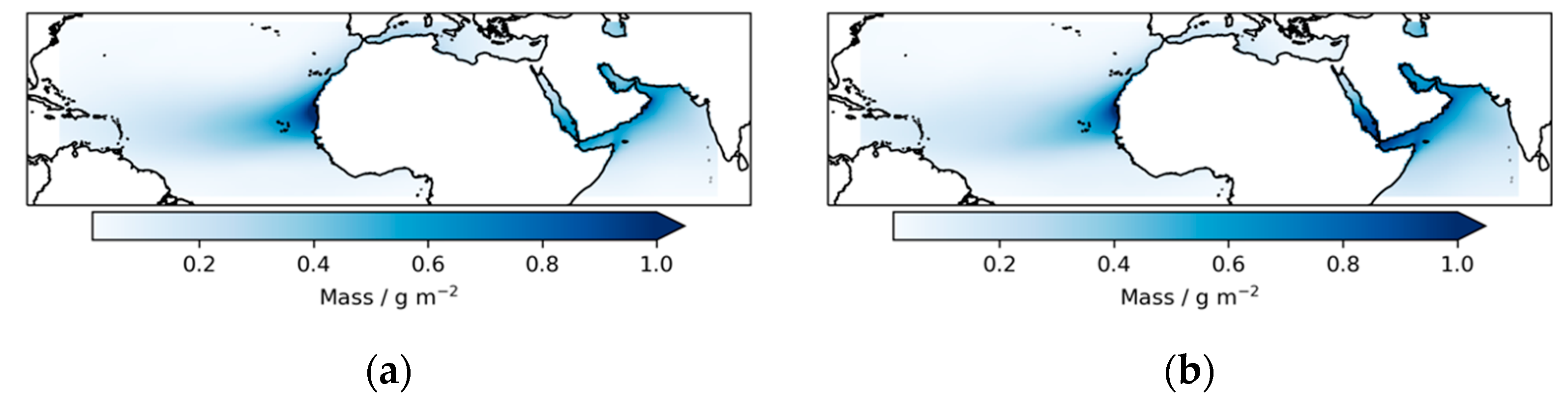
Increased confidence that the interannual spatial patterns of dust mass are usefully (for our purposes) represented in the MERRA-2 analysis is given by Figure 2. Comparison of the dust mass distribution for the 1980s (panel a) to that for the 2010s (panel b) shows greater and farther transport over the Atlantic Ocean in the earlier period, and greater dust loading in the Arabian Sea in the later period. This is consistent with the contrast in the patterns of SST differences evident between Figure 1c,d.

Data analyses were undertaken running Python v3.8.1 in the Scientific Python Development Environment (Spyder 4.1.3). Parameters of the regression model were robustly obtained using Theil-Sen slope fitting [25,26] implemented with the Python package SciPy 1.4.1.

The outline of the methods and results presented in the next two sections is as follows. Since HadSST4 is unbiased with respect to variability in desert dust aerosol or satellite calibration, differences between the CCI analysis and HadSST4 are, at appropriate scales, used to derive empirical adjustments to the CCI SSTs. In Section 3, an adjustment is derived in the form of a time-dependent scaling of dust mass as represented in MERRA-2. This is shown to reduce spatial, seasonal and multiannual signatures of dust-related differences on large scales. Having addressed dust-related errors, Section 4 addresses spurious enhanced variability in the CCI analysis SST that arises from irregular fluctuations in the calibration of the AVHRR sensors, on which we rely during the first decade of the timeseries. The method normalizes the variability of CCI-HadSST4 differences prior to 1993 by global, monthly additive adjustments, such that the statistics of CCI-HadSST4 differences become consistent across the full timeseries.

3. Dust-Mass Adjustment

3.1. Parameterisation

The SST adjustment of the CCI analysis for dust is modeled nonlinearly depending on dust mass, $M\left(x,y,t\right)$, trained on differences between CCI analysis and HadSST4, $\mathsf{\Delta }T\left(x,y,t\right)$. Longitude, latitude, and time are represented respectively by $x$, $y$, and $t$. Deducing an appropriate scaling of $M$ is complicated by the need to avoid confounding by other variable factors. From consideration (not shown) of $\mathsf{\Delta }T$ at tropical longitudes not significantly influenced by desert dust, we know that there may be a seasonal cycle in the difference between the two datasets that varies geographically, arising from a range of effects in both datasets. As noted previously, there are also a few episodes lasting a month or two of large-scale bias in the CCI analysis SST, arising from instrumental instability, and therefore, the global mean bias between the datasets is not constant from month to month. Lastly, the impact of a given amount of dust $M$ varies with a number of geophysical and observing-system factors which change over time, and thus, the scaling cannot be modeled as constant in time.

Given these considerations, the model adopted for SST differences between the datasets is linear:

$$\mathsf{\Delta }\widehat{T}\left(x,y,t\right)=a_0\left(t\right)+a_1\left(t\right)M\left(x,y,t\right)$$

(1)

where $a_0$ is an offset that varies with time, and $a_1$ is the dust scaling factor that varies with time. The dependence of infrared brightness temperature on dust mass for a given atmospheric state is not entirely linear at high dust mass loading [5], but tests in which the dust mass was raised to a power between 0.5 and 1 did not give more convincing results than the linear assumption. We require as many estimates of $a_0$ and $a_1$ as there are months in the timeseries.

3.2. Results

The fitting results are illustrated with regard to July 1984, chosen as a month during the peak-dust season during a notably high-deposition year in both the European Alps and Miami/Barbados records. Figure 3a shows the pattern of dust mass for that month, which is clearly reflected in the pattern of difference between the CCI analysis and the HadSST4 product, Figure 3b. Not all large SST differences are attributable to dust, however, and so, fitting of the relationship (Figure 3c) needs to be tolerant with respect to outliers. The Theil–Sen fitting method estimates the slope of the relationship as the median of the pairwise slopes, giving a regression line that is robust to the high degree of scatter at (in this case) low values of dust mass. Since zero dust loading is assumed to cause zero dust-related bias, the offset is assumed not to be dust-related, and only the slope is relevant to adjusting for dust effects. After correction for dust by addition of $-a_{1}M\left(x,y\right)$, the SST differences show a smaller signature of dust-related biases (Figure 3d). It is possible, given the high deposition in Miami and Barbados that summer, that the MERRA-2 dust plume does not extend far enough to the west, and that this causes the negative differences in SST in the Caribbean partly to remain after adjustment; however, this area of residual bias is no larger in magnitude (being a few tenths of kelvin) than some areas of difference elsewhere. Overall, SST differences are appropriately reduced across the north tropical Atlantic Ocean and across the Arabian, Red, and Mediterranean Seas.

The scale parameter for adjustment, $-a_1$, is shown as a timeseries in Figure 4a. There is an annual cycle in the scaling parameter. Averaged across all years, the scaling is 1.5 around November and 2.0 in June and July. This may reflect annual variations in factors such as size distribution and dust altitude. The estimated scaling of the dust mass was negative for seven individual months, each of them occurring during a low-dust season. This would correspond to a positive SST bias caused by dust. Although a dust plume embedded in a warm air-layer aloft may indeed cause a positive SST bias in infrared retrievals [4], these monthly-scale outcomes seem to be attributable to statistical uncertainty in the regression when the range of dust mass is limited: in six of the seven cases, zero is within the 95% confidence interval for the scale estimate. Therefore, in these cases, the scaling has been constrained to zero, so that adjustments are always zero or positive. The scaling is generally greater during the 1980s than later periods, which may reflect a combination of factors. Possibly, the MERRA-2 dust masses are underestimated during the 1980s. Additionally, the infrared SST retrievals during the 1980s come from single-view sensors only, whereas lower-error dual-view ATSRs and Sea and Land Surface Temperature Radiometers (SLSTRs) contribute data that help to anchor the SST analysis from mid-1991 onwards (except between April 2012 and December 2016, when, again, the scaling is higher). Thus, SSTs before 1991 are on average more sensitive to atmospheric aerosol than during the later years.

Figure 4b,c are post-adjustment equivalents of Figure 1c,d, and illustrate the effective reduction of patterns of difference between the two SST datasets that can be related to desert dust, for Julys during the 1980s and 2010s, respectively. In both cases, there is a tendency to over-adjustment (relative to HadSST4) between the West African coast and Cape Verde islands. This is consistent with plausible expectations such as a proportion of the dust mass in this region being at lower altitudes than further offshore, perhaps reflecting a more local origin for that portion of the total mass.

For climate applications, the long-term stability is important. The stability is the uncertainty in the multidecadal trend arising from error effects in observations. (This is distinct from, but sometimes confused with, the sampling uncertainty in estimation of a trend by regression). The extremely challenging international target for observational SST stability is 3.0 mK year⁻¹ (this being the 2-sigma observational trend uncertainty) [27]. In the absence of any multidecadal traceable reference for SST, comparisons between observational datasets are generally made to assess stability: such comparisons cannot confirm that the stability target is met, but discrepancies larger than the target indicate that the target has not yet been achieved in at least one of the datasets compared and may give an indication of the stability that has been achieved. The mean relative stability between the CCI analysis SST and HadSST4 over the study region is 3.21 mK year⁻¹ before and 3.08 mK year⁻¹ after dust correction, both just outside of the target range at the 2-sigma level. The sign is such that the CCI is warming less than HadSST4. The before-and-after trend values are not statistically different. The dust correction, therefore, does not significantly contribute to reconciling the relative trends of the datasets in the dust region.

4. Calibration-Spike Adjustments

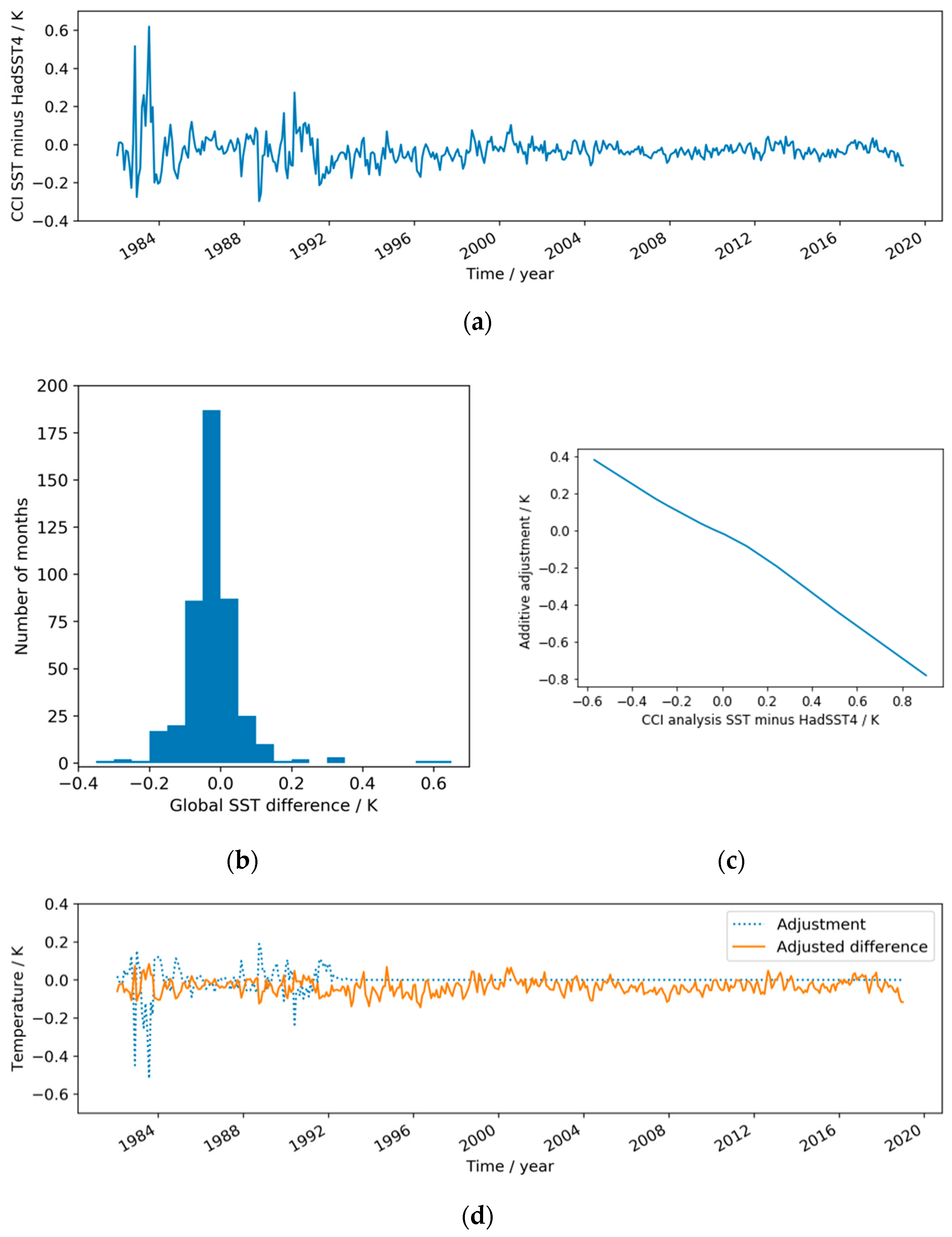
Averaged over the global ocean, dust-bias adjustments are distributed as $0.02\pm 0.01$ K with maximum value 0.08 K. Such adjustments are small but not negligible in the context of monthly global-mean differences between the two SST datasets of $-0.05\pm 0.08$ K prior to dust-bias correction. (Note that the reported “global-mean” values are calculated across the ocean-filled cells north of 50°S where HadSST4 reports an SST, and are area-weighted.) Thus, while not the principle focus of this paper, having a monthly adjustment of the CCI analysis SST for dust mass enables other bias adjustments to be derived with less confounding by dust-related signals. This brief section therefore addresses known global-scale artefacts in SST, mainly identified with excursions in the calibration performance of individual AVHRR sensors in the earliest decade of the record. These “spikes” are evident in Figure 5a and clearly contribute the outliers to the distribution of differences in Figure 5b. Nongeophysical artefacts like this interfere with a range of applications and imply unrealistic fluctuations in global air–sea heat fluxes.

Again, an adjustment for the CCI analysis is derived using HadSST4, using a conservative approach due to the fact that both datasets are subject to uncertainty, particularly in the 1980s, which was a period of rapid evolution of the observing system both in situ and in space. The median and robust standard deviation (scaled median absolute deviation) of the distribution in Figure 5b are $-0.027$ and 0.045 K, respectively. For the period after 1993, the mean and conventional standard deviation match the robust estimates closely, the differences being near-normally distributed as $\mathcal{N}\left(-0.025, 0.046\right)$. A correction is defined to reduce global-mean differences between the datasets. The global adjustment is applied only to the CCI analysis SSTs, since the outliers are attributed to the satellite-based record: We have an identified mechanism (erratic instrumental calibration in individual AVHRR sensors) for such large excursions on the satellite side, but there is no equivalent mechanism for the in situ data record, which averages over the errors of many independent instruments in any given month during the period in question. The adjustment is done by quantile matching. The piecewise linear additive function is found that moves the quantiles of the observed distribution of difference to the corresponding quantiles of a normal distribution $\mathcal{N}\left(-0.035, 0.045\right)$. The adjustment function is shown in Figure 5c. It turns out to be nearly linear. We thereby homogenize the difference distribution of the whole timeseries to that of the more stable period from 1993 onwards.

The adjustment for the CCI analysis needs to be applied at daily resolution. The CCI analysis daily fields are therefore averaged to HadSST4 spatial resolution for each day and differenced from monthly HadSST4 fields interpolated in time to the day (from the central time of each month). The difference is calculated for ocean-filled cells north of 50°S where the time-interpolated HadSST4 dataset has an SST, on an area-weighted basis. The global offset adjustment is applied to all SSTs in the CCI analysis, except: (i) areas where the adjusted analysis SST registers less than 271.35 K (the typical freezing temperature of seawater) which are reset to 271.35 K to avoid unphysical subfreezing values; (ii) there is a linear tapering of the adjustment during 1992 with zero adjustment made from 1993 onwards. The adjustment timeseries and post-adjustment SST difference are shown in Figure 5d.

5. Comparison of Analysis and Drifting Buoy Data

To investigate the impact of the combined dust and spike adjustments on the CCI analysis SSTs, comparison is made to drifting buoy measurements of SST from the Met Office Hadley Centre Integrated Ocean Dataset (HadIOD) v1.2.0.0 [28]. This is not a fully independent comparison, since HadSST4 uses drifting buoy data, as well as other sources of data such as ship engine intakes, each source having different strengths and weaknesses [29]. The comparison here is performed as follows. Quality controlled drifting buoy SSTs are averaged by platform identifier and UTC day, to create “daily” buoy SSTs are their daily-mean location. In recent decades, most platforms have been reporting at least hourly data, whereas in the early part of the record, a daily value will typically be based on 1 to 4 buoy measurements. The daily buoy value is matched to the day and latitude–longitude cell of the CCI analysis and the SST difference found. For interpretation, averages across these differences are then calculated for subsets in time, space and (not shown here) geophysical factors such as wind speed or atmospheric water vapor.

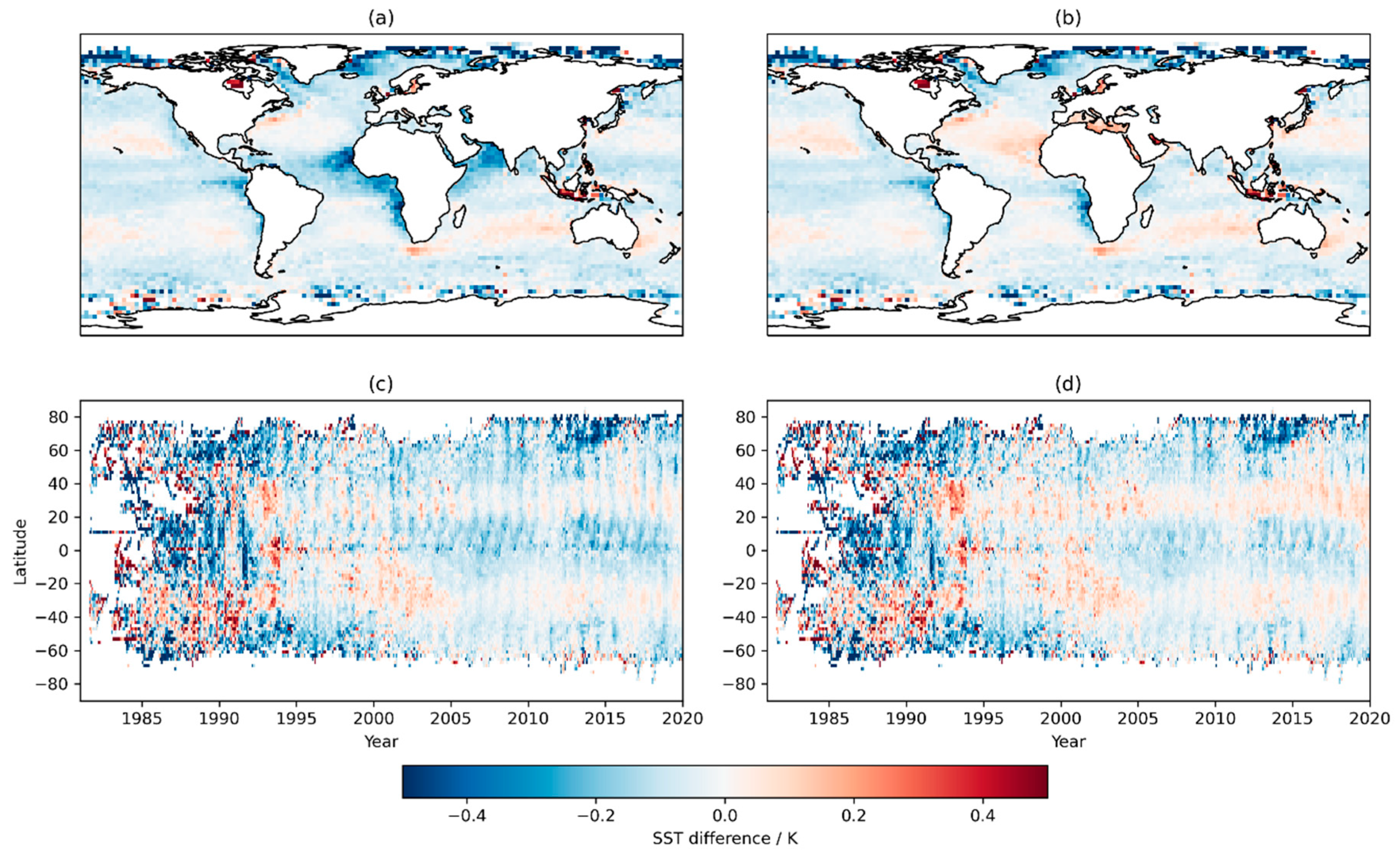
The results of the comparison are shown in Figure 6. Note the stretched scale on which the differences are plotted, to enable distinction of mean differences of 0.1 K or less. Comparison of panels (a) and (b) shows that a dust-related pattern of cool analysis SSTs clearly corresponds geographically to the main dust-mass areas in Figure 1a and is greatly reduced by the dust-mass adjustment. The latitudinal–seasonal distribution of this improvement can be seen from panels (c) and (d), with a reduction in the negative zonal-mean differences and their amplitude of seasonal variation in the latitudes between the equator and 20°N. There is also a reduction in the negative zonal-mean differences during summer in latitudes from 20 to 50°N. This arises because of summer-season elevation of dust transport from Asia across the north Pacific: although not tuned to this area, the dust adjustment is applied globally and has a small beneficial impact to reduce negative SST biases across the North Pacific in summer.

These points are most readily seen in the data from around 2000 onwards, by which time the number of buoys reporting had increased to higher levels that have since been broadly maintained. The results are noisier prior to 2000 and become much sparser in the 1980s. The first standardized design of drifting buoys measuring SST was introduced with the Surface Velocity Program, deployed from 1993 onwards and reaching target levels of completeness by September 2005 [30], meaning that sparsity and possibly uncertainty of the in situ SSTs increase when considering earlier times within the record. For this reason, the benefits of the spike adjustments are more difficult to discern, the most clear being the effect of positive adjustments applied during 1988, which mean a vertical strip of negative SST difference evident in panel (c) during that year is not visible in panel (d).

Overall, the comparison supports there being a positive impact of the adjustments for the CCI analysis.

6. Discussion

Two empirical adjustments to the CCI analysis SST v2 have been defined in this paper. These adjustments address biases from specific error effects in the SST retrieval algorithms used for the v2 climate data record: cold biases due to the unaccounted-for absorption of IR radiance from the sea surface by desert-dust aerosols; and temporary large-scale fluctuations in the calibration of specific AVHRR instruments, to which the SST record is particularly susceptible in the 1980s, prior to the availability of more robust dual-view sensors and when in v2 we are mostly reliant on a single AVHRR instrument at a given time [7].

The empirical adjustments apply to large and global scales and have been quantified with reference to a monthly in situ SST product, HadSST4. It is not ideal to reduce the degree of independence between these two representations of global SST in this way. A high level of consistency between timeseries that have a high degree of independence gives confidence in our quantification of the climate over recent decades. It would be far more satisfactory to improve the robustness of the CCI analysis SST to desert dust at the point of retrieval and to make the data less prone to the fluctuations of calibration in individual satellite sensors. Work in these directions is ongoing in preparation for the v3 climate data record from SST CCI.

The empirical approach to adjustment has the advantage of bypassing complicating factors such as ensuring adequate representation in radiative transfer of the effects of irregular dust particle shape [31] and extremes of the size distribution of particles [32]. However, a limitation of our approach is that these empirical adjustments are derived using only the Saharan-dust region where the “signal-to-noise” is clearest. The adjustment is applied globally, including across the north Pacific Ocean and around Australia, where dust properties and profiles may differ. Although, in MERRA-2, the dust loadings in these areas are less than over the north Atlantic (which, if correct, makes any error in the adjustment less critical), some studies have reported relatively higher estimates of dust deposition elsewhere [33].

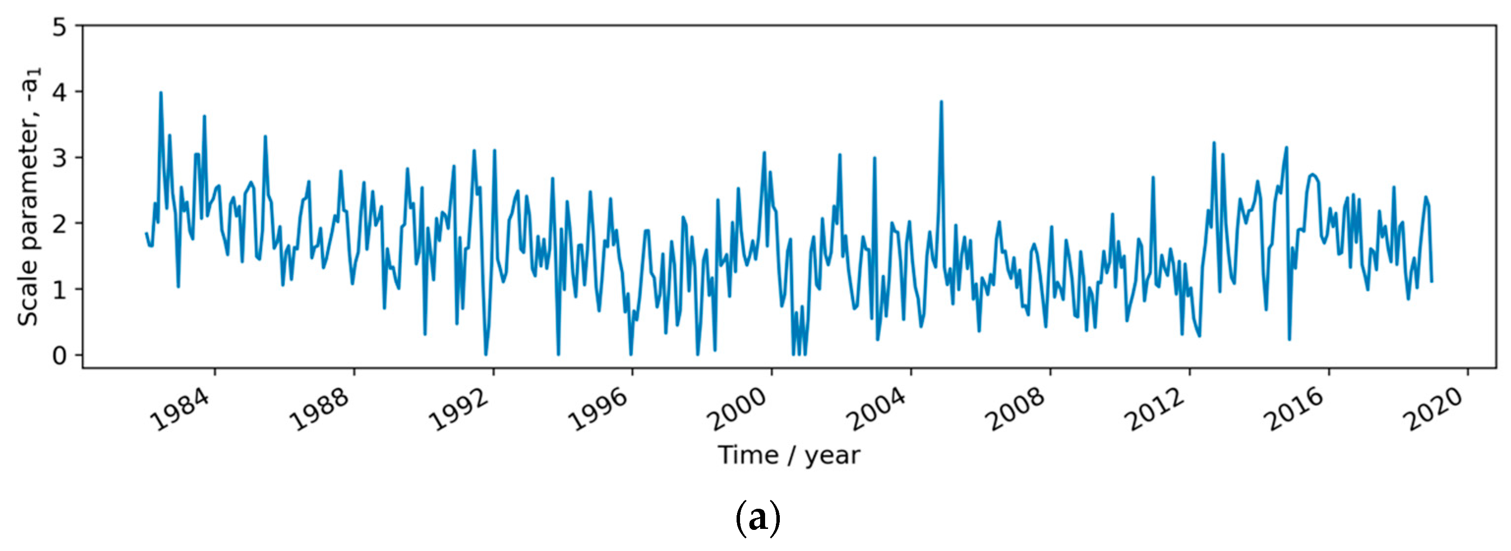
What are the uncertainties of the CCI analysis SSTs after adjustment? The adjustments for dust are made on a monthly 5° scale, while dust amounts in the atmosphere vary daily on scales of 1 to 100 km. The shorter-scale dust variability causes fluctuations in retrieved SST on the same scales. As with all SST CCI products, the analysis SSTs are provided with per datum evaluations of uncertainty [34]. The CCI analysis system generates the uncertainty estimate given the number of SST observations available and their variances, considering scales up to ~100 km and 3 days. The uncertainty from shorter-scale dust-related variability is therefore represented in the products by increased values of the estimated SST uncertainty in dust-affected regions. The uncertainty estimates provided in the CCI analysis dataset do not account for monthly 5°-scale biases from dust, either before or after dust-bias adjustment. To form an estimate of the additional uncertainty from the residual large-scale biases from dust that remain after dust-bias adjustment, a confidence interval on the Theil–Sen estimate of the monthly scaling is available. Expressing the confidence interval as a fractional uncertainty, $f_1$, in the scale parameter, enables spatiotemporally resolved estimation of uncertainty in the dust-bias correction as $\left|f_1{a}_1\left(t\right)M\left(x,y,t\right)\right|$. The mean value of the fractional uncertainty is $f_1=$26%. The global-scale uncertainty after adjustment for the spikes in AVHRR calibration is difficult to quantify. While we do account for normal levels of satellite calibration uncertainty in the SST products used in the analysis, the uncertainty model does not account for periods of anomalous calibration such as those associated with the spikes, although some progress toward doing so has been reported [35]. What can be said is that the uncertainty evaluations provided in the CCI products are likely to be more representative after the spike adjustments than before, since the adjusted-for spikes were not accounted for in the uncertainty model.

In this paper, HadSST4 is used to improve the CCI analysis. It is worth noting, however, that the two datasets are mutually informative. At 5° monthly resolution in ocean regions where sampling density is low, the HadSST4 uncertainty can be large compared to the magnitudes of large-scale temperature adjustment discussed here. In these circumstances, the much smaller sampling uncertainty on a monthly-5° scale from the CCI analysis SST means the satellite product is informative about the errors in the in situ product. Having alternative realizations of the history of global SST based on very different methodologies is beneficial for mutual improvement, through comparison based on understanding of their strengths and weaknesses.

Although it would be more satisfactory if they were not required, the empirical adjustments reported here are useful as discussed below, firstly, for users of the CCI analysis, and secondly, as a contribution to preparation for the v3 products from SST CCI.

There are many uses of multidecadal daily SST products at spatial resolution of <1° latitude–longitude—finer resolution than can be generated globally from in situ sources of data alone. Moreover, some of these applications also demand high observational stability over several decades, because both the daily <1° evolution and the long-term climatological variability at that scale are important. An example is the characterization of the degree of extremity of SST variability—i.e., identifying and quantifying marine heatwaves (MHWs) [36,37,38]. The importance of MHWs is often ecological: coastal and near-surface ecosystems are adapted to the SST climatology of the past, and increasing exposure to MHWs [39] under climate change is already driving ecological changes that are sometimes sudden and dramatic [36,40,41,42,43]. Duration and intensity are both important for characterizing the stress which a MHW places on an ecosystem. Duration needs to be resolvable at the daily level [37]. For long-lived, static biota—particularly corals—adaptation by migration is not possible when SST change is significant within decades [44], and quantifying the SST climatology to which coral reefs are adapted requires stability and fine (<0.25°) spatial resolution [45]. For such purposes, the adjustments to the CCI analysis described here should be advantageous, through reduction of spurious dust variability (e.g., in the Red Sea) and improved observational stability during the 1980s.

The adjusted version of the CCI analysis SST will also provide a platform for an improved v3 climate data record, which is on schedule for production during 2021. The AVHRR SSTs are obtained using optimal estimation [46]. The retrievals benefit from having a low-bias prior SST in two regards: this supports effective cloud detection [47] and supplies a good point around which to linearize the optimal estimate. The degree to which the retrieved SST is directly sensitive to the prior is generally <5% for the highest quality of data in the CCI system [7]. This means that typically up to $\frac{1}{20}$th of any error in the prior SST is propagated to the retrieved SST. The adjusted CCI analysis v2 will be used as prior for v3, and therefore, the reduction in large-scale SST errors from the dust and spike issues will contribute to minimizing prior error propagation to the v3 results. Other improvements to the SST retrieval methodology will be incorporated, including better estimation of satellite bias and error covariance characteristics [48], as well as increasing the number of sensors used for SSTs through the 1980s, to reduce the impact of calibration bias problems that arise in individual sensors.

To make the SST CCI analysis more readily accessible to some users who do not require the full daily 0.05° resolution of the timeseries, a service to obtain the data re-gridded to coarser resolution is available at http://surftemp.net/regridding/index.html. At the time of writing, work is ongoing to make the adjustments (including associated additional uncertainty) described in this paper selectable as options for users of that service.

7. Conclusions

The presence of desert-dust aerosol is a cause of bias in satellite infrared retrievals of sea surface temperature used in a multidecadal analysis, namely, the SST CCI analysis. The main areas affected are the tropical north Atlantic Ocean and the Mediterranean, Red, and Arabian Seas, where on a monthly average scale, the temperature analysis was biased cold by amounts typically in the range 0.1 to 2 K. The multiannual dust mass patterns obtained in a global reanalysis (MERRA-2) correlate with dust-related differences between the CCI analysis and a coarse scale in-situ-based product, HadSST4, meaning that a scaling of the dust patterns to give a temperature correction for the CCI analysis improves their agreement. Other global-scale biases are also evident in the difference of the dataset, and these are interpreted as intermittent deviations of satellite calibration, particularly for the 1980s when the CCI analysis v2 is often reliant on a single satellite mission at a given time. A global adjustment as a function of CCI minus HadSST4 difference is derived to reduce the spurious variability associated with these “spikes” in calibration.

The corrections described are beneficial to applications of global SST timeseries that require daily, relatively high spatial resolution combined with long-term data of good observational stability, such as assessing ecological responses to marine heatwaves.