The Design a TDCP-Smoothed GNSS/Odometer Integration Scheme with Vehicular-Motion Constraint and Robust Regression


Abstract
1. Introduction
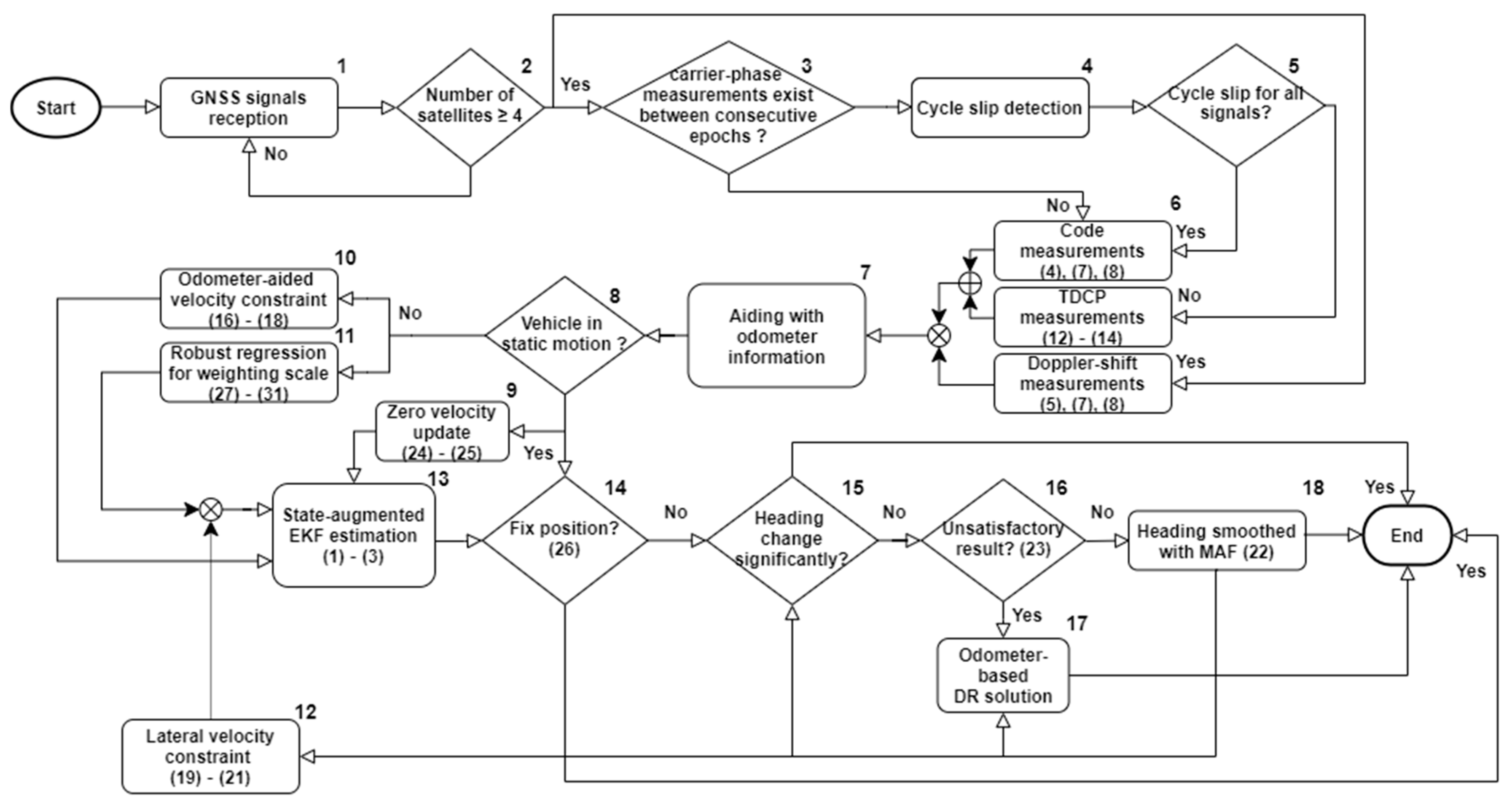
2. Methods
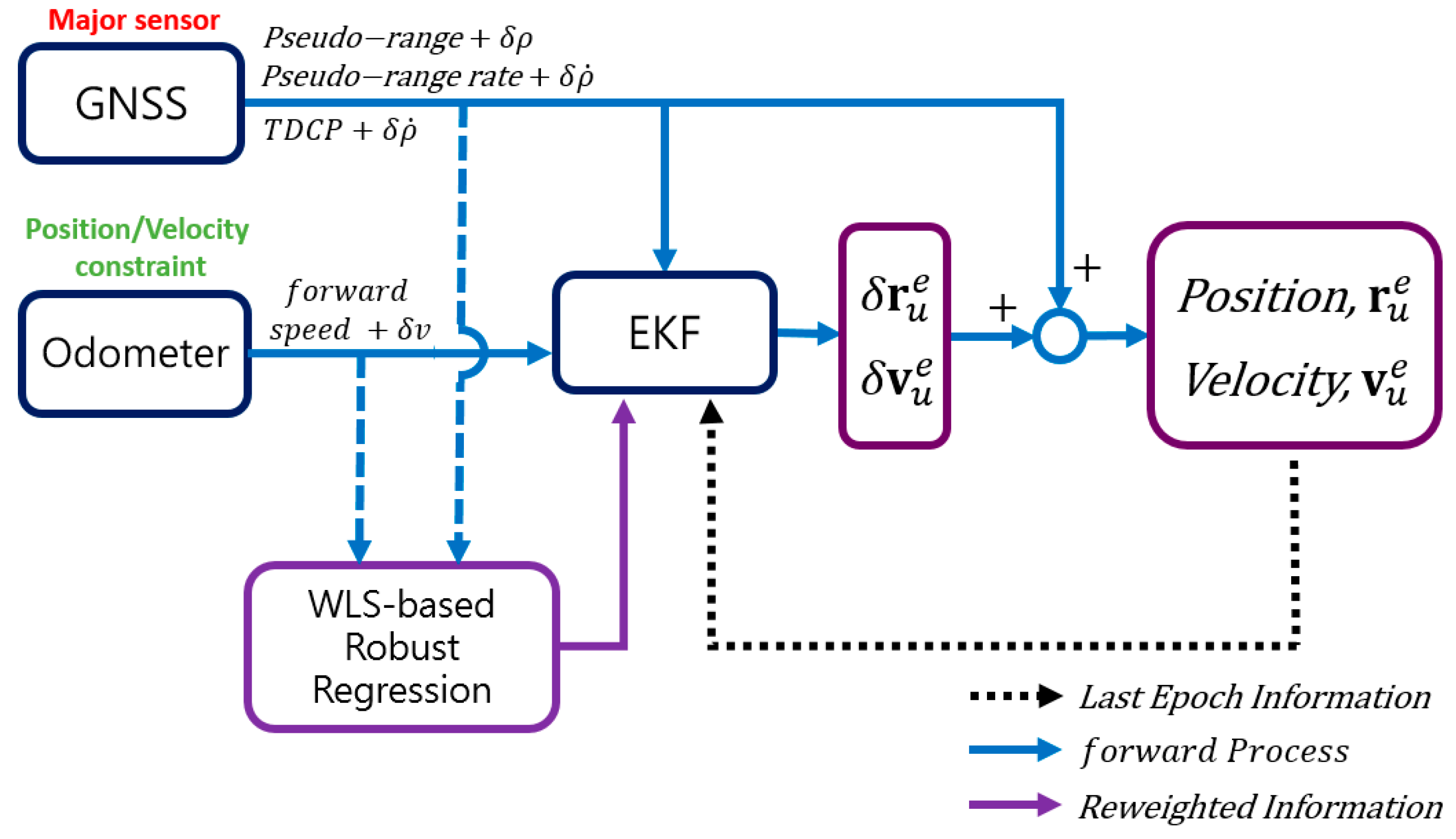
2.1. State-Augmented EKF Design
2.2. Measurement Model for Pseudorange, Doppler Shift, and TDCP
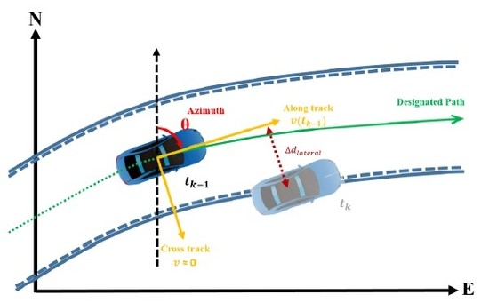
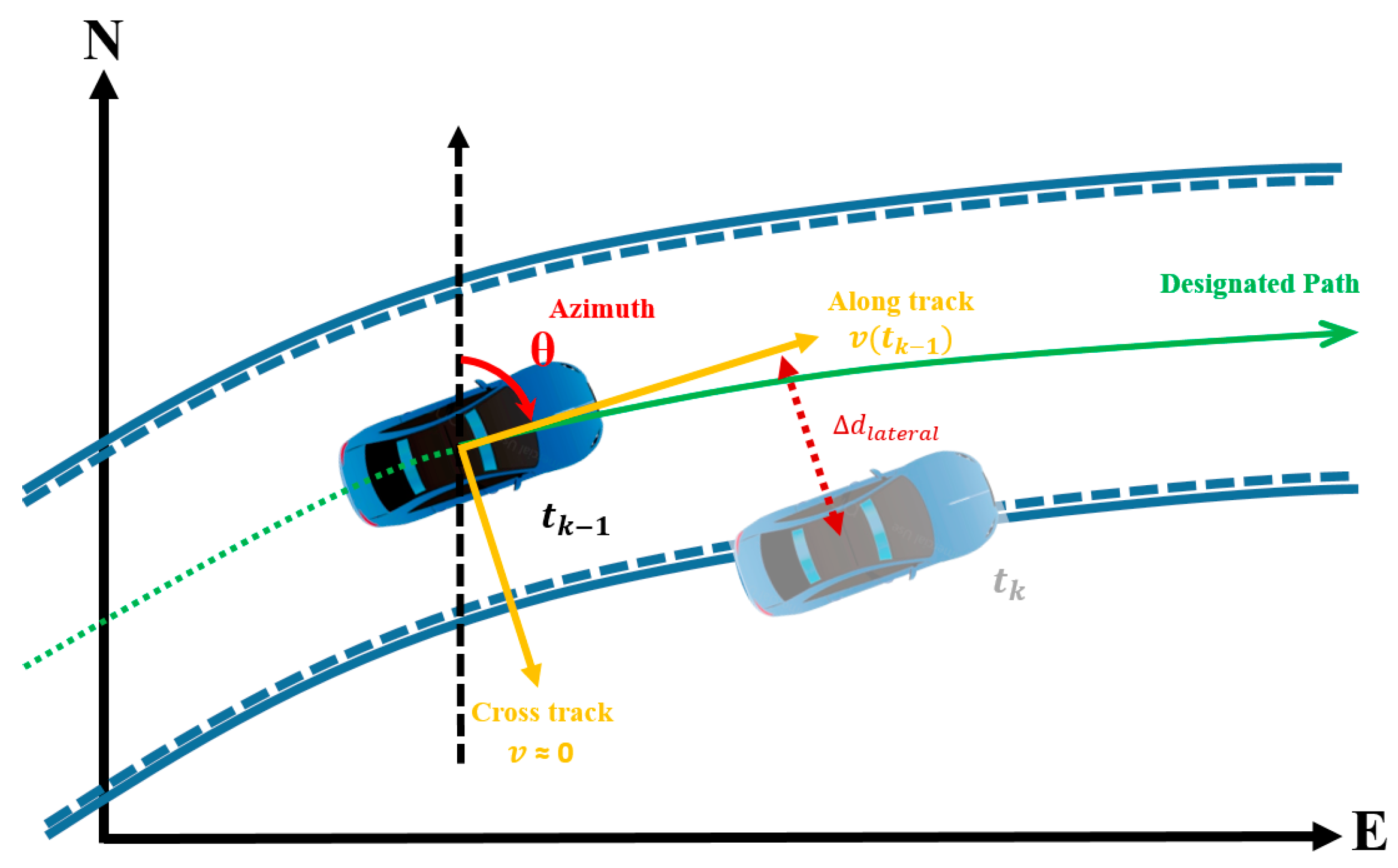
2.3. Measurement Model for Odometer Observation with Vehicular-Motion Constraint
2.4. Robust Regression with Odometer Aiding
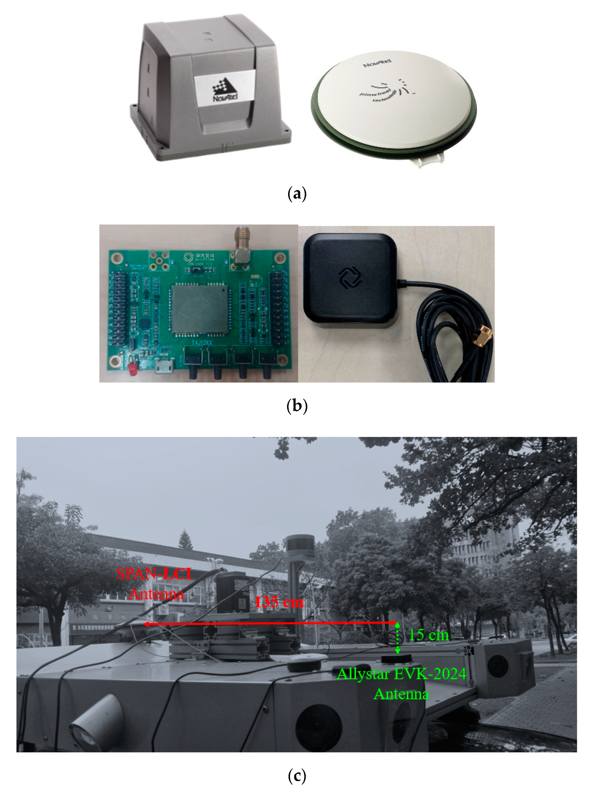
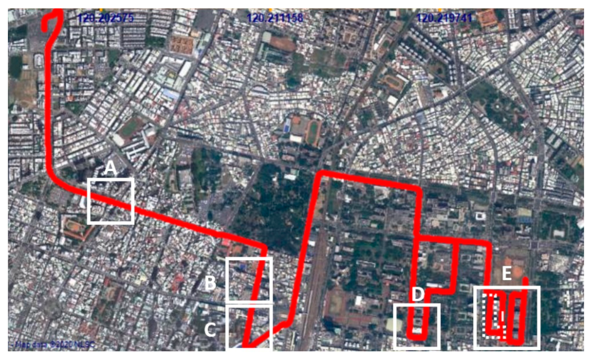
3. Experiment
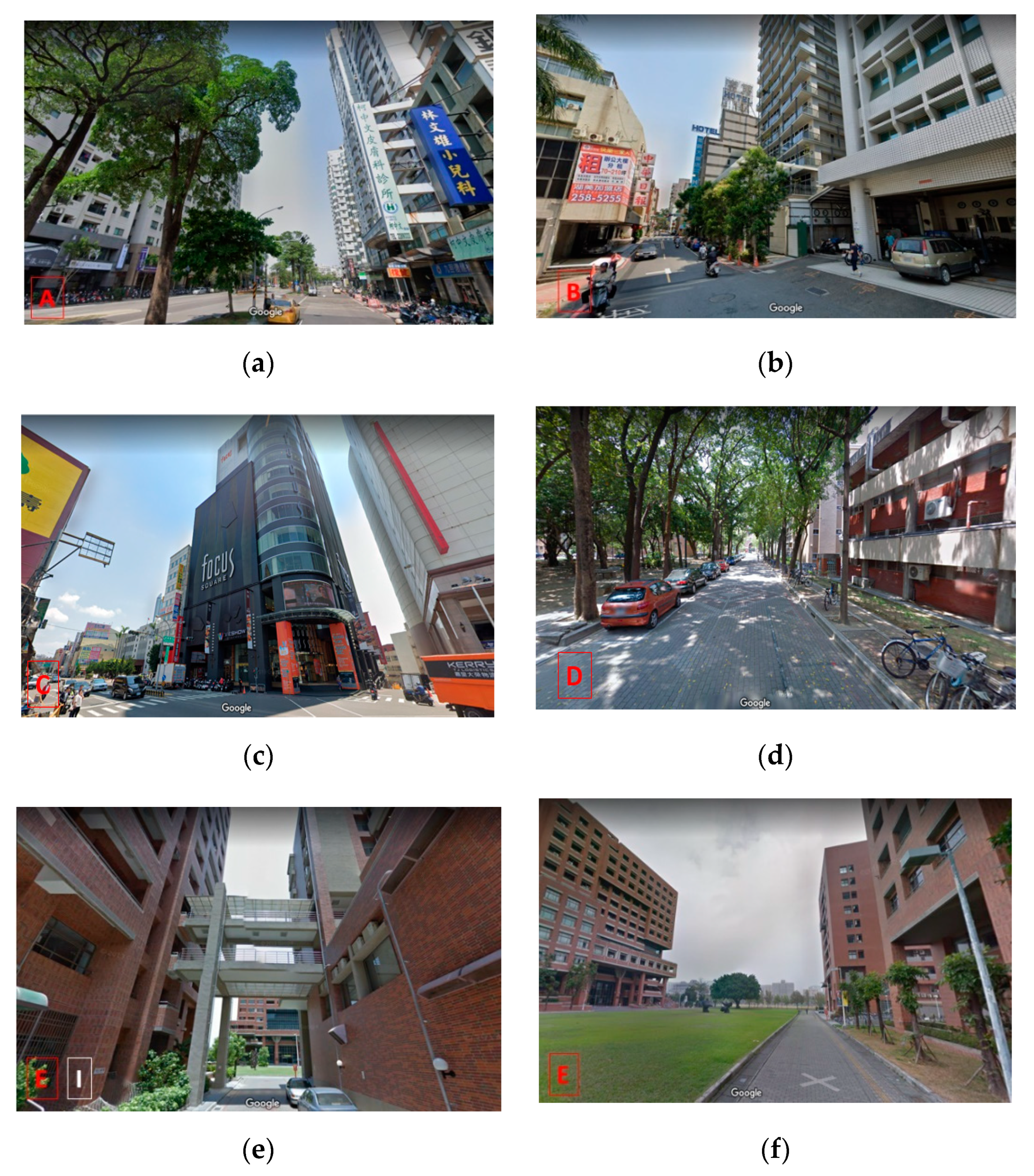
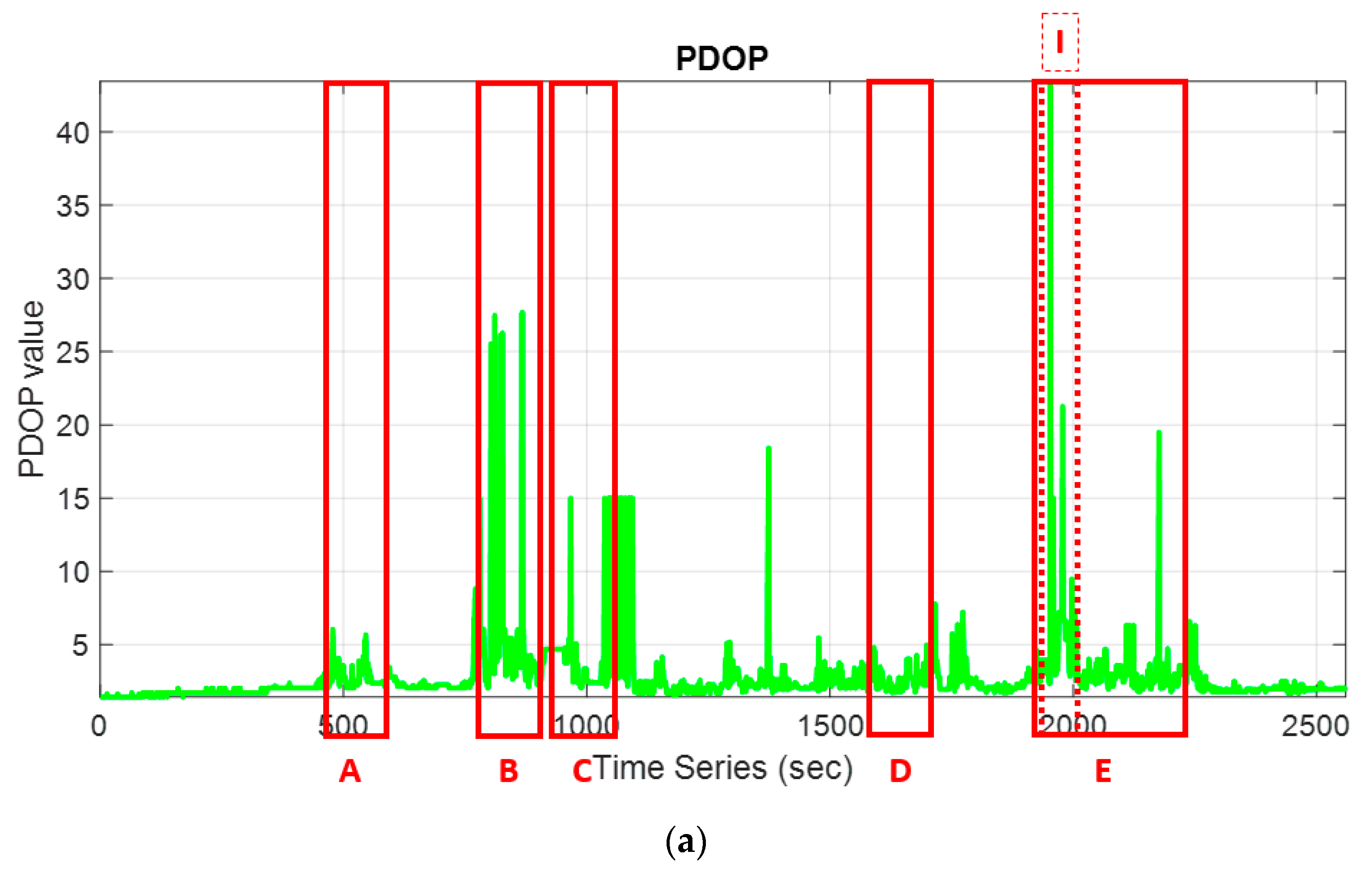
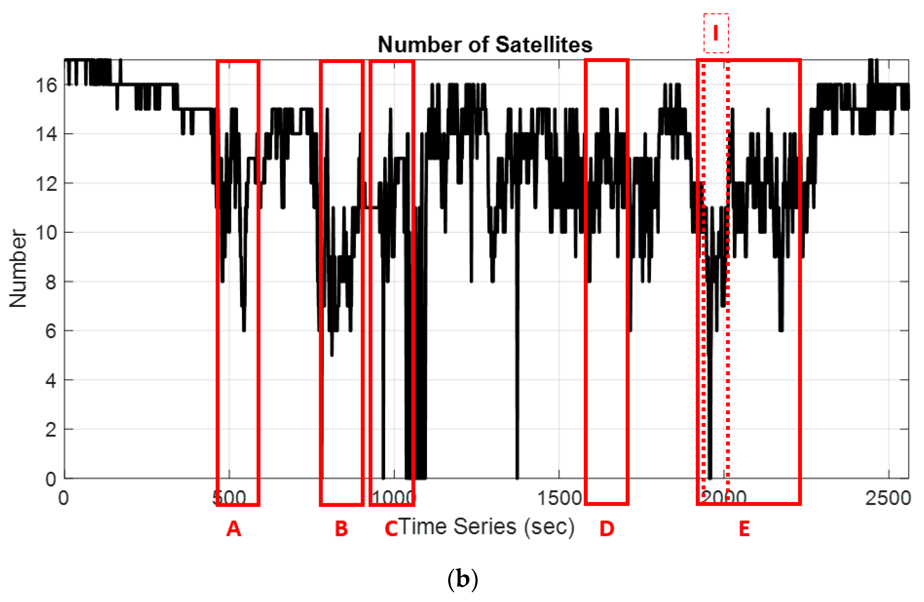
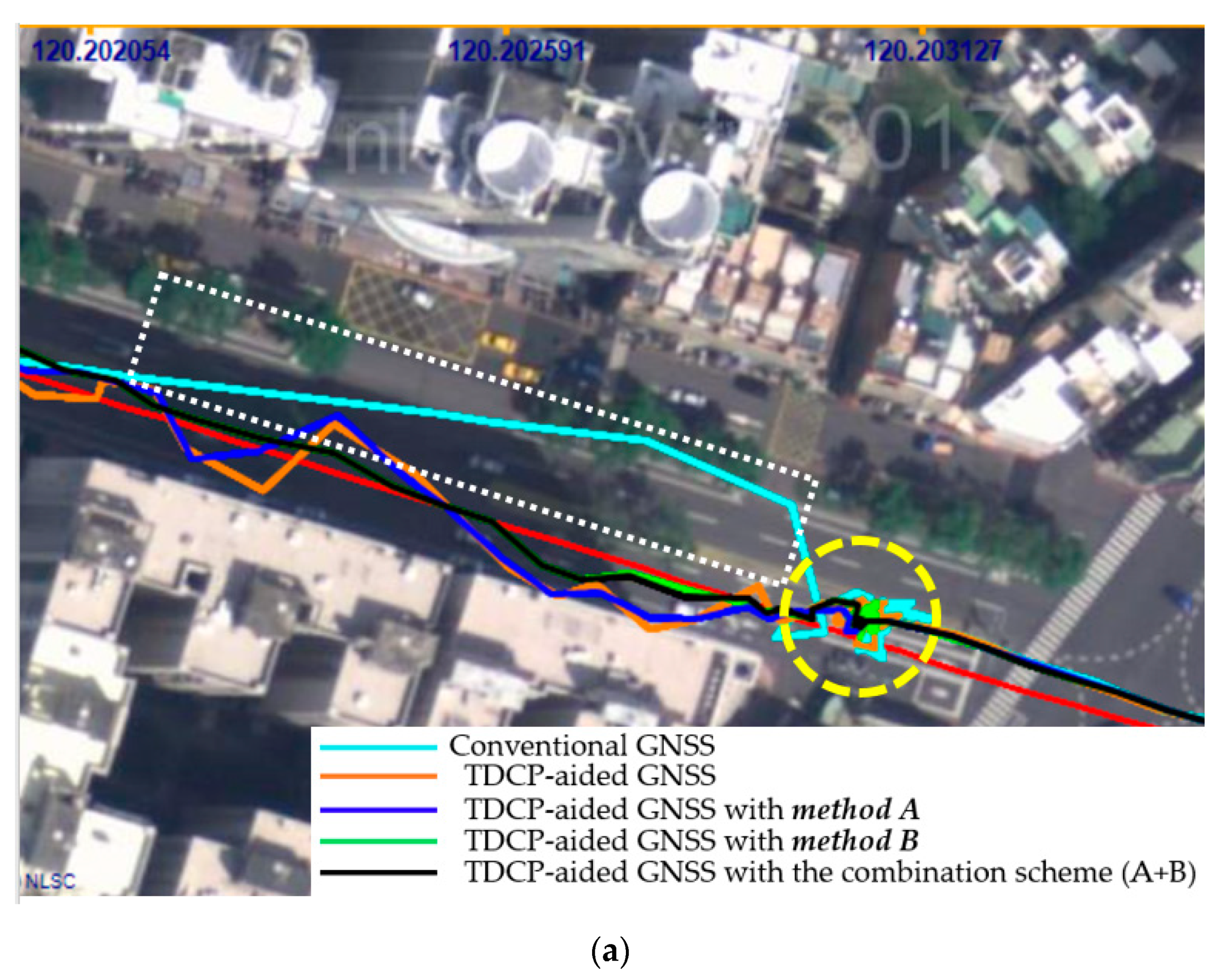
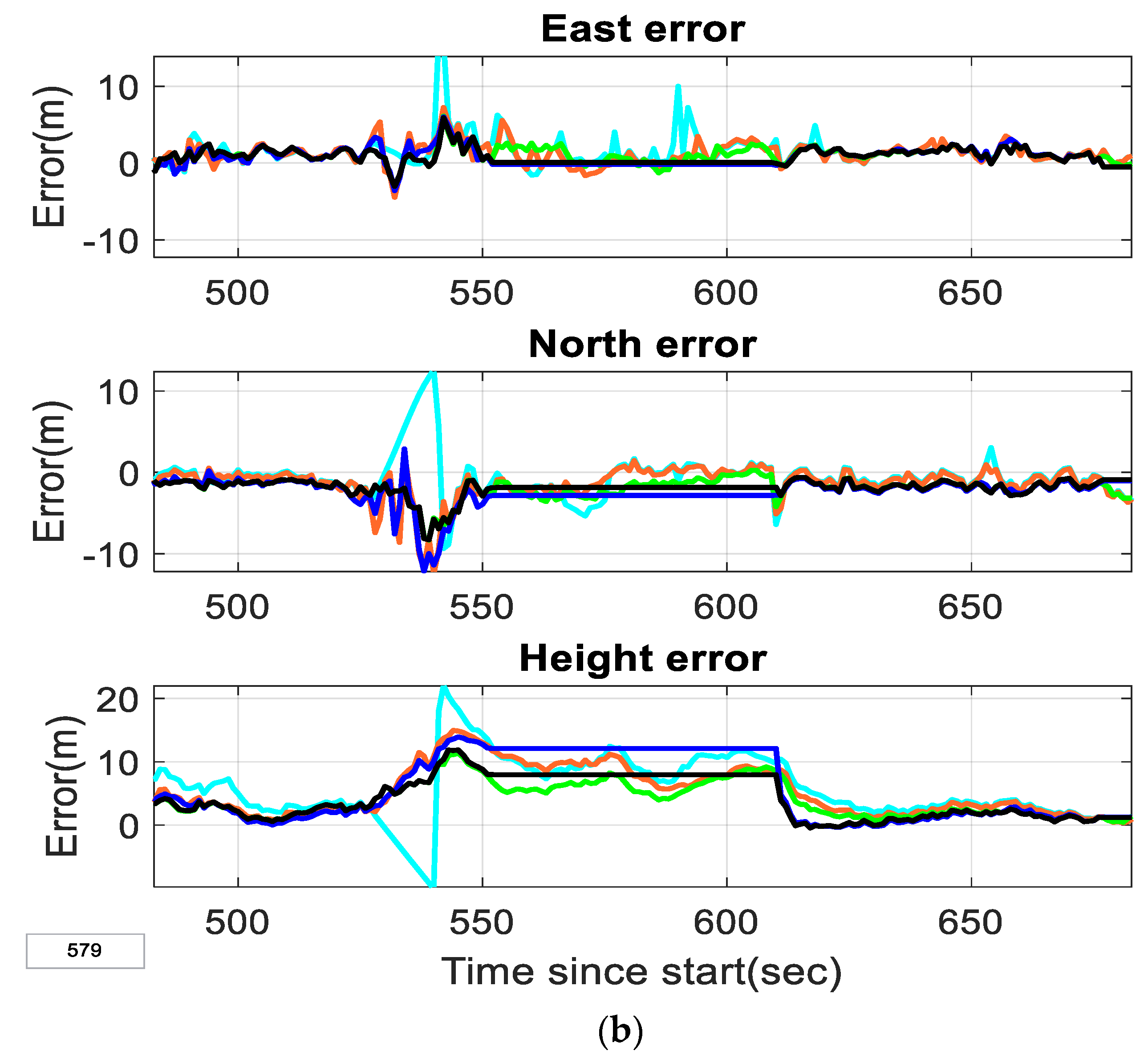
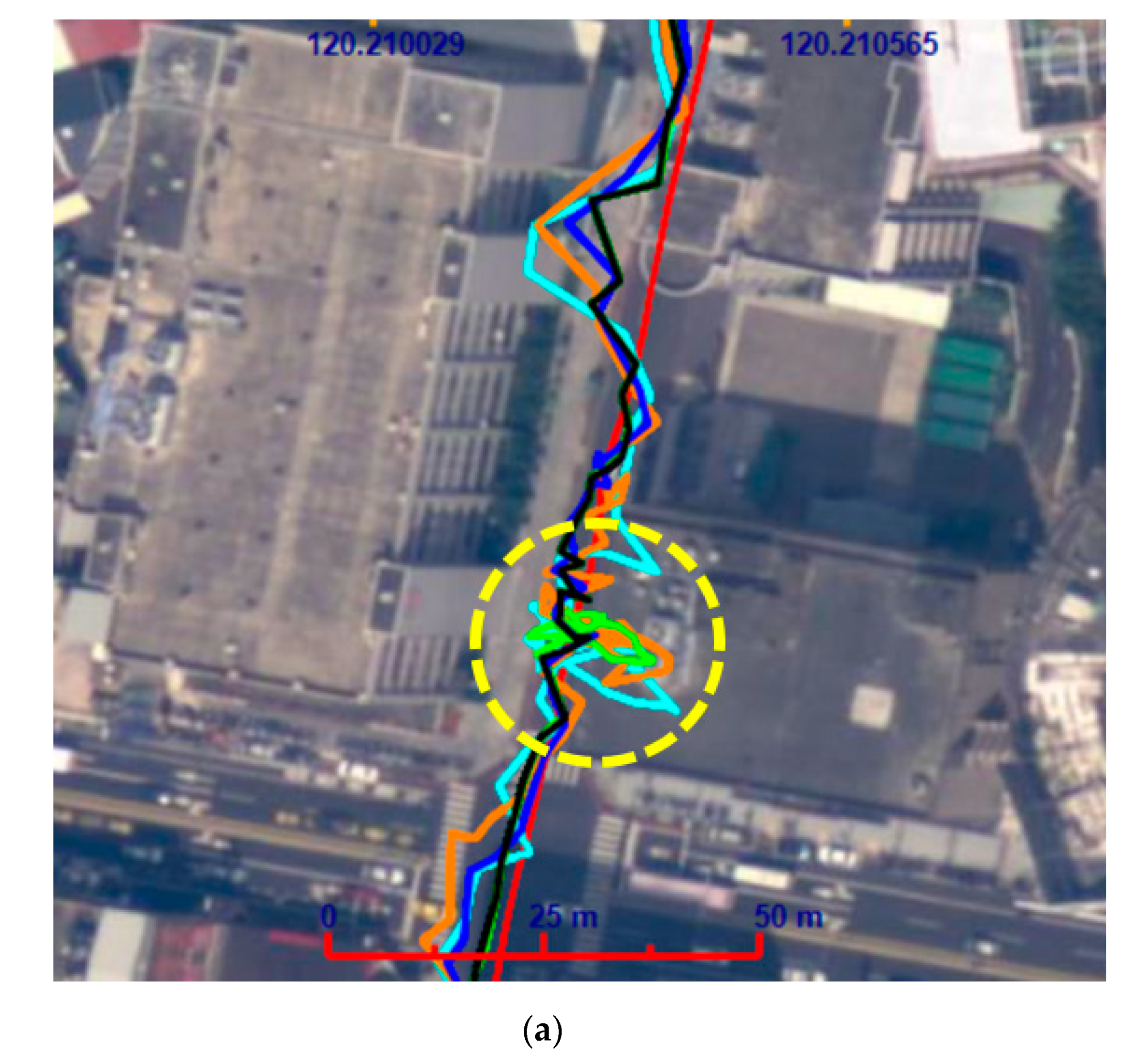
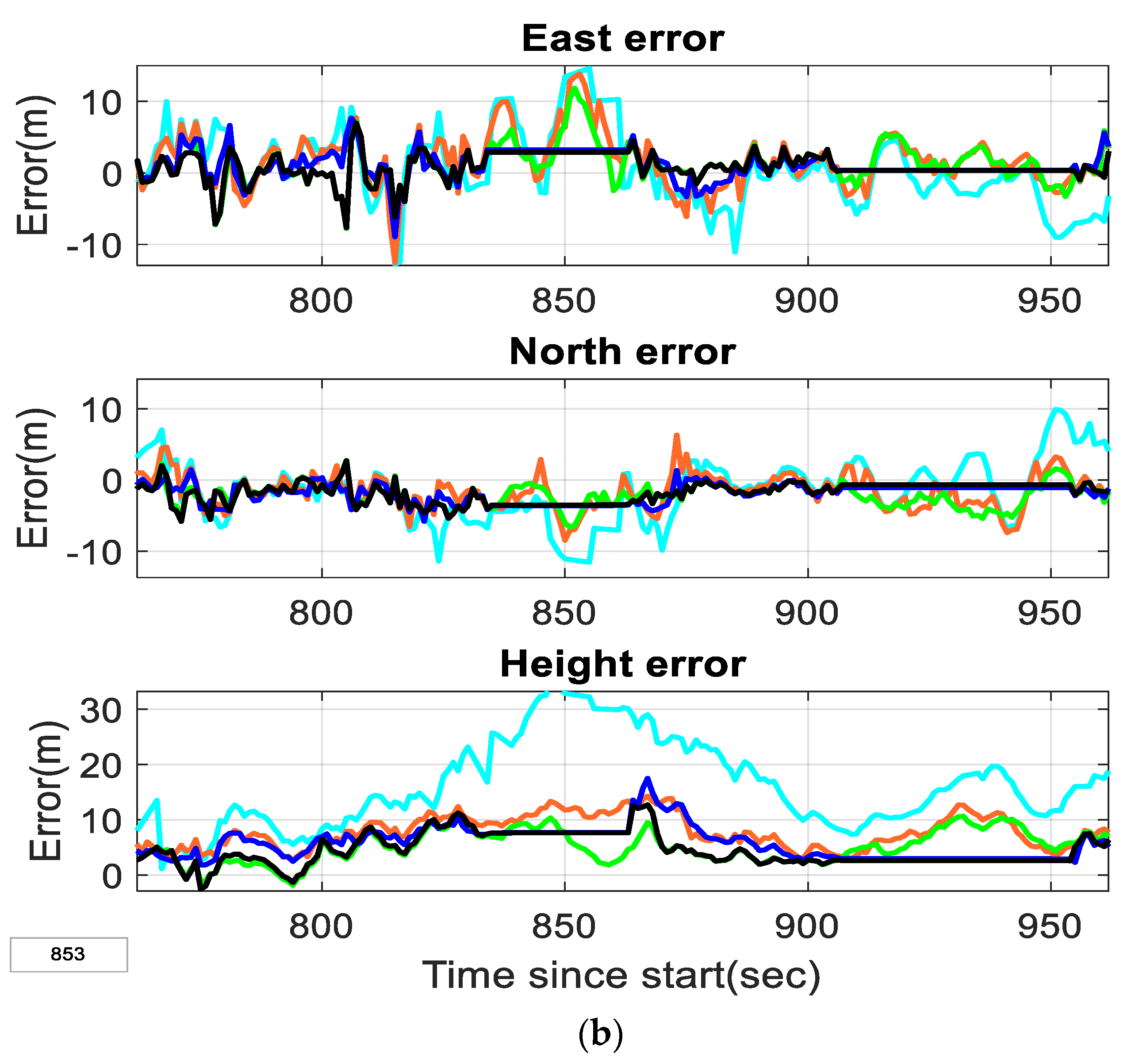
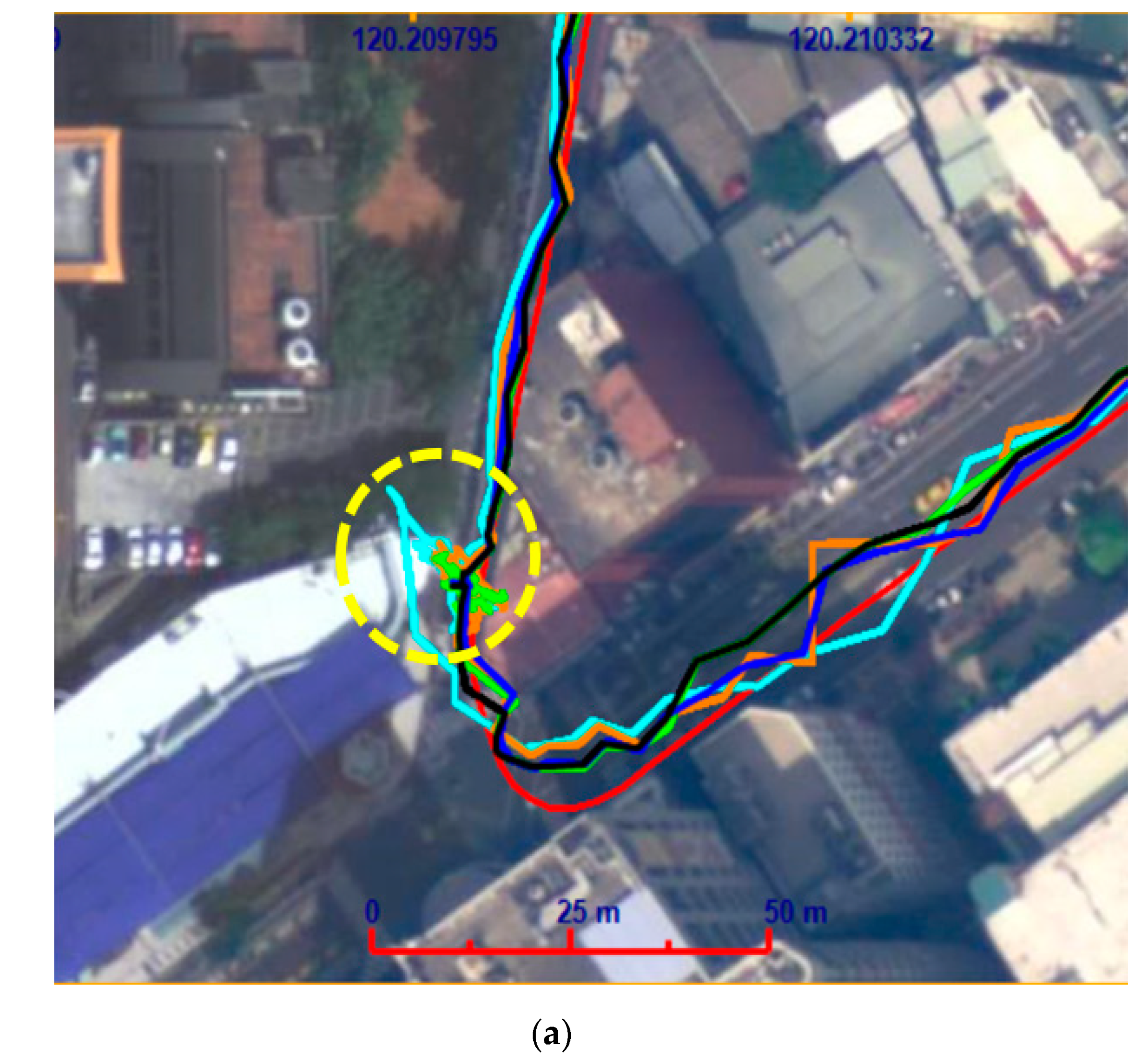
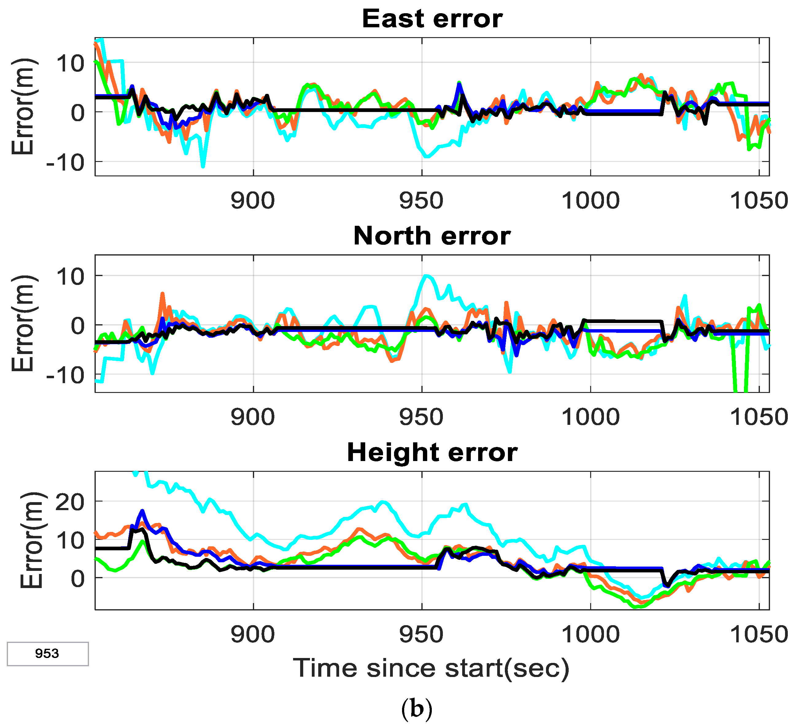
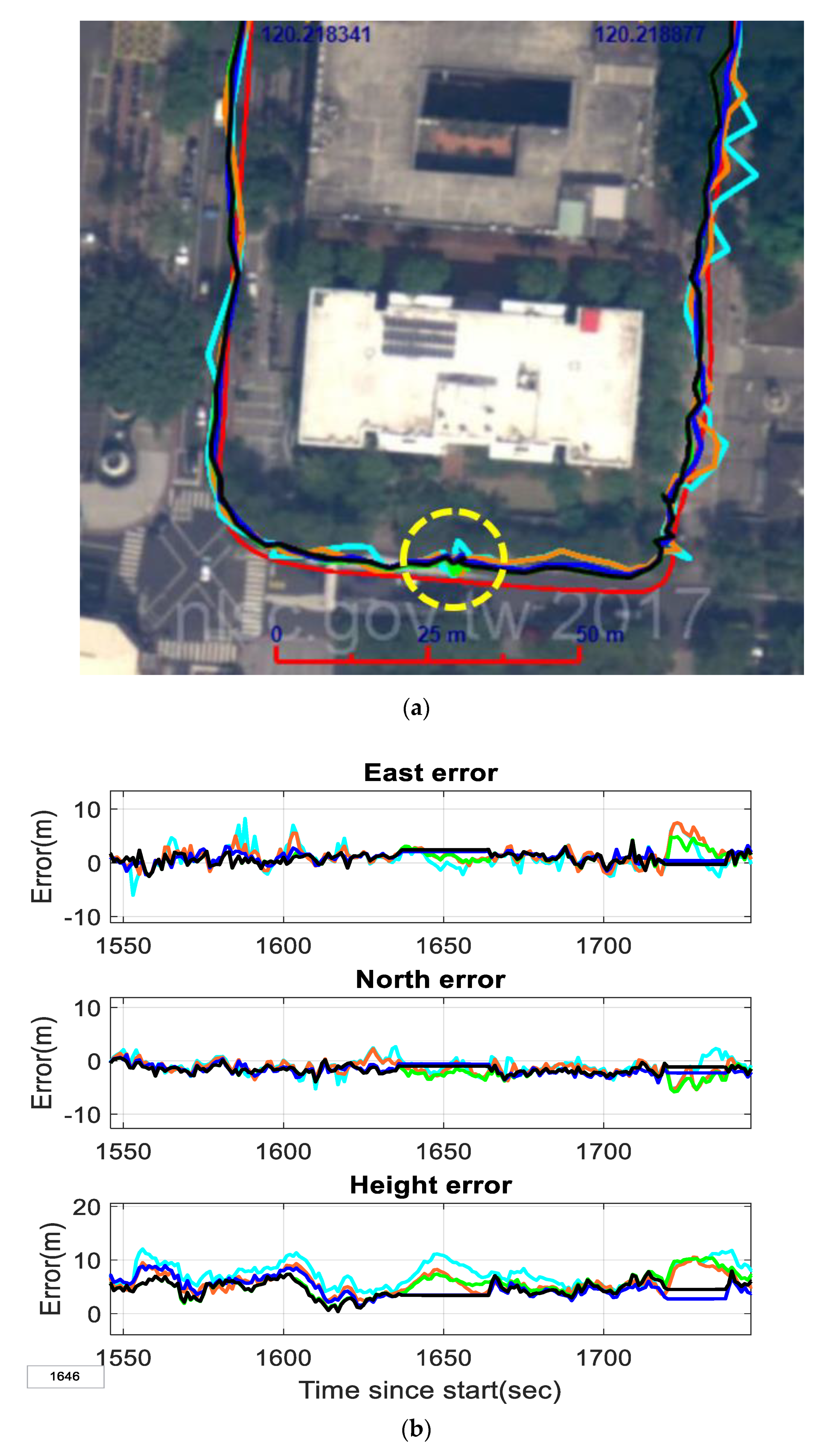
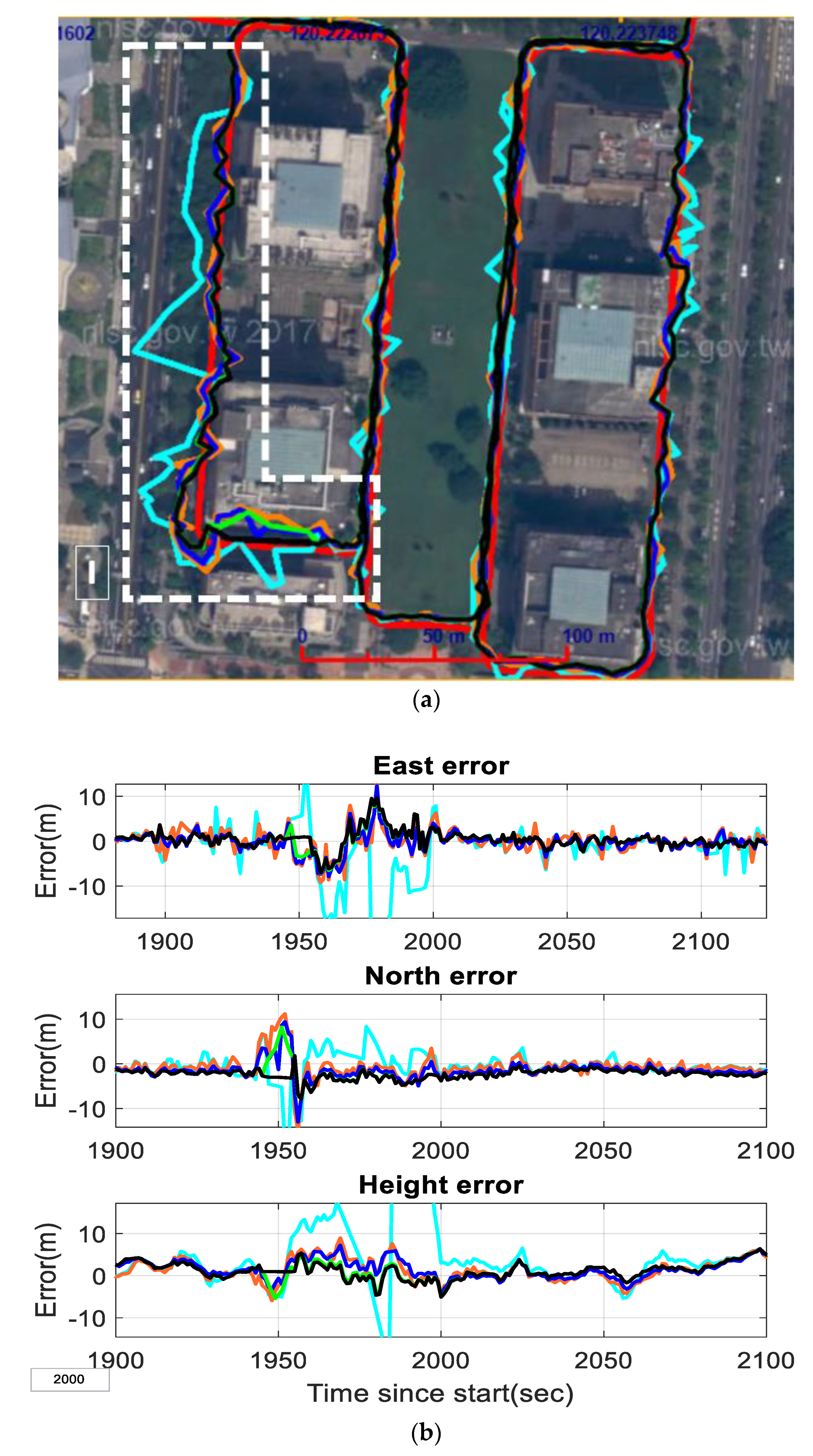
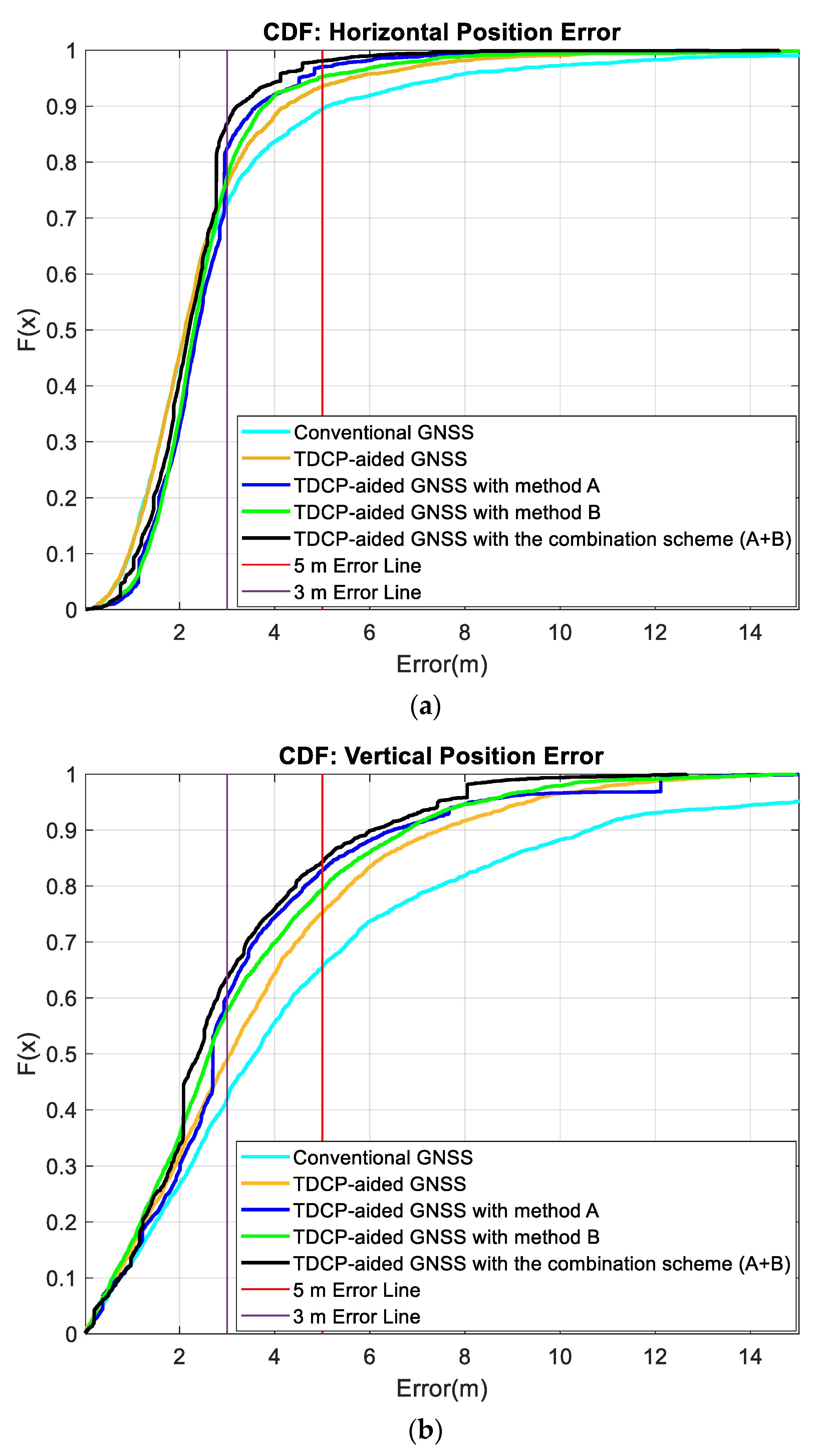
4. Results and Discussion
4.1. Performance Analysis of TDCP-Aided GNSS
4.2. Performance Analysis of TDCP-Aided GNSS with Method A
4.3. Performance Analysis of TDCP-Aided GNSS with Method B
4.4. Performance Analysis of TDCP-Aided GNSS with Both Methods
5. Conclusions
Author Contributions
Funding
Acknowledgments
Conflicts of Interest
References
- Zhou, Z.; Li, B. Optimal Doppler-aided smoothing strategy for GNSS navigation. GPS Solut. 2017, 21, 197–210. [Google Scholar] [CrossRef]
- Kuusniemi, H.; Lachapelle, G.; Takala, J.H. Position and velocity reliability testing in degraded GPS signal environments. GPS Solut. 2017, 8, 226–237. [Google Scholar] [CrossRef]
- Groves, P.D. GNSS: User Equipment Processing and Errors. In Principles of GNSS, Inertial, and Multisensor Integrated Navigation Systems, 2nd ed.; Artech House: Norwood, MA, USA, 2015; pp. 401–407. [Google Scholar]
- Groves, P.D.; Jiang, Z.; Rudi, M.; Strode, P. A Portfolio Approach to NLOS and Multipath Mitigation in Dense Urban Areas; The Institute of Navigation: Manassas, VA, USA, 2013. [Google Scholar]
- Ford, T.J.; Hamilton, J. A new positioning filter: Phase smoothing in the position domain. Navigation 2003, 50, 65–78. [Google Scholar] [CrossRef]
- Lee, H.K.; Rizos, C.; Jee, G.I. Position domain filtering and range domain filtering for carrier-smoothed-code DGNSS: An analytical comparison. IEE Proc.-Radar Sonar Navig. 2005, 152, 271–276. [Google Scholar] [CrossRef]
- Soon, B.K.; Scheding, S.; Lee, H.K.; Lee, H.K.; Durrant-Whyte, H. An approach to aid INS using time-differenced GPS carrier phase (TDCP) measurements. GPS Solut. 2008, 12, 261–271. [Google Scholar] [CrossRef]
- Hsu, L.T. Analysis and modeling GPS NLOS effect in highly urbanized area. GPS Solut. 2018, 22, 7. [Google Scholar] [CrossRef]
- Braasch, M.S. Multipath Effects. In Global positioning System: Theory and Applications Volume I; Parkinson, B.W., Spilker, J.J., Jr., Eds.; AIAA: Washington, DC, USA, 1996; pp. 547–568. [Google Scholar]
- Leisten, O.; Knobe, V. Optimizing small antennas for body-loading applications. GPS World 2012, 23, 40–44. [Google Scholar]
- Blanch, J.; Walter, T.; Enge, P. Fast multiple fault exclusion with a large number of measurements. In Proceedings of the 2015 International Technical Meeting of The Institute of Navigation, Dana Point, CA, USA, 26–28 January 2015. [Google Scholar]
- Iwase, T.; Suzuki, N.; Watanabe, Y. Estimation and exclusion of multipath range error for robust positioning. GPS Solut. 2013, 17, 53–62. [Google Scholar] [CrossRef]
- Hsu, L.T.; Tokura, H.; Kubo, N.; Gu, Y.; Kamijo, S. Multiple faulty GNSS measurement exclusion based on consistency check in urban canyons. IEEE Sens. J. 2017, 17, 1909–1917. [Google Scholar] [CrossRef]
- Sato, K.; Tateshita, H.; Wakabayashi, Y. Asia Oceania Multi-GNSS Demonstration Campaign. In XXV FIG Congress; GIM International: Kuala Lumpur, Malaysia, 2014. [Google Scholar]
- Gao, H.; Groves, P.D. Environmental context detection for adaptive navigation using GNSS measurements from a smartphone. Navig. J. Inst. Navig. 2018, 65, 99–116. [Google Scholar] [CrossRef]
- Castaldo, G.; Angrisano, A.; Gaglione, S.; Troisi, S. P-RANSAC: An integrity monitoring approach for GNSS signal degraded scenario. Int. J. Navig. Obs. 2014, 2014, 1–11. [Google Scholar] [CrossRef]
- Wieser, A.; Brunner, F.K. Short static GPS sessions: Robust estimation results. GPS Solut. 2002, 5, 70–79. [Google Scholar] [CrossRef]
- Gaglione, S.; Innac, A.; Carbone, S.P.; Troisi, S.; Angrisano, A. Robust estimation methods applied to GPS in harsh environments. In Proceedings of the 2017 IEEE European Navigation Conference (ENC), Lausanne, Switzerland, 9–12 May 2017; pp. 14–25. [Google Scholar]
- Gaglione, S.; Angrisano, A.; Crocetto, N. Robust Kalman Filter applied to GNSS positioning in harsh environment. In Proceedings of the 2019 IEEE European Navigation Conference (ENC), Warsaw, Poland, 9–12 April 2019; pp. 1–6. [Google Scholar]
- Groves, P.D.; Jiang, Z.; Wang, L.; Ziebart, M.K. Intelligent urban positioning using multi-constellation GNSS with 3D mapping and NLOS signal detection. In Proceedings of the ION ITM, Nashville, TN, USA, 17–21 September 2012; pp. 458–472. [Google Scholar]
- Ziedan, N.I. Urban positioning accuracy enhancement utilizing 3D buildings model and accelerated ray tracing algorithm. In Proceedings of the 30th International Technical Meeting of the Satellite Division of the Institute of Navigation (ION GNSS+), Portland, OR, USA, 25–29 September 2017. [Google Scholar]
- Hsu, L.T.; Gu, Y.; Kamijo, S. NLOS correction/exclusion for GNSS measurement using RAIM and city building models. Sensors 2015, 15, 17329–17349. [Google Scholar] [CrossRef] [PubMed]
- Wang, L.; Groves, P.D.; Ziebart, M.K. Smartphone shadow matching for better cross-street GNSS positioning in urban environments. J. Navig. 2015, 68, 411–433. [Google Scholar] [CrossRef]
- Peyraud, S.; Bétaille, D.; Renault, S.; Ortiz, M.; Mougel, F.; Meizel, D.; Peyret, F. About non-line-of-sight satellite detection and exclusion in a 3D map-aided localization algorithm. Sensors 2013, 13, 829–847. [Google Scholar] [CrossRef]
- Ng, H.-F.; Zhang, G.; Hsu, L.-T. A Computation Effective Range-based 3D Mapping Aided GNSS using Skymask. J. Navig. 2020, 1, 1–21. [Google Scholar] [CrossRef]
- Wen, W.; Zhang, G.; Hsu, L.T. Correcting NLOS by 3D LiDAR and Building Height to improve GNSS Single Point Positioning. Navigation 2019, 66, 705–718. [Google Scholar] [CrossRef]
- Gao, Z.; Shen, W.; Zhang, H.; Niu, X.; Ge, M. Real-time kinematic positioning of INS tightly aided multi-GNSS ionospheric constrained PPP. Sci. Rep. 2016, 6, 1–16. [Google Scholar] [CrossRef]
- El-Sheimy, N. The Development of VISAT: A Mobile Survey System for GIS Applications; University of Calgary: Calgary, AB, Canada, 2016. [Google Scholar]
- Shin, E.H. Accuarcy Improvement of Low Cost INS/GPS for Land Applications. Graduate Studies; University of Calgary: Calgary, AB, Canada, 2001. [Google Scholar]
- Sharaf, R.; Noureldin, A.; Osman, A.; El-Sheimy, N. Online INS/GPS integration with a radial basis function neural network. IEEE Aerosp. Electron. Syst. Mag. 2005, 20, 8–14. [Google Scholar] [CrossRef]
- El-Sheimy, N.; Youssef, A. Inertial sensors technologies for navigation applications: State of the art and future trends. Satell. Navig. 2020, 1, 2. [Google Scholar] [CrossRef]
- Shin, E.H. Estimation Techniques for Low-Cost Inertial Navigation. Ph.D. Thesis, University of Calgary, Calgary, Alberta, Canada, May 2005. [Google Scholar]
- El-Sheimy, N.; Hou, H.; Niu, X. Analysis and modeling of inertial sensors using Allan variance. IEEE Trans. Instrum. Meas. 2007, 57, 140–149. [Google Scholar] [CrossRef]
- El-Sheimy, N.; Chiang, K.W.; Noureldin, A. The utilization of artificial neural networks for multisensor system integration in navigation and positioning instruments. IEEE Trans. Instrum. Meas. 2006, 55, 1606–1615. [Google Scholar] [CrossRef]
- Lahrech, A.; Boucher, C.; Noyer, J.C. Fusion of GPS and odometer measurements for map-based vehicle navigation. In Proceedings of the 2004 IEEE International Conference on Industrial Technology (ICIT’04), Hammamet, Tunisia, 8–10 December 2004; Volume 2, pp. 944–948. [Google Scholar]
- Seo, J.; Lee, H.K.; Lee, J.G.; Park, C.G. Lever arm compensation for GPS/INS/odometer integrated system. Int. J. Control Autom. Syst. 2006, 4, 247–254. [Google Scholar]
- Mosavi, M.R.; Azad, M.S.; EmamGholipour, I. Position estimation in single-frequency GPS receivers using Kalman filter with pseudo-range and carrier phase measurements. Wirel. Pers. Commun. 2013, 72, 2563–2576. [Google Scholar] [CrossRef]
- Misra, P.; Enge, P. Global Positioning System: Signals, Measurements and Performance, 2nd ed.; Ganga-Jamuna Press: Lincoln, MA, USA, 2006; Volume 206. [Google Scholar]
- van Graas, F.; Soloviev, A. Precise Velocity Estimation Using a Stand-Alone GPS Receiver. Navigation 2004, 51, 283–292. [Google Scholar] [CrossRef]
- Serrano, L.; Kim, D.; Langley, R.B.; Itani, K.; Ueno, M. A GPS velocity sensor: How accurate can it be?—A first look. In Proceedings of the ION NTM, San Diego, CA, USA, 26–28 January 2004; pp. 875–885. [Google Scholar]
- Wendel, J.; Meister, O.; Monikes, R.; Trommer, G.F. Time-differenced carrier phase measurements for tightly coupled GPS/INS integration. In Proceedings of the 2006 IEEE/ION Position, Location, and Navigation Symposium, San Diego, CA, USA, 25–27 April 2006; pp. 54–60. [Google Scholar]
- Ding, W.; Wang, J. Precise velocity estimation with a stand-alone GPS receiver. J. Navig. 2001, 64, 311–325. [Google Scholar] [CrossRef]
- Freda, P.; Angrisano, A.; Gaglione, S.; Troisi, S. Time-differenced carrier phases technique for precise GNSS velocity estimation. GPS Solut. 2015, 19, 335–341. [Google Scholar] [CrossRef]
- Aftatah, M.; Lahrech, A.; Abounada, A. Fusion of GPS/INS/Odometer measurements for land vehicle navigation with GPS outage. In Proceedings of the 2016 IEEE 2nd International Conference on Cloud Computing Technologies and Applications (CloudTech), Marrakech, Morocco, 24–26 May 2016; pp. 48–55. [Google Scholar]
- Georgy, J.; Noureldin, A.; Bayoumi, M. Mixture particle filter for low cost INS/odometer/GPS integration in land vehicles. In Proceedings of the VTC Spring 2009-IEEE 69th Vehicular Technology Conference, Barcelona, Spain, 26–29 April 2009; pp. 1–5. [Google Scholar]
- Knight, N.L.; Wang, J. A comparison of outlier detection procedures and robust estimation methods in GPS positioning. J. Navig. 2009, 62, 699–709. [Google Scholar] [CrossRef]
- Stephenson, S. Automotive Applications of High Precision GNSS. Ph.D. Thesis, University of Nottingham, Nottingham, UK, June 2016. [Google Scholar]
- Basnayake, C.; Williams, T.; Alves, P.; Lachapelle, G. Can GNSS Drive V2X? GPS World 2010, 21, 35–43. [Google Scholar]
- National Highway Traffic Safety Administration and Department of Transportation. Federal Motor Vehicle Safety Standards; V2V Communications, Docket No. NHTSA–2016–0126, RIN 2127–AL55; Federal Register: Washington, DC, USA, 2017.
- Reid, T.G.; Houts, S.E.; Cammarata, R.; Mills, G.; Agarwal, S.; Vora, A.; Pandey, G. Localization requirements for autonomous vehicles. arXiv 2019, arXiv:1906.01061. [Google Scholar] [CrossRef]


| Accelerometer | Gyroscope | |
|---|---|---|
| Bias instability | ||
| Random walk noise |
| Unit: m/s | Overall 1 | Straight 2 | Turning 3 |
|---|---|---|---|
| Mean | 0.053 | 0.068 | 0.116 |
| Max | 1.282 | 0.929 | 1.043 |
| STD | 0.141 | 0.132 | 0.205 |
| RMSE | 0.151 | 0.148 | 0.235 |
| Unit: m | 3D | ||||
|---|---|---|---|---|---|
| Conventional GNSS | TDCP-Aided GNSS | TDCP-Aided GNSS + Method A | TDCP-Aided GNSS + Method B | TDCP-Aided GNSS + Method A Method B | |
| Mean | 5.84 | 4.75 | 4.16 | 4.80 | 3.65 |
| Max | 37.24 | 19.42 | 12.45 | 15.00 | 8.88 |
| RMSE | 8.35 | 5.68 | 4.87 | 5.57 | 4.06 |
| RMSE Improvement | - | 32.0% | 41.7% | 33.3% | 51.4% |
| Unit: m | Forward/Lateral | ||||
|---|---|---|---|---|---|
| Conventional GNSS | TDCP-Aided GNSS | TDCP-Aided GNSS + Method A | TDCP-Aided GNSS + Method B | TDCP-Aided GNSS + Method A Method B | |
| Mean | −0.41/−0.47 | 0.39/−0.54 | −0.49/−0.61 | −0.47/−0.55 | −0.37/−0.49 |
| Max | 25.95/17.21 | 14.92/10.05 | 12.6/9.30 | 15.86/10.60 | 10.75/12.75 |
| RMSE | 2.98/2.47 | 2.21/2.07 | 1.87/2.10 | 2.09/2.16 | 1.63/1.95 |
| RMSE Improvement | - | 25.8%/16.2% | 37.2%/15.0% | 29.9%/12.6% | 45.3%/21.1% |
| Satellite 1 | Range Measurement 2 | True Range | Range Error 3 | Residual 4 | Scale 4 |
|---|---|---|---|---|---|
| G14 | 22,492,867.56 | 22,492,830.40 | 37.16 | 26.96 | 2.77 |
| G25 | 20,580,188.56 | 20,580,187.61 | 0.95 | 3.78 | 1.00 |
| G31 | 21,729,429.25 | 21,729,415.49 | 13.76 | −1.26 | 1.00 |
| G32 | 21,213,735.12 | 21,213,711.48 | 23.65 | 18.87 | 1.94 |
| C6 | 35,967,621.88 | 35,967,615.37 | 6.51 | 5.39 | 1.00 |
| C7 | 36,142,589.49 | 36,142,586.11 | 3.38 | −3.68 | 1.00 |
| C9 | 36,559,641.75 | 36,559,610.28 | 31.47 | 24.93 | 2.56 |
| C10 | 37,151,565.47 | 37,151,546.00 | 19.47 | 7.93 | 1.00 |
| Unit: m | Horizontal/Vertical | ||||
|---|---|---|---|---|---|
| Conventional GNSS | TDCP-Aided GNSS | TDCP-Aided GNSS + Method A | TDCP-Aided GNSS + Method B | TDCP-Aided GNSS + Method A Method B | |
| Mean | 2.83/4.78 | 2.47/3.41 | 2.50/3.17 | 2.57/3.05 | 2.28/2.88 |
| Max | 27.66/34.18 | 15.20/14.95 | 13.15/17.47 | 16.82/14.97 | 14.61/12.67 |
| RMSE | 3.87/7.20 | 3.01/4.55 | 2.79/4.16 | 2.98/4.11 | 2.51/3.63 |
| RMSE Improvement | - | 22.3%/36.8% | 28.0%/42.0% | 23.0%/42.9% | 35.1%/49.6% |
| Which Road1(3 m)2 | 72.0%/42.4% | 75.4%/49.3% | 81.8%/60.4% | 76.7%/58.1% | 86.1%/63.9% |
| Which Road1(5 m)2 | 89.5%/65.8% | 93.5%/75.4% | 96.3%/82.9% | 94.4%/79.5% | 97.3%/84.4% |
© 2020 by the authors. Licensee MDPI, Basel, Switzerland. This article is an open access article distributed under the terms and conditions of the Creative Commons Attribution (CC BY) license (http://creativecommons.org/licenses/by/4.0/).
Share and Cite
Chiang, K.-W.; Li, Y.-H.; Hsu, L.-T.; Chu, F.-Y. The Design a TDCP-Smoothed GNSS/Odometer Integration Scheme with Vehicular-Motion Constraint and Robust Regression. Remote Sens. 2020, 12, 2550. https://doi.org/10.3390/rs12162550
Chiang K-W, Li Y-H, Hsu L-T, Chu F-Y. The Design a TDCP-Smoothed GNSS/Odometer Integration Scheme with Vehicular-Motion Constraint and Robust Regression. Remote Sensing. 2020; 12(16):2550. https://doi.org/10.3390/rs12162550
Chicago/Turabian StyleChiang, Kai-Wei, Yu-Hua Li, Li-Ta Hsu, and Feng-Yu Chu. 2020. "The Design a TDCP-Smoothed GNSS/Odometer Integration Scheme with Vehicular-Motion Constraint and Robust Regression" Remote Sensing 12, no. 16: 2550. https://doi.org/10.3390/rs12162550
APA StyleChiang, K.-W., Li, Y.-H., Hsu, L.-T., & Chu, F.-Y. (2020). The Design a TDCP-Smoothed GNSS/Odometer Integration Scheme with Vehicular-Motion Constraint and Robust Regression. Remote Sensing, 12(16), 2550. https://doi.org/10.3390/rs12162550