Article

Remote Sensing Estimation of Regional NO2 via Space-Time Neural Networks

1
School of Resource and Environmental Sciences, Wuhan University, Wuhan 430079, China
2
School of Geodesy and Geomatics, Wuhan University, Wuhan 430079, China
3
Key Laboratory of Geospace Environment and Geodesy, Ministry of Education, Wuhan University, Wuhan 430079, China
*
Author to whom correspondence should be addressed.
Remote Sens. 2020, 12(16), 2514; https://doi.org/10.3390/rs12162514
Submission received: 26 June 2020 / Revised: 29 July 2020 / Accepted: 31 July 2020 / Published: 5 August 2020
(This article belongs to the Section Environmental Remote Sensing)

Abstract

:
Nitrogen dioxide (NO2) is an essential air pollutant related to adverse health effects. A space-time neural network model is developed for the estimation of ground-level NO2 in this study by integrating ground NO2 station measurements, satellite NO2 products, simulation data, and other auxiliary data. Specifically, a geographically and temporally weighted generalized regression neural network (GTW-GRNN) model is used with the advantage to consider the spatiotemporal variations of the relationship between NO2 and influencing factors in a nonlinear neural network framework. The case study across the Wuhan urban agglomeration (WUA), China, indicates that the GTW-GRNN model outperforms the widely used geographically and temporally weighted regression (GTWR), with the site-based cross-validation R2 value increasing by 0.08 (from 0.61 to 0.69). Besides, the comparison between the GTW-GRNN and original global GRNN models shows that considering the spatiotemporal variations in GRNN modeling can boost estimation accuracy. All these results demonstrate that the GTW-GRNN based NO2 estimation framework will be of great use for remote sensing of ground-level NO2 concentrations.

Graphical Abstract

1. Introduction

Nitrogen dioxide (NO2) is an essential air pollutant and has been reported to be associated with adverse effects on human health by epidemiological studies [1,2,3,4]. Faustini et al. [5] have found that per 10 μg/m3 of NO2 causes a 4% increase in mortality. Besides, NO2 plays a vital role in the formation of acid rain and disorders greenhouse gas and ozone levels that can affect the global climate [6]. As a result, it is an urgent need to monitor NO2 concentrations. Recently, remote sensing retrieval of ground NO2 concentrations has aroused wide attention [7,8,9,10,11,12,13], for providing broader spatiotemporal coverages beyond ground monitoring stations, which act as the primary approach for the monitoring of NO2 all the time.
For the remote sensing retrieval of ground NO2, a common way is to construct the statistical relationship between satellite troposphere NO2 data and ground NO2 measurements, with the theoretical foundation that the close association exists in them [14,15]. Many satellite sensors can provide troposphere NO2 products, such as the Ozone Monitoring Instrument (OMI) [16], the Global Ozone Monitoring Experiment (GOME) [17], and the TROPOspheric Monitoring Instrument (TROPOMI) [18,19]. Thanks to so many satellite observations for NO2 information, the daily (seasonal or annual) ground NO2 concentrations can be effectively obtained via a statistical model from regional to global scales. For instance, Qin et al. [15] estimated ground NO2 concentrations from OMI data over east-central China using the relatively advanced geographically and temporally weighted regression (GTWR) statistical model.
In recent years, machine learning models have achieved widespread applications in remote sensing retrieval of ground NO2 concentrations, which can be attributed to their advantages in describing the nonlinear relationship between ground NO2 and influencing factors. These machine learning models, including random forest [9,20], neural network (NN) [21], Bayesian maximum entropy [22], extreme gradient boosting [23], and so on, have generally reported some advantages in estimation accuracy over traditional statistical models and played a critical role in remote sensing retrieval of ground NO2 concentrations.
However, the current machine learning models for ground NO2 estimation usually perform with an assumption that the relationship between NO2 and influencing factors does not vary in the whole study domain and period. In other words, the machine learning modes are based on a global modeling technique, and thus fail to consider the spatiotemporal variations of the relationship between NO2 and influencing factors.
Therefore, this research aims to estimate ground NO2 concentrations using a space-time neural network (STNN) model, which can allow for the spatiotemporal variations. The TROPOMI NO2 product, the Goddard Earth Observing System Data Assimilation System GEOS-5 Forward Processing (GEOS 5-FP) simulated NO2 related variable and meteorological data, and other auxiliary data are used as input for the STNN model, and the STNN model is trained with ground NO2 station measurements. It is noteworthy that the new-generation TROPOMI sensor holds great potentials to assess NO2 concentration [24], which helps capture detailed NO2 distribution in this research. Through the above process, the STNN model is expected to fit the nonlinear NO2 estimation function effectively and can be used to estimate ground NO2 from remote sensing data.

2. Study Area and Materials
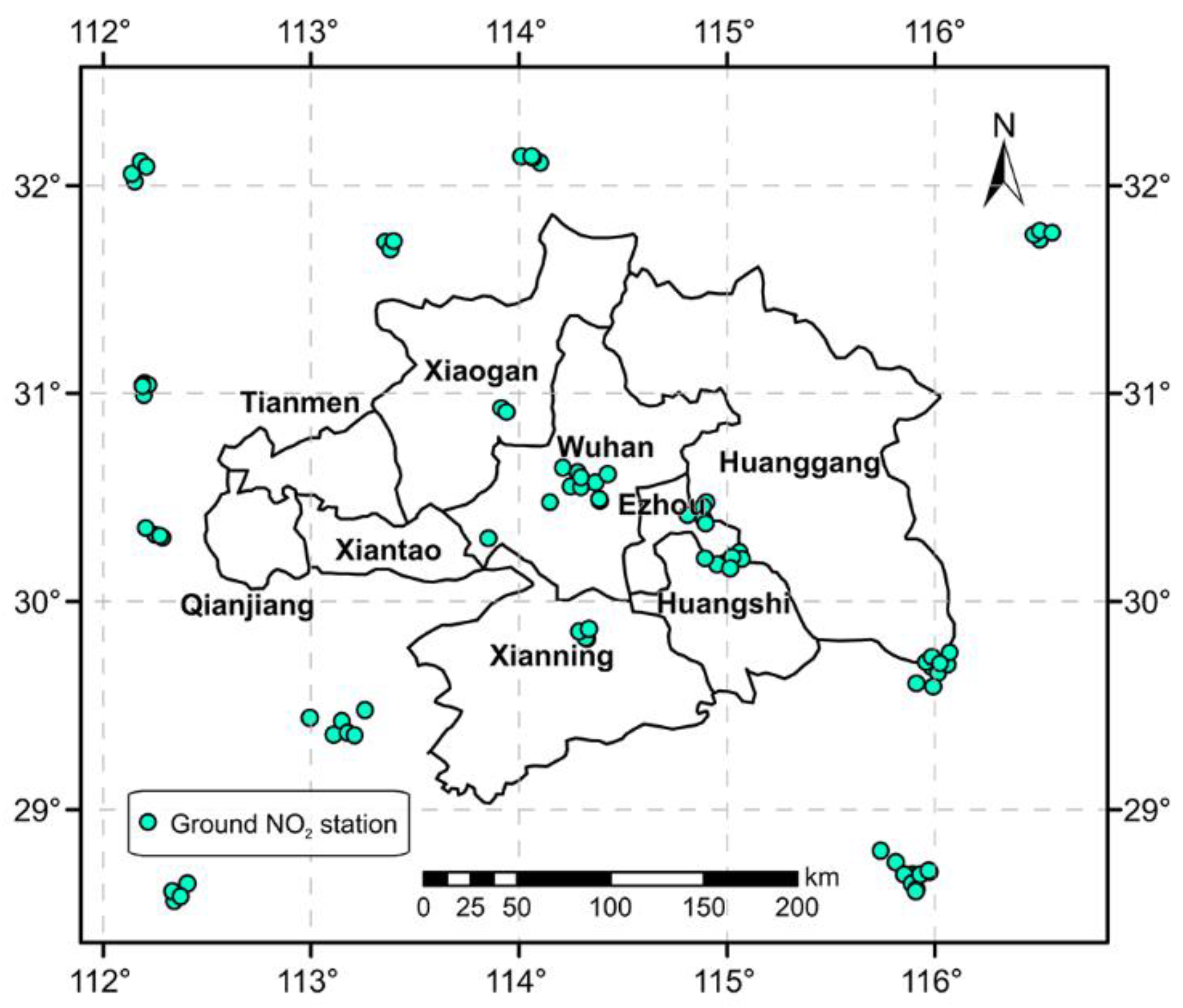
2.1. Study Area

The Wuhan urban agglomeration (WUA) region was selected as the study area, which is displayed in Figure 1. The WUA region is situated in the central part of China. It consists of the Wuhan city and eight surrounding cities, i.e., Ezhou, Huangshi, Xianning, Xiaogan, Huanggang, Tianmen, Qianjiang, and Xiantao [25]. In recent years, the WUA region is suffering from a severe air pollution problem, due to the rapid development of the economy [26,27]. Hence, it is of considerable significance to dynamically monitor ground NO2 concentrations in the WUA region.
The NO2 monitoring stations in the WUA region are used for analysis, as shown in Figure 1. Also, we further include the monitoring stations outside the WUA region to make full use of the ground NO2 measurements, which are located in the range of 28.4°~32.3° N and 112.0°~116.7° E. A total of 84 NO2 monitoring stations were collected in this research.

2.2. Materials

2.2.1. NO2 Station Measurements

The hourly NO2 data measured from 84 monitoring stations (see Figure 1) were obtained from http://106.37.208.233:20035/. In this research, the data during the period of 1 January 2019 to 31 December 2019 were used. The measurement method for ground NO2 concentration is determined in the Chinese National Ambient Air Quality Standard (GB 3095-2012), which has high standards of calibration and quality control. In this research, the hourly NO2 data corresponding to the overpass time of the satellite was extracted for modeling.

2.2.2. TROPOMI Tropospheric NO2 Data

The Sentinel-5 Precursor (S5P) satellite can provide daily global products of trace gases and aerosols, which are of great use for air quality monitoring. The sensor onboard S5P satellite is the TROPOMI [18,28], which covers the spectral bands of the shortwave infrared, the near-infrared, the visible, and the ultraviolet. These spectral bands of observations make the TROPOMI sensor able to monitor ozone (O3), NO2, sulfur dioxide (SO2), and aerosols, etc.
The TROPOMI tropospheric NO2 product was retrieved based on the Dutch OMI NO2 data approach and European “Quality Assurance for Essential Climate Variables” project (QA4ECV) processing systems [29]. The TROPOMI tropospheric NO2 products were available at https://disc.gsfc.nasa.gov/datasets?keywords=Sentinel-5P. A previous study has revealed the high consistency between TROPOMI NO2 and widely-used OMI NO2 data over China [24]. In our study, the data field of “nitrogendioxide_tropospheric_column” was extracted, and this product was resampled to 0.05° × 0.05°.

2.2.3. GEOS 5-FP NO2 Related Variable and Meteorological Conditions

We introduced two main types of GEOS 5-FP data [30] into the ground NO2 estimation modeling. The first is NO2 related variable, i.e., nitric acid surface mass concentration (denoted as NOsim). The other is meteorological conditions, i.e., surface pressure, 10-m specific humidity, 2-m air temperature, 10-m eastward wind, 10-m northward wind, planetary boundary layer height, and evaporation from turbulence. The former type of data is recognized as a primary factor, and the latter is incorporated as the covariates for the ground NO2 estimation modeling. The resolution of the above data is 0.25° × 0.3125°, and the additional information can be found at https://fluid.nccs.nasa.gov/weather/.

2.2.4. Other Auxiliary Data

In addition, Moderate-resolution Imaging Spectroradiometer (MODIS) normalized difference vegetation index (NDVI) data (identifier: MYD13C1) is used as the land cover-related covariate in the ground NO2 estimation modeling. The NDVI data can be obtained at https://ladsweb.modaps.eosdis.nasa.gov. Also, the terrain-related variable, i.e., digital elevation model (DEM), is adopted, and its details can refer to Danielson et al. [31].

3. Methodology

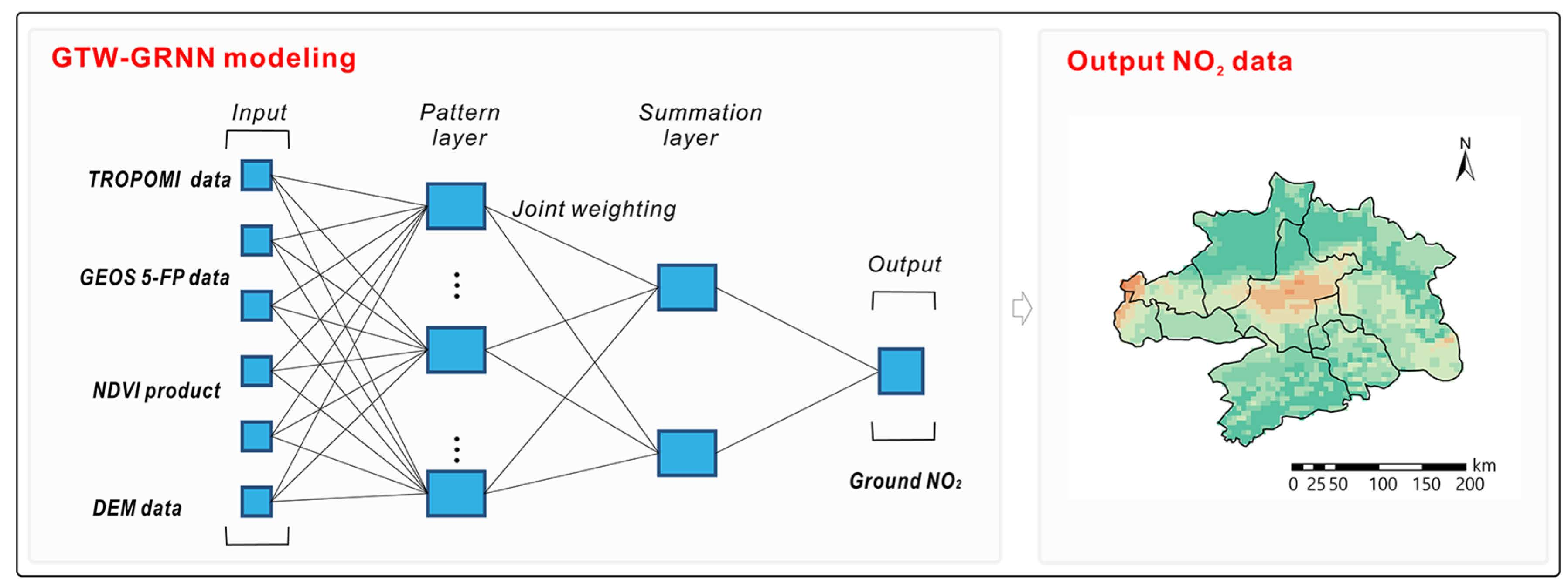
3.1. The STNN Model for NO2 Estimation

The NN models have been applied for satellite-based NO2 estimation, and they usually establish a global relationship between ground NO2 and influencing factors, i.e., N O 2 = f ( N O 2 , s a t , X ) , where NO2,sat means satellite observations of NO2 and X refers to other influencing factors, such as meteorological data, NDVI, etc. However, global NN modeling fails to allow for the spatiotemporal variations of the relationship between ground NO2 and influencing factors. To address this issue, an STNN model is adopted in this research, whose general structure is shown as follows.
N O 2 = f ( x j , y j , t j ) ( N O 2 , s a t , N O s i m , M e t e o r o l o g y , N D V I , D E M )
where NOsim means the GEOS 5-FP simulated NO2 related variable, Meteorology is the GEOS 5-FP meteorological data. The details of the input variables can be found in Section 2.2. f ( x j , y j , t j ) refers to the location-time-specific NN model, which varies in space and time to cope with the spatiotemporal variations. ( x j , y j ) denotes the spatial coordinate and t j   stands for the time of grid cell j.
In this research, the generalized regression neural network (GRNN) [32,33] model is utilized for mapping the relationship between ground NO2 and influencing factors, that is, f ( x j , y j , t j ) is represented by the GRNN model. Figure 2 shows the schematic of the space-time varying GRNN model for ground NO2 estimation, which is denoted as geographically and temporally weighted GRNN (GTW-GRNN). The GTW-GRNN model is separately constructed for each location and time, and the modeling process contains two main steps, i.e., spatiotemporal weighting and GRNN modeling, which are simply described as follows. For details, please refer to our previous study [34].
For the spatiotemporal weighting, the widely used Gaussian function is applied to describe the contribution of each sample to the estimation of NO2 for grid cell j. To be specific, the weight of sample k can be depicted as Equation (2):
w k = e x p ( d s k 2 + λ d t k 2 h S T 2 )
where dsk and dtk respectively stand for the spatial and the temporal distance of sample k to grid cell j. λ is a factor to counterweigh the spatial distance and temporal distance. hST is considered as spatiotemporal bandwidth in the spatiotemporal weighting scheme [35,36].
For the GRNN modeling, the critical issue is how to incorporate spatiotemporal weighting into the GRNN model (i.e., establishing the GTW-GRNN model). Compared with the original GRNN model, the GTW-GRNN model does not change the neural network structure, but it introduces the spatiotemporal weighting into the weights between the pattern layer and the summation layer. Thus, a joint weighting of spatiotemporal weighting and GRNN weighting is used for estimating ground NO2 concentrations. Additional details about GTW-GRNN modeling can be found in our previous study [34].

3.2. The Procedure of STNN-Based NO2 Estimation

Figure 3 shows the procedure of satellite-based NO2 estimation using the GTW-GRNN model, which can be divided into three main steps: (1) data pre-processing and matching, (2) GTW-GRNN modeling and validation, and (3) spatiotemporal mapping of ground NO2.
(1) Data pre-processing and matching. The variables mentioned in Section 2.2. are firstly extracted from the original datasets to form the input dataset. During this process, all the data are converted to the WGS84 geographic coordinate system and resampled to 0.05° in accordance with the spatial resolution of TROPOMI observation. Subsequently, the values of TROPOMI observation, GEOS 5-FP data, and other auxiliary data are extracted according to the locations of NO2 monitoring stations. Meanwhile, multiple NO2 station measurements are averaged in each 0.05° grid cell.
(2) GTW-GRNN modeling and validation. For each location and time, a GTW-GRNN model is established and trained with local samples (see Section 3.1). Then a cross-validation (CV) technique [37] is adopted to evaluate model performance and to be specific, the site-based CV [38] is utilized for the model validation in this research. For the site-based CV, all the grid cells with NO2 monitoring stations are partitioned into ten folds randomly and averagely, where one fold is used as the validation set, and nine folds are adopted for model fitting. This process will be repeated ten times until each fold has been used for model validation. At the same time, the following statistical indicators are calculated for accuracy evaluation: root-mean-square error (RMSE, unit: μg/m3) and coefficient of determination (R2, unitless).
(3) Spatiotemporal mapping of ground NO2. After the validation process, the GTW-GRNN model can be utilized for the mapping of ground NO2 concentrations. For each grid cell in the spatiotemporal dimension, the data samples are inputted into the GTW-GRNN model, and the output NO2 value can be obtained. Thus, the spatiotemporal distribution of NO2 concentrations can be mapped through the above processes.

4. Results and Analysis

To fully assess the performance of the GTW-GRNN model, it was compared to the global GRNN model and the GTWR model, both of them have been widely used in remote sensing estimation modeling of air quality [39,40,41]. The selection for these two models is subject to the following reasons: (1) the global GRNN does not consider the spatial and temporal variations of the relationship between NO2 and influencing factors, the comparison between the global GRNN and GTW-GRNN models can thus reveal the function of considering the spatiotemporal variations in GRNN. (2) the GTWR and GTW-GRNN models share similar modeling strategies, whereas the former is based on a linear assumption, and the latter uses the nonlinear NN modeling technique.

4.1. Overall Performance of the Models

Figure 4 shows the site-based CV performance of the GTWR, global GRNN, and GTW-GRNN models. As can be observed from Figure 4, the GTWR model shows a relatively poor performance, with RMSE and R2 values being 9.25 μg/m3 and 0.61, respectively. Then a slightly better performance is achieved by the global GRNN model, whose CV RMSE and R2 values are 9.14 μg/m3 and 0.62, respectively. The GTWR model can allow for the spatiotemporal variations of the association between ground NO2 and influencing factors, whereas it is based on a linear assumption. On the contrary, the global GRNN model can fit the nonlinear relationship, whereas it fails to consider the spatiotemporal variations. Comparing the GTWR and global GRNN models, the global GRNN model shows a slight advantage in such a relatively small WUA region. Thanks to the ability to simultaneously cope with nonlinear fitting and spatiotemporal variations, the GTW-GRNN model performs the best for ground NO2 estimation, with CV RMSE and R2 values of 8.29 μg/m3 and 0.69, respectively. In addition, the GTW-GRNN model shows the lightest degree of underestimation/overestimation among the three models, which has a CV slope value of 0.75. The underestimation/overestimation is a common phenomenon in remote sensing of air quality modeling [42], and the possible reasons could be that the station measurements cannot represent the grid cell. The lack of high values for model training is also likely to result in that phenomenon. In summary, all the results demonstrate that the GTW-GRNN model is advantageous for the remote sensing retrieval of ground NO2 concentrations.

4.2. Model Performance for Each Season

The seasonal performance of the models is shown in Table 1. Firstly, the GTW-GRNN model has obtained the best performance among the three models, with R2s being 0.55, 0.34, 0.61, and 0.64 for spring (March to May), summer (June to August), autumn (September to November), and winter (December, January, and February), respectively. Meanwhile, the seasonal R2 values for the global GRNN (GTWR) model are 0.50 (0.40), 0.25 (0.18), 0.56 (0.58), and 0.54 (0.56), respectively. Also, from the view of RMSE and slope, the GTW-GRNN model shows some advantages over the other two models for ground NO2 estimation for all the four seasons. Specifically, the RMSE values decrease from 10.06 μg/m3 to 8.57 μg/m3 (spring), from 7.12 μg/m3 to 6.28 μg/m3 (summer), from 7.99 μg/m3 to 7.73 μg/m3 (autumn), and from 11.39 μg/m3 to 10.27 μg/m3 (winter), respectively, when comparing the GTW-GRNN model to the GTWR model.
Secondly, large seasonal variations can be found in Table 1, where summer shows the most miserable performance, and autumn and winter report significant increase for model fitting goodness. Taking the GTW-GRNN model as an example, the RMSE, R2, and slope values are 6.28 μg/m3, 0.34, and 0.48, respectively, for summer, whereas the corresponding metric values are 10.27 μg/m3, 0.64, and 0.70, apiece, for winter. A higher slope value generally means a lighter degree of underestimation/overestimation, so the models tend to better estimate NO2 high/low values in winter than in summer. Besides, it should be noted that winter has a higher RMSE value than other seasons. RMSE value is an absolute metric and the high level of NO2 concentrations in winter results in the high RMSE value. The reason for seasonal variations could be related to seasonal differences of NO2 values, formation conditions, etc.

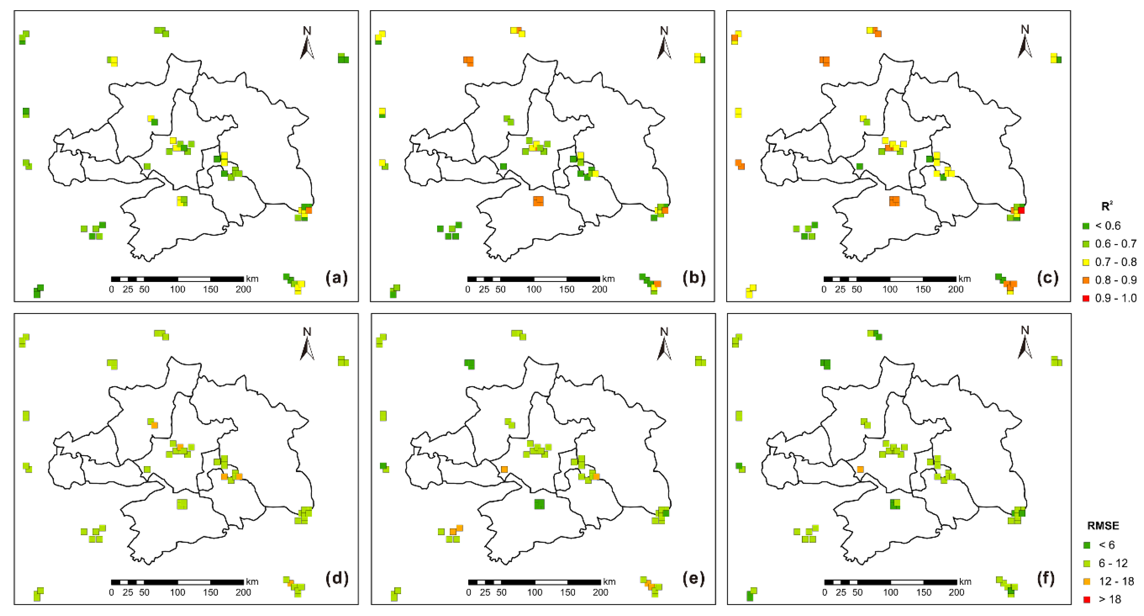
4.3. Model Performance for Each Grid Cell

We also evaluate the model performance for each grid cell, which is shown in Figure 5. Overall, the mean R2 (RMSE) for the GTWR, global GRNN, and GTW-GRNN models are 0.64 (9.08 μg/m3), 0.66 (8.82 μg/m3), and 0.72 (7.95 μg/m3), respectively. Meanwhile, 45, 44, and 53 out of 63 grid cells respectively achieve high R2 values of greater than 0.6 for the GTWR, global GRNN, and GTW-GRNN models. These results indicate that the GTW-GRNN model performs the best, whereas the GTWR is the poorest for the overall performance. Spatially, higher values of R2 are found for GTW-GRNN compared to the GTWR and global GRNN models in Wuhan, Ezhou, and Xianning cities. Accordingly, lower RMSE values for the GTW-GRNN model can be observed in Ezhou city.
On the other hand, the site-based CV is considered as an effective solution to reflect spatial prediction accuracy [38]. As shown in Figure 5c, most of the grid cells can obtain a high R2 value (as mentioned before, 84% grid cells with R2 > 0.6), indicating that the GTW-GRNN predictions show high consistency to ground station measurements. The above results reveal GTW-GRNN modeling is an appropriate approach for satellite-based spatial mapping of ground NO2 concentrations.

5. Discussion

5.1. Mapping Results of Ground NO2 Concentrations

Based on the GTW-GRNN model, the spatial distributions of ground NO2 concentrations are mapped. As shown in Figure 6, four days (1 January 2019, 9 May 2019, 21 August 2019, and 8 October 2019) of mapping results are presented as an example. Overall, the distributions of the remote sensing retrievals of NO2 show an excellent agreement to station measurements for the given four days. Among the four days, 1 January 2019 reports relatively high levels of NO2 concentrations, and 9 May 2019 and 21 August 2019 are cleaner. Spatially, Wuhan is a severe NO2 pollution center, which has the most urbanized degree in the WUA region.
To quantitatively evaluate the consistency between remote sensing retrievals and station measurements, we calculate the RMSE and R2 values, as shown in Table 2. For the whole year, a good agreement is found, with the RMSE and R2 values being 4.55 μg/m3 and 0.91, respectively, indicating that the GTW-GRNN model achieves a good fit for the relationship between ground NO2 and influencing factors. For the above mentioned four days, the R2s are 0.76, 0.75, 0.84, and 0.81, respectively, which confirms the high consistency between remote sensing retrievals and station measurements.

5.2. The Novelty of Incorporating Spatiotemporal Weighting into GRNN

A GTW-GRNN model was applied to estimate ground NO2 concentrations in this research, of which the novelty lies in two main aspects when comparing to the original GRNN model. The first is the GTW-GRNN model uses a local modeling strategy and thus can address the spatiotemporal variations. The other is that a spatiotemporal weighting scheme is introduced to capture the relation of data samples for NO2 estimation. We now compare the GTW-GRNN model with the global GRNN model and the local GRNN model without spatiotemporal weighting, that is, the spatiotemporal weights are all set as 1 in the GTW-GRNN modeling process.
As Table 3 shows, the global GRNN performs the poorest, with CV RMSE and R2 values being 9.25 μg/m3 and 0.61, respectively, for the reason that the global GRNN model cannot address the spatiotemporal variations and estimate ground NO2 concentrations using constant model coefficients. Based on a local modeling strategy, the local GRNN model can consider the spatiotemporal variations, and the ground NO2 is estimated using spatially and temporally varying model coefficients. Thus, the local GRNN model obtains a more advantageous performance, the CV RMSE, R2, and slope values are 8.61 μg/m3, 0.66, and 0.71, respectively. By further incorporating spatiotemporal weighting, the GTW-GRNN model achieves the best performance. These results demonstrate that combining spatiotemporal weighting derived from geographical laws and neural networks can boost the estimation accuracy.

5.3. Impact of Aerosol on Satellite-Based NO2 Modeling

Aerosol optical depth (AOD) has been reported to be closely correlated to NO2, and ul-Haq et al. [43] have revealed that the correlation coefficient between NO2 and AOD is as high as 0.49 over South Asia during 2005–2015. Hence, the AOD data is likely to be useful for the remote sensing retrieval of ground NO2. In this research, the AOD product is not adopted for the following reasons. First, in the remote sensing of air quality field, AOD product has been widely considered as a proxy to estimate ground particulate matter [7,44], and the remote sensing retrieval of ground NO2 usually uses satellite observed NO2 data [8,9,15]. Hence, the selection of satellite data of this work is in line with previous studies. Second, the widely used AOD products (e.g., MODIS AOD) are often missing, whose missing proportion is greater than that of TROPOMI NO2 data. If the AOD product is incorporated, it may introduce more data absence in the ground NO2 estimates. In summary, this work pays more attention to address the spatiotemporal variations in the NO2 neural network estimation framework, so we did not further investigate the influencing factors of NO2. However, considering the high correlation between AOD and NO2, it remains an interesting direction to introduce AOD data in remote sensing retrieval of ground NO2.

5.4. Limitations

There are still some limitations to the remote sensing retrieval of ground NO2 concentrations in this study. Firstly, the missing TROPOMI data results in the incomplete information of remote sensing NO2 retrievals, which may bring limitations for further applications. The data filling for TROPOMI data is not conducted in this research, for the reason that the fundamental purpose of this research is to develop the GTW-GRNN based remote sensing NO2 retrieval framework, the data filling may introduce additional errors. Secondly, the study region focuses on WUA, which is a relatively small area. New challenges and problems will come out for estimating ground NO2 over a broader geographical region. Hence, it remains our further studies to estimate larger scales of NO2 data using the GTW-GRNN based NO2 estimation framework proposed in this research.

6. Conclusions and Future Work

In this study, a GTW-GRNN model was applied to estimate ground NO2 concentrations by integrating ground NO2 station measurements, TROPOMI NO2 products, GEOS 5-FP data, and other auxiliary data. The contribution of this study lies in two main aspects: (1) the proposed remote sensing retrieval framework of ground NO2 based on the GTW-GRNN model can simultaneously address the nonlinearity and spatiotemporal variations. (2) the ground NO2 estimation framework introduces multi-source data, including TROPOMI observations, GEOS 5-FP simulations, land cover-related variable, and terrain-related variable. Thanks to the advanced model and sufficient data, this study achieves a satisfactory result for remote sensing retrieval of ground NO2, with CV RMSE and R2 values being 8.29 μg/m3 and 0.69, respectively. The comparison between the GTW-GRNN and global GRNN models indicates that considering spatiotemporal variations in GRNN helps improve estimation accuracy for NO2 concentrations. Also, the comparison between the GTW-GRNN and GTWR models shows that the neural network nonlinear modeling holds advantages over linear modeling. On this basis, the mapping results of the GTW-GRNN model agree perfectly with station measurements. In conclusion, this study will be an essential supplement to the field of remote sensing of ground NO2 concentrations.
In future studies, we will focus on two aspects. First, we will develop geographically and temporally weighted deep learning models for remote sensing of ground NO2 concentrations, because deep learning is expected to have high potentials for environmental remote sensing [45,46]. Second, we would like to produce remote sensing NO2 products using GTW-GRNN modeling over broader geographical regions in China, to provide fundamental data for monitoring the increasing NO2 levels [47,48,49].

Author Contributions

Data preparation and curation, Y.W. and T.L.; Conceptualization, T.L. and Q.Y.; methodology, T.L.; validation, T.L. and Y.W.; supervision, Q.Y.; writing—original draft preparation, T.L.; writing—review and editing, T.L., Y.W., and Q.Y. All authors have read and agreed to the published version of the manuscript.

Funding

This study was supported by the Strategic Priority Research Program of the Chinese Academy of Sciences (No. XDA19090104), the National Natural Science Foundation of China (No. 41922008), and the Fundamental Research Funds for the Central Universities of Wuhan University (No. 2042019kf0213).

Acknowledgments

The authors would like to thank the data provider listed in Section 2.2 for freely releasing the fundamental data for use.

Conflicts of Interest

The authors declare no conflict of interest.

References

  1. Chen, R.; Samoli, E.; Wong, C.-M.; Huang, W.; Wang, Z.; Chen, B.; Kan, H.; Group, C.C. Associations between short-term exposure to nitrogen dioxide and mortality in 17 Chinese cities: The China Air Pollution and Health Effects Study (CAPES). Environ. Int. 2012, 45, 32–38. [Google Scholar] [CrossRef] [PubMed]
  2. Chiusolo, M.; Cadum, E.; Stafoggia, M.; Galassi, C.; Berti, G.; Faustini, A.; Bisanti, L.; Vigotti, M.A.; Dessì, M.P.; Cernigliaro, A. Short-term effects of nitrogen dioxide on mortality and susceptibility factors in 10 Italian cities: The EpiAir study. Environ. Health Perspect. 2011, 119, 1233–1238. [Google Scholar] [CrossRef] [PubMed] [Green Version]
  3. Bai, L.; Weichenthal, S.; Kwong, J.C.; Burnett, R.T.; Hatzopoulou, M.; Jerrett, M.; van Donkelaar, A.; Martin, R.V.; Van Ryswyk, K.; Lu, H. Associations of long-term exposure to ultrafine particles and nitrogen dioxide with increased incidence of congestive heart failure and acute myocardial infarction. Am. J. Epidemiol. 2019, 188, 151–159. [Google Scholar] [CrossRef] [PubMed]
  4. Kaufman, J.D.; Adar, S.D.; Barr, R.G.; Budoff, M.; Burke, G.L.; Curl, C.L.; Daviglus, M.L.; Roux, A.V.D.; Gassett, A.J.; Jacobs, D.R., Jr.; et al. Association between air pollution and coronary artery calcification within six metropolitan areas in the USA (the Multi-Ethnic Study of Atherosclerosis and Air Pollution): A longitudinal cohort study. Lancet 2016, 388, 696–704. [Google Scholar] [CrossRef] [Green Version]
  5. Faustini, A.; Rapp, R.; Forastiere, F. Nitrogen dioxide and mortality: Review and meta-analysis of long-term studies. Eur. Respir. J. 2014, 44, 744–753. [Google Scholar] [CrossRef] [PubMed] [Green Version]
  6. Solomon, S.; Portmann, R.W.; Sanders, R.W.; Daniel, J.S.; Madsen, W.; Bartram, B.; Dutton, E.G. On the role of nitrogen dioxide in the absorption of solar radiation. J. Geophys. Res. Atmos. 1999, 104, 12047–12058. [Google Scholar] [CrossRef]
  7. Martin, R.V. Satellite remote sensing of surface air quality. Atmos. Environ. 2008, 42, 7823–7843. [Google Scholar] [CrossRef]
  8. De Hoogh, K.; Saucy, A.; Shtein, A.; Schwartz, J.; West, E.A.; Strassmann, A.; Puhan, M.; Röösli, M.; Stafoggia, M.; Kloog, I. Predicting Fine-Scale Daily NO2 for 2005–2016 Incorporating OMI Satellite Data Across Switzerland. Environ. Sci. Technol. 2019, 53, 10279–10287. [Google Scholar] [CrossRef]
  9. Qin, K.; Han, X.; Li, D.; Xu, J.; Li, D.; Loyola, D.; Zhou, X.; Xue, Y.; Zhang, K.; Yuan, L. Satellite-based estimation of surface NO2 concentrations over east-central China: A comparison of POMINO and OMNO2d data. Atmos. Environ. 2020, 224, 117322. [Google Scholar] [CrossRef]
  10. Yang, X.; Zheng, Y.; Geng, G.; Liu, H.; Man, H.; Lv, Z.; He, K.; de Hoogh, K. Development of PM2. 5 and NO2 models in a LUR framework incorporating satellite remote sensing and air quality model data in Pearl River Delta region, China. Environ. Pollut. 2017, 226, 143–153. [Google Scholar] [CrossRef]
  11. Xu, H.; Bechle, M.J.; Wang, M.; Szpiro, A.A.; Vedal, S.; Bai, Y.; Marshall, J.D. National PM2.5 and NO2 exposure models for China based on land use regression, satellite measurements, and universal kriging. Sci. Total Environ. 2019, 655, 423–433. [Google Scholar] [CrossRef] [Green Version]
  12. Gu, J.; Chen, L.; Yu, C.; Li, S.; Tao, J.; Fan, M.; Xiong, X.; Wang, Z.; Shang, H.; Su, L. Ground-level NO2 concentrations over China inferred from the satellite OMI and CMAQ model simulations. Remote Sens. 2017, 9, 519. [Google Scholar] [CrossRef] [Green Version]
  13. Larkin, A.; Geddes, J.A.; Martin, R.V.; Xiao, Q.; Liu, Y.; Marshall, J.D.; Brauer, M.; Hystad, P. Global Land Use Regression Model for Nitrogen Dioxide Air Pollution. Environ. Sci. Technol. 2017, 51, 6957–6964. [Google Scholar] [CrossRef] [PubMed]
  14. Liu, F.; Beirle, S.; Zhang, Q.; Dörner, S.; He, K.; Wagner, T. NOx lifetimes and emissions of cities and power plants in polluted background estimated by satellite observations. Atmos. Chem. Phys. 2016, 16, 5283–5298. [Google Scholar] [CrossRef] [Green Version]
  15. Qin, K.; Rao, L.; Xu, J.; Bai, Y.; Zou, J.; Hao, N.; Li, S.; Yu, C. Estimating ground level NO2 concentrations over central-eastern china using a satellite-based geographically and temporally weighted regression model. Remote Sens. 2017, 9, 950. [Google Scholar] [CrossRef] [Green Version]
  16. Krotkov, N.A.; Lamsal, L.N.; Celarier, E.A.; Swartz, W.H.; Marchenko, S.V.; Bucsela, E.J.; Chan, K.L.; Wenig, M.; Zara, M. The version 3 OMI NO2 standard product. Atmos. Meas. Tech. 2017, 3133–3149. [Google Scholar] [CrossRef] [Green Version]
  17. Richter, A.; Burrows, J.P. Tropospheric NO2 from GOME measurements. Adv. Space Res. 2002, 29, 1673–1683. [Google Scholar] [CrossRef]
  18. Veefkind, J.P.; Aben, I.; McMullan, K.; Förster, H.; De Vries, J.; Otter, G.; Claas, J.; Eskes, H.J.; De Haan, J.F.; Kleipool, Q. TROPOMI on the ESA Sentinel-5 Precursor: A GMES mission for global observations of the atmospheric composition for climate, air quality and ozone layer applications. Remote Sens. Environ. 2012, 120, 70–83. [Google Scholar] [CrossRef]
  19. Geffen, J.V.; Boersma, K.F.; Eskes, H.; Sneep, M.; Linden, M.T.; Zara, M.; Pepijn Veefkind, J. S5P TROPOMI NO2 slant column retrieval: Method, stability, uncertainties and comparisons with OMI. Atmos. Meas. Tech. 2020, 13, 1315–1335. [Google Scholar] [CrossRef] [Green Version]
  20. Zhan, Y.; Luo, Y.; Deng, X.; Zhang, K.; Zhang, M.; Grieneisen, M.L.; Di, B. Satellite-based estimates of daily NO2 exposure in China using hybrid random forest and spatiotemporal kriging model. Environ. Sci. Technol. 2018, 52, 4180–4189. [Google Scholar] [CrossRef]
  21. Chen, J.; de Hoogh, K.; Gulliver, J.; Hoffmann, B.; Hertel, O.; Ketzel, M.; Bauwelinck, M.; van Donkelaar, A.; Hvidtfeldt, U.A.; Katsouyanni, K. A comparison of linear regression, regularization, and machine learning algorithms to develop Europe-wide spatial models of fine particles and nitrogen dioxide. Environ. Int. 2019, 130, 104934. [Google Scholar] [CrossRef] [PubMed]
  22. Jiang, Q.; Christakos, G. Space-time mapping of ground-level PM 2.5 and NO2 concentrations in heavily polluted northern China during winter using the Bayesian maximum entropy technique with satellite data. Air Qual. Atmos. Health 2018, 11, 23–33. [Google Scholar] [CrossRef]
  23. Chen, Z.-Y.; Zhang, R.; Zhang, T.-H.; Ou, C.-Q.; Guo, Y. A kriging-calibrated machine learning method for estimating daily ground-level NO2 in mainland China. Sci. Total Environ. 2019, 690, 556–564. [Google Scholar] [CrossRef]
  24. Eskes, H.J.; Eichmann, K.U. S5P MPC Product Readme Nitrogen Dioxide; 2020, Report S5P-MPC-KNMI-PRF-NO2, Version 1.4; ESA: De Bilt, The Netherlands, 2019; Available online: http://www.tropomi.eu/documents/prf/ (accessed on 17 March 2020).
  25. Tan, R.; Liu, Y.; Liu, Y.; He, Q.; Ming, L.; Tang, S. Urban growth and its determinants across the Wuhan urban agglomeration, central China. Habitat Int. 2014, 44, 268–281. [Google Scholar] [CrossRef]
  26. Wang, L.; Gong, W.; Lin, A.; Hu, B. Analysis of photosynthetically active radiation under various sky conditions in Wuhan, Central China. Int. J. Biometeorol. 2014, 58, 1711–1720. [Google Scholar] [CrossRef] [PubMed]
  27. Wang, L.; Gong, W.; Li, J.; Ma, Y.; Hu, B. Empirical studies of cloud effects on ultraviolet radiation in Central China. Int. J. Clim. 2014, 34, 2218–2228. [Google Scholar] [CrossRef]
  28. Ingmann, P.; Veihelmann, B.; Langen, J.; Lamarre, D.; Stark, H.; Courrèges-Lacoste, G.B. Requirements for the GMES Atmosphere Service and ESA’s implementation concept: Sentinels-4/-5 and-5p. Remote Sens. Environ. 2012, 120, 58–69. [Google Scholar] [CrossRef]
  29. Van Geffen, J.; Boersma, K.F.; Eskes, H.J.; Maasakkers, J.D.; Veefkind, J.P. TROPOMI ATBD of the total and tropospheric NO2 data products. Dlr Doc. 2014. [Google Scholar]
  30. Lucchesi, R. File Specification for GEOS-5 FP; GMAO Office Note No. 4 (Version 1.0); NASA Goddard Space Flight Center: Greenbelt, MD, USA, 2013.
  31. Danielson, J.J.; Gesch, D.B. Global Multi-Resolution Terrain Elevation Data 2010 (GMTED2010); US Department of the Interior; US Geological Survey: Reston, VA, USA, 2011. [Google Scholar]
  32. Specht, D.F. A general regression neural network. IEEE Trans. Neural. Netw. 1991, 2, 568–576. [Google Scholar] [CrossRef] [Green Version]
  33. Specht, D.F. The general regression neural network—Rediscovered. Neural Netw. 1993, 6, 1033–1034. [Google Scholar] [CrossRef]
  34. Li, T.; Shen, H.; Yuan, Q.; Zhang, L. Geographically and temporally weighted neural networks for satellite-based mapping of ground-level PM2.5. ISPRS J. Photogramm. 2020, 167, 178–188. [Google Scholar] [CrossRef]
  35. Huang, B.; Wu, B.; Barry, M. Geographically and temporally weighted regression for modeling spatio-temporal variation in house prices. Int. J. Geogr. Inf. Sci. 2010, 24, 383–401. [Google Scholar] [CrossRef]
  36. He, Q.; Huang, B. Satellite-based mapping of daily high-resolution ground PM2.5 in China via space-time regression modeling. Remote Sens. Environ. 2018, 206, 72–83. [Google Scholar] [CrossRef]
  37. Rodriguez, J.D.; Perez, A.; Lozano, J.A. Sensitivity Analysis of k-Fold Cross Validation in Prediction Error Estimation. IEEE Trans. Pattern Anal. Mach. Intell. 2010, 32, 569–575. [Google Scholar] [CrossRef]
  38. Li, T.; Shen, H.; Zeng, C.; Yuan, Q. A Validation Approach Considering the Uneven Distribution of Ground Stations for Satellite-Based PM2.5 Estimation. IEEE J. Sel. Top. Appl. Earth Obs. Remote Sens. 2020, 13, 1312–1321. [Google Scholar] [CrossRef]
  39. Li, T.; Shen, H.; Zeng, C.; Yuan, Q.; Zhang, L. Point-surface fusion of station measurements and satellite observations for mapping PM2.5 distribution in China: Methods and assessment. Atmos. Environ. 2017, 152, 477–489. [Google Scholar] [CrossRef] [Green Version]
  40. Guo, Y.; Tang, Q.; Gong, D.-Y.; Zhang, Z. Estimating ground-level PM2.5 concentrations in Beijing using a satellite-based geographically and temporally weighted regression model. Remote Sens. Environ. 2017, 198, 140–149. [Google Scholar] [CrossRef]
  41. Bai, Y.; Wu, L.; Qin, K.; Zhang, Y.; Shen, Y.; Zhou, Y. A Geographically and Temporally Weighted Regression Model for Ground-Level PM2.5 Estimation from Satellite-Derived 500 m Resolution AOD. Remote Sens. 2016, 8, 262. [Google Scholar] [CrossRef] [Green Version]
  42. Li, T.; Shen, H.; Yuan, Q.; Zhang, X.; Zhang, L. Estimating Ground-Level PM2.5 by Fusing Satellite and Station Observations: A Geo-Intelligent Deep Learning Approach. Geophys. Res. Lett. 2017, 44, 11985–11993. [Google Scholar] [CrossRef] [Green Version]
  43. Ul-Haq, Z.; Tariq, S.; Ali, M. Spatiotemporal patterns of correlation between atmospheric nitrogen dioxide and aerosols over South Asia. Meteorol. Atmos. Phys. 2017, 129, 507–527. [Google Scholar] [CrossRef]
  44. Hoff, R.M.; Christopher, S.A. Remote Sensing of Particulate Pollution from Space: Have We Reached the Promised Land? J. Air Waste Manag. Assoc. 2009, 59, 645–675. [Google Scholar] [CrossRef] [PubMed]
  45. Yuan, Q.; Shen, H.; Li, T.; Li, Z.; Li, S.; Jiang, Y.; Xu, H.; Tan, W.; Yang, Q.; Wang, J.; et al. Deep learning in environmental remote sensing: Achievements and challenges. Remote Sens. Environ. 2020, 241, 111716. [Google Scholar] [CrossRef]
  46. Ma, L.; Liu, Y.; Zhang, X.; Ye, Y.; Yin, G.; Johnson, B.A. Deep learning in remote sensing applications: A meta-analysis and review. ISPRS J. Photogramm. 2019, 152, 166–177. [Google Scholar] [CrossRef]
  47. Richter, A.; Burrows, J.P.; Nüß, H.; Granier, C.; Niemeier, U. Increase in tropospheric nitrogen dioxide over China observed from space. Nature 2005, 437, 129–132. [Google Scholar] [CrossRef] [PubMed]
  48. Van Der A, R.J.; Peters, D.; Eskes, H.; Boersma, K.F.; Van Roozendael, M.; De Smedt, I.; Kelder, H.M. Detection of the trend and seasonal variation in tropospheric NO2 over China. J. Geophys. Res. Atmos. 2006, 111. [Google Scholar] [CrossRef] [Green Version]
  49. Zhang, Q.; Geng, G.; Wang, S.; Richter, A.; He, K. Satellite remote sensing of changes in NO x emissions over China during 1996–2010. Chin. Sci. Bull. 2012, 57, 2857–2864. [Google Scholar] [CrossRef] [Green Version]
Figure 1. The WUA region and the distribution of ground NO2 stations.
Remotesensing 12 02514 g001
Figure 2. GTW-GRNN model for estimating ground-level NO2.
Remotesensing 12 02514 g002
Figure 3. The procedure of satellite-based NO2 estimation via the GTW-GRNN model.
Remotesensing 12 02514 g003
Figure 4. Site-based CV performance of the (a) GTWR, (b) global GRNN, and (c) GTW-GRNN models (N = 21,065). The dashed line refers to y=x reference, and the coordinate axis means NO2 concentration with the unit of μg/m3.
Remotesensing 12 02514 g004
Figure 5. Site-based CV performance for each grid cell. (ac) are R2 distributions for the GTWR, global GRNN, and GTW-GRNN models, respectively. (df) are RMSE distributions for the GTWR, global GRNN, and GTW-GRNN models, respectively.
Remotesensing 12 02514 g005
Figure 6. Mapping results of ground NO2 concentrations. The top row is remote sensing retrievals of NO2 concentrations, and the bottom row is station measurements.
Remotesensing 12 02514 g006
Table 1. Site-based cross-validation (CV) performance of the models for each season.
SeasonSample (N)GTWRGlobal GRNNGTW-GRNN
R2RMSESlopeR2RMSESlopeR2RMSESlope
Spring54850.4010.060.520.509.250.630.558.570.65
Summer53350.187.120.310.256.860.420.346.280.48
Autumn53540.587.990.610.568.330.660.617.730.68
Winter48910.5611.390.590.5411.690.610.6410.270.70
Table 2. R2 and RMSE between remote sensing mapping results and station measurements.
TimeWhole Year20190101201905092019082120191008
R20.910.760.750.840.81
RMSE4.554.574.733.083.11
Table 3. Site-based CV performance of the global GRNN, local GRNN, and GTW-GRNN models.
ModelSite-Based CV Performance
R2RMSESlope
Global GRNN0.619.250.68
Local GRNN0.668.610.71
GTW-GRNN0.698.290.75

